
Abstract
This paper introduces a novel combined technique to characterize the elastic modulus gradient for glass/epoxy interphase. The developed procedure is applicable to all fiber-reinforced polymer (FRP) composites. Interphase in FRP composites plays a vital role in the mechanical performance of the material. Scientists almost characterized this region using nanoscale test methods such as atomic force microscopy (AFM) and scratch tests. These local methods characterize the elastic properties at a specific region near the fiber and, usually, are utilized for all regions around the fiber. This paper proposes a combined peridynamic and single-fiber micro tensile test method to characterize the overall elastic modulus gradient at the interphase region. The advantages of peridynamic as a non-local method are used to model the multiscale regions of interphase, fiber, and matrix. Single-fiber micro tensile tests are performed by the authors, and variations of displacements and strains are measured by the digital image correlation method. The obtained displacements are used as target values in the developed peridynamic code, and by performing peridynamic analyses, the elastic modulus variation along the interphase is automatically extracted. Furthermore, the variations of stresses and strains are investigated at the specimens’ cross-section using different hypotheses for the interphase region.
Introduction
The interphase region in multiphase materials can significantly affect the bulk mechanical properties. Usually, chemical reactions between adjacent phases form this region with different chemical and mechanical properties. If there is no well-formed interphase in such materials, a defective material with weakened properties may produce. 1 Fiber-reinforced polymer (FRP) composites are multiphase materials widely used in various industries. In composites, the interphase region is created from the chemical reaction of the fiber coating and bulk resin, in which the properties approach resin properties by moving away from the fiber surface. Researchers used various methods to characterize the interphase region in their investigations. Molecular dynamic (MD) simulations are vastly utilized to estimate the interphase mechanical properties in composite materials. These simulations are almost performed on the nanoscale because of the processing limitation due to the dimension size. The literature considerably used this method to study the interphase in nanocomposites,2–5 and a few researchers applied MD to FRP composites. 6 The finite element method has also been used to simulate the interphase region by equilibrating interphase elements with interatomic forces. 7 Other researchers investigated the nanocomposites' strength and elastic modulus by proposing different models.8–11 For example, Turcsanyi et al. developed a simple model based on the spontaneous formation of interphase in composites which assumes the dependence of tensile strength on the volume fraction of the filler. In Reference 9 9 Turcsanyi model was developed by adding the effects of elongation and strain hardening on the nanocomposite stress field. Also, Zare 10 utilized the Pukanszky model 9 and joined it with the developed model based on the Kelly–Tyson theory to calculate the interfacial shear strength, interphase strength, and critical length of CNT. In another work, Zare 11 introduced a new model for tensile yield strength of polymer/clay nanocomposites assuming the plate-like shape of silicate layers. He improved the accuracy of Pukanszky model for silicate-layered nanocomposites based on the suggested model.
Some researchers investigated the interphase region through molecular studies.12,13 In these studies, the equilibrium distance of phases assumes interphase thickness, and the van der Waals forces were applied as potential energy at this region. 12 Jiang et al. developed cohesive models based on molecular parameters to characterize the energy and strength of the interphase in nanocomposites. 12 Using the cohesive energy, the elastic modulus of the interphase can be extracted as used in Reference 13. 13
A comprehensive review of measuring interfacial properties in FRP is presented by Huang et al. 14 They investigated mechanical tests and simulation methods for characterizing the interphase/interface properties, and the challenges for the characterization of interfacial properties were highlighted. Most of the interphase studies for FRP composites were performed using empirical methods. Some were based on thermodynamic measurements, and others were conducted by mechanical tests such as fiber pull-out, atomic force microscopy (AFM), and scratch tests. In the thermodynamic method, the interphase thickness is extracted by comparing the change in heat capacity in composites with and without reinforcing fiber. In addition, the interphase elastic modulus can be approximated as a power function of distance from the fiber surface, considering the boundary conditions that appeared by different phases (fiber and resin). 15 Zhandarov et al. 16 used a single-fiber pull-out test to investigate the local interfacial strength parameters (GIC, IFSS). Their study examines the effect of various geometrical and physical factors and data reduction methods. They showed that the fiber sizing and pull-out rate affect the pull-out test results. The most widely used experimental method to characterize the interphase region in FRP materials is the AFM and scratch test method. In the AFM test, some issues are quite crucial. Ambient noise, AFM tip (size and type), tip orthogonality to the specimen surface, surface preparation, and AFM internal errors are some problems that affect the results of this method.17,18 Also, the applied indentation load on the interphase region as a non-homogeneous material plays a vital role in the extracted results.18,19
In Reference 20, 20 the thickness of the interphase region and its properties in carbon/epoxy composite during the fast and normal curing process have been investigated using the AFM method. Based on the adhesion map technique, the obtained thicknesses were 19.45 nm and 41.01 nm from quick and regular epoxy curing, respectively. Zhu et al. 21 utilized the nanoindentation method and showed that the interphase size between the carbon fiber and the polymeric matrix is about 1.5 μm. They estimated the corresponding modulus between 5 and 11 GPa. In Reference 22, 22 the long-term effects of moisture and heat on the interphase properties in polymeric composites were investigated with the AFM technique. It observed that after aging, the interphase thickness expanded and the elastic modulus decreased in this region. The interphase study was also performed in polymer nanocomposites reinforced with 0.5 wt% MWCNT and CNT buckypaper (BP) using the AFM method. 23 The interphase thickness between the CNT network and the surrounding polymer was measured to be 26.8 ± 7 and 17.4 ± 5.1 nm in BP and 0.5 wt % MWCNT, respectively. Also, the interphase thickness between infiltrated BP and polymer was predicted to be ∼40 ± 4 nm.
Scientists have also used digital image correlation (DIC) to investigate the surface strain fields and characterization material behavior.24–27 Yekani et al. 24 used the DIC system to perform strain mapping study and to determine the strain field and occurrence of cracks and failure in composite specimens under tensile loading. Gao et al. 25 analyzed damage evolution in Kevlar composites using DIC technique. In Reference 26 26 also, the strain field of braided composites was measured during compression testing, and failure analyses were performed.
In FRP composites, the interphase thickness is affected by differing silane coupling agents and their distribution on the fiber. Figure 1 shows a typical non-uniform distribution of the silane agent on the surface of glass fiber in all directions.28,29 This phenomenon causes the creation of non-uniform interphase in composite materials. Kim et al.
30
investigated these effects on the mechanical properties of the vinylester/glass interphase. They utilized a technique including nanoindentation and nanoscratch tests, and thermal capacity jump measurement. The interphase thickness was measured between 0.8 and 1.5 μm, depending on the type and distribution of the silane agent. They also extracted the elastic modulus profile in this region, approximately from 4.5 to 75 GPa. However, Cech et al.
31
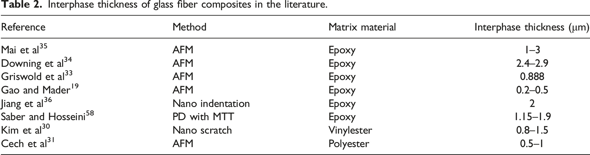
calculated the interphase thickness from 0.5 to 1 μm and elastic modulus variation between 5 and 15 GPa for glass/polyester specimens. Researchers reported the interphase thickness for glass/epoxy composites between 20 nm and 3 μm utilizing the AFM test method.19,32–36 Some researchers also calculated the interphase elastic modulus as a profile between glass and epoxy.19,34 They also investigated the environmental effects on the interphase properties in FRP composites. Hodzic et al.
37
studied the interphase region in dry and water-aged polymer/glass composite materials with nanoindentation and scratch tests. Results showed the increase of interphase region width and degradation of the material properties during water aging. Also, using AFM tests, Riano et al.
38
showed that the interphase width increases up to 1 mm during aging in glass/epoxy composites.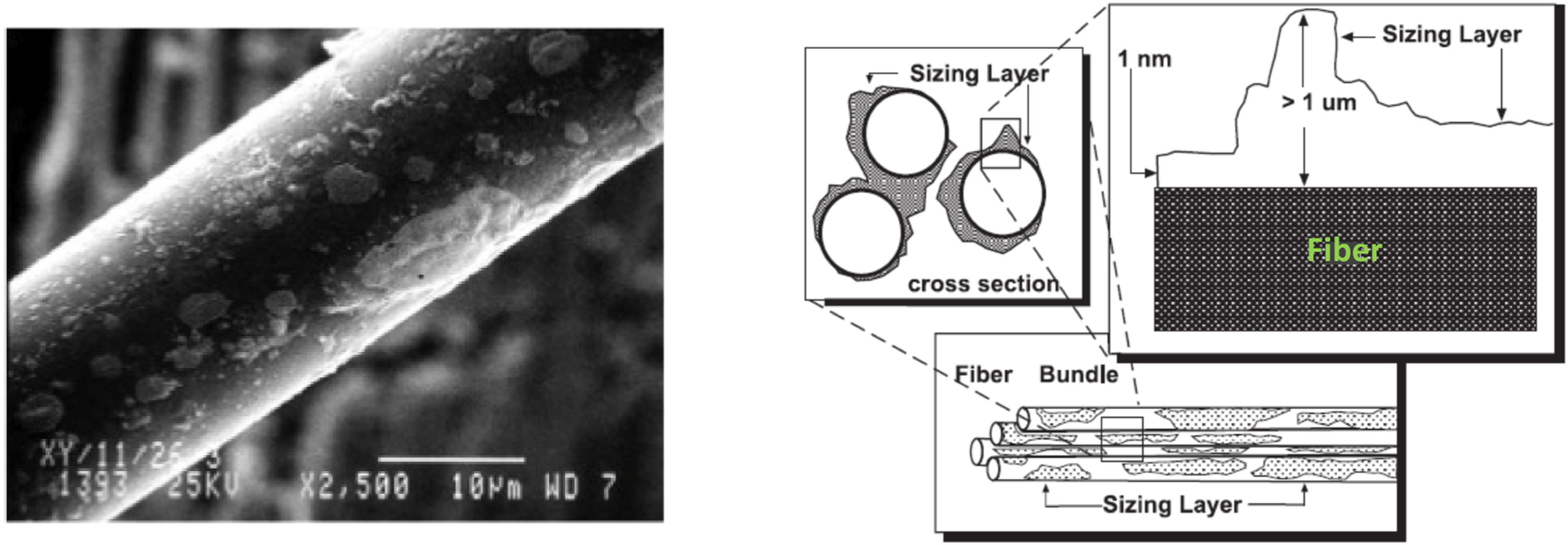
Peridynamic (PD) theory is a new non-local continuum mechanics formulation that was introduced by Silling 39 and Silling et al. 40 PD has great advantages over the classical continuum mechanics–based methods and molecular dynamic (MD) simulation methods. 41 In molecular dynamics (MD), the interaction distance between material particles is infinite, and every particle interacts with all particles in the bulk material. As a result, we restrict the time and length scale in the modelling and simulation in MD. In classical continuum mechanics, each material point interacts with its adjacent points and hence it is a local theory. The finite element method (FEM) is also a continuum method vastly employed in complex models. However, interphase scale and meshing are challenging in this method. In FEM, unlike the PD method, the neighboring elements restricted each other in size from the adjacent nodes. It is known that a highly distorted mesh result in large errors and constant remeshing are impractical. 40 In PD method, the mass points are geometrically independent and only interact with each other by pairwise force. Also, in PD, one mass point represents a discretized cell instead of four (2D) or eight (3D) nodes for each element in FEM. In addition to considering the non-local effects, these advantages enable PD to model regions with different scales rather than FEM. Because of the integro-differential form of equation in PD, instead of partial differential in continuum mechanics, most studies including discontinuity solved from PD.42–45 In References 45 and 46,44, 45 using the advantages of PD, damage in dual-phase (DP) material is predicted in the RVE that is extracted from the real microstructure. Ahmadi et al. 45 utilized the state-based PD and predicted the mechanical response, elastic-plastic deformation, and damage initiation and propagation in DP material. However, in a large model containing local cracks, applying the PD method, because of the family members for each mass point, is computationally expensive. In these problems, the number of mass points and their family must be minimized or PD must be coupled with another method such as FEM. 46
The review of past investigations reveals that interphase characterizing methods have several challenging issues. In the simulation methods, they mainly ignored the real conditions such as environmental effects, production quality, chemical reactions, and similar items, and they used simplified assumptions to model the interphase region. On the other hand, in nanoscale tests such as AFM and scratch tests, the interphase thickness and elastic modulus are restricted to a typical position along and around the fiber. However, obtaining the overall interphase properties is more logical for the structural analysis of composite material than using local properties.
This paper introduces a hybrid technique to characterize interphase regions in composite materials. At first, micro tensile tests (MTT) are performed for small specimens with and without a single fiber using a constructed tensile testing device. The digital image correlation (DIC) method is also utilized to measure the gauge length displacements and strains in micro specimens. Then, the peridynamics (PD) method is used as a non-local approach to characterize the interphase thickness and elastic modulus gradient along the interphase thickness. The developed PD software can simulate the interphase as a nanoscale region in a macro domain of glass/epoxy. The developed procedure enables us to characterize the elastic modulus variation of interphase in composites. As an advantage, the obtained results from the developed procedure give the overall properties of interphase and are not limited to a specific location at the interphase area.
Peridynamic method and non-uniform discretization
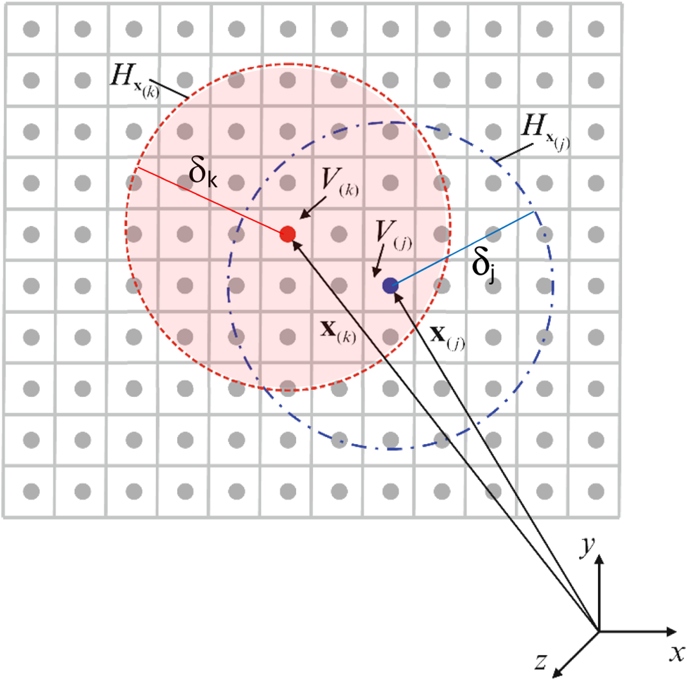
Peridynamic is a non-local theory that formulates problems in terms of integral equations rather than partial differential equations in classical mechanics. This method is a continuum model of molecular dynamics in which material particles interact across a finite distance called the horizon (δk). 47 All material particles (or material points in the discretized model) below the horizon distance constitute the family for every particle and are denoted by Hk.
Figure 2 shows the peridynamic parameters in a discretized domain. In this figure, Xk defines a mass point which is the representative of mass volumes of Vk. As explained, δk and Hk are horizon and family definitions in PD. Parameters in peridynamic.
48
In the ordinary state-based (OSB) peridynamic, the equation of motion for any particle of xk in the reference configuration is presented in (1). This equation is presented in a discretized form instead of an integral equation to be employed in numerical methods.

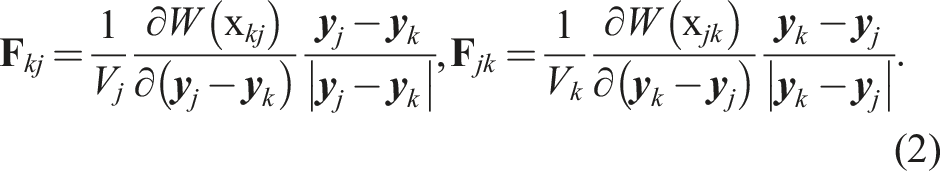
In which
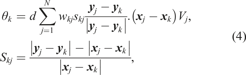
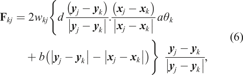
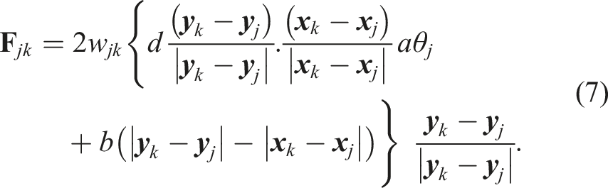
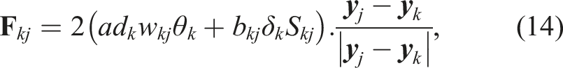
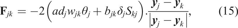
Therefore, by substituting the strain energy density in (2), the force density is extracted as below:
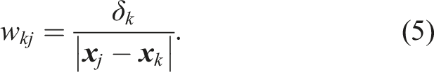
To calculate the PD constants, that is, a, b, and d, we compare the strain energy and dilatation in the PD method with classical continuum mechanics. In these methods, both the strain energy and dilatation are calculated due to isotropic expansion and simple shear loading:
48
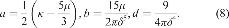
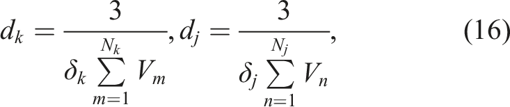
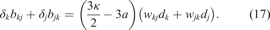
Because in composite materials, the bonding force between pairs of material points may pass through the different domains of material, it is necessary to modify the bulk modulus and shear modulus coefficients as follows:
49
The PD formulations were presented above belong to the regular discretization of material domain. However, a material domain with complex geometry may need to discretize with irregular or non-uniform patterns. In these cases, depending on the type of geometry and problem, it is necessary to use finer discretization in some locations. However, using fine and uniform discretization causes the increase of material points in the whole domain. As a result, the computational cost dramatically increases, and some problems arise due to programming language limitations.
In non-uniform discretization, unlike uniform patterns, the horizon is different for each material point. However, employing the variable horizon leads to the so-called ghost force effect. Figure 3(a) shows material points denoted by k and j indexes with different horizons. In this condition, point k may choose j as a family member, but point j may not candidate point k as a family member. This is the main reason for the ghost force. In which, material point k interacts with j, but j doesn’t have any interaction with k. Family points in non-uniform discretization (a), addition criteria (b), and deletion criteria (c).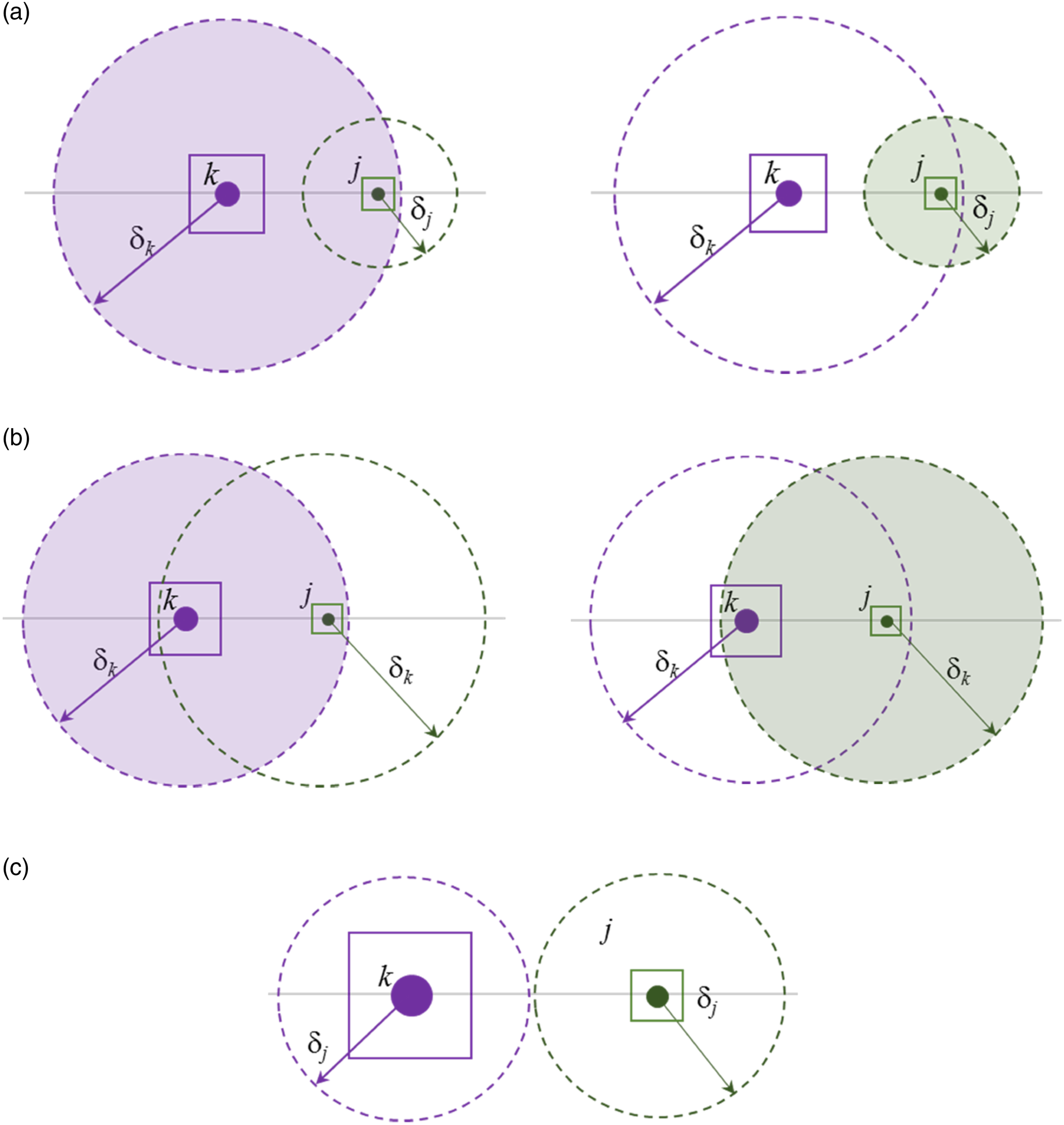
To prevent this difficulty, we should create family conditions so that if point j chooses point k, point k also chooses point j. 50 This method is known as the “addition criteria” in family creation. The other method is the “deletion criteria,” in which none of the j and k points select each other. As a result, if the larger horizon is assigned between two material points, we apply the “addition criteria”, and if we set the smaller horizon, we use the “deletion criteria.” These methods are shown in Figure 3(b) and (c).
In the peridynamic method, choosing the horizon size is also an important parameter. Investigations reveal that the best horizon size is 3D or greater, in which Family (green area) in addition (a) and deletion (b) criteria.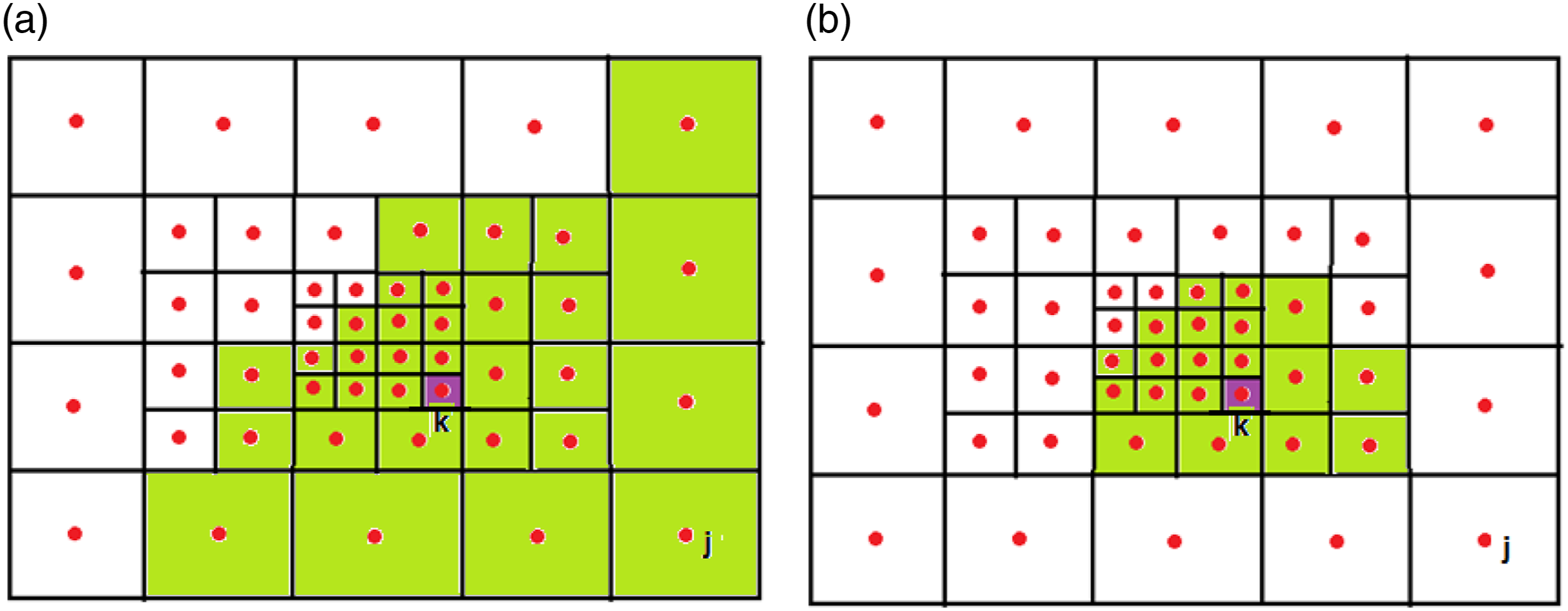
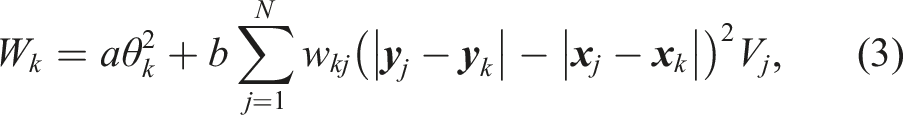
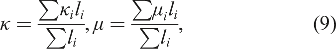
As mentioned before, for models with non-uniform discretization, the horizon size is varied at different points. Therefore, the contributions of material points, for example, k and j, in the strain energy of
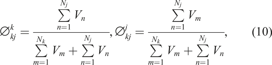
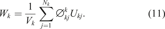
Considering the relation (3), the strain energy density in non-uniform discretization for isotropic material is rewritten as follows:
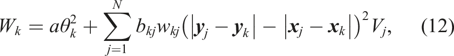
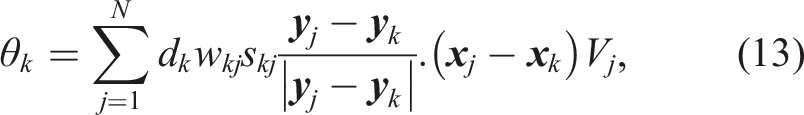
Consequently, the final form of the PD equation of motion is generated by substituting

This PD equation can be solved for static problems by using adaptive dynamic relaxation (ADR), 52 which modifies the dynamic relaxation technique. 53 An extension of this method for obtaining steady-state solutions of non-linear peridynamic equations has been presented in Ref. 54.
In the PD method, the stress vector can also be obtained from the following expression:
55
This stress tensor must be calculated from the reaction force acting on one side of the material point.
Peridynamic modeling of interphase
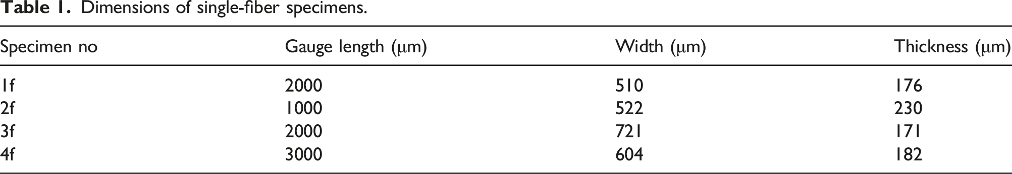
Dimensions of single-fiber specimens.
Interphase thickness of glass fiber composites in the literature.
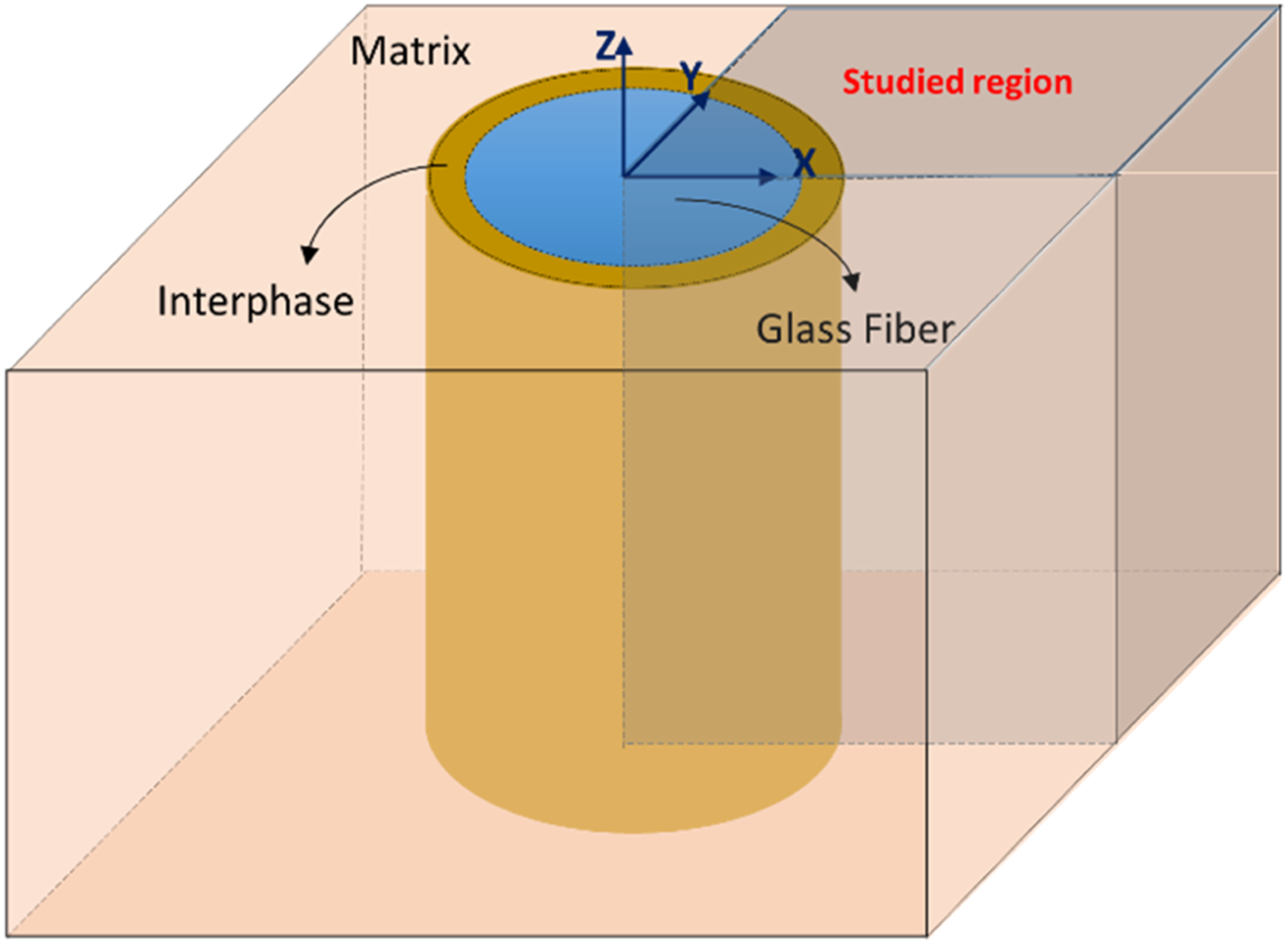
In peridynamic modelling, the material is divided into a series of material points, each of which represents a specific volume in the discretized material. The discretization size is an essential issue in extracting elastic modulus at the interphase region. Since the variation of elastic modulus near the fiber is exponential,19,30,36 the discretization up to 2 μm from the fiber must be refined enough. Figure 5 shows the compactness of material points at the interphase and the neighbor’s region. Material points in the Z direction (height) are also distributed with this resolution, and the material volumes are approximately cubic. To reduce the computational costs and due to the symmetry conditions, a quarter of the specimens are modelled (Figure 6). Peridynamic material points at quarter of specimen section (interphase, epoxy, and fiber). Illustration of different phases in single-fiber glass/epoxy specimen.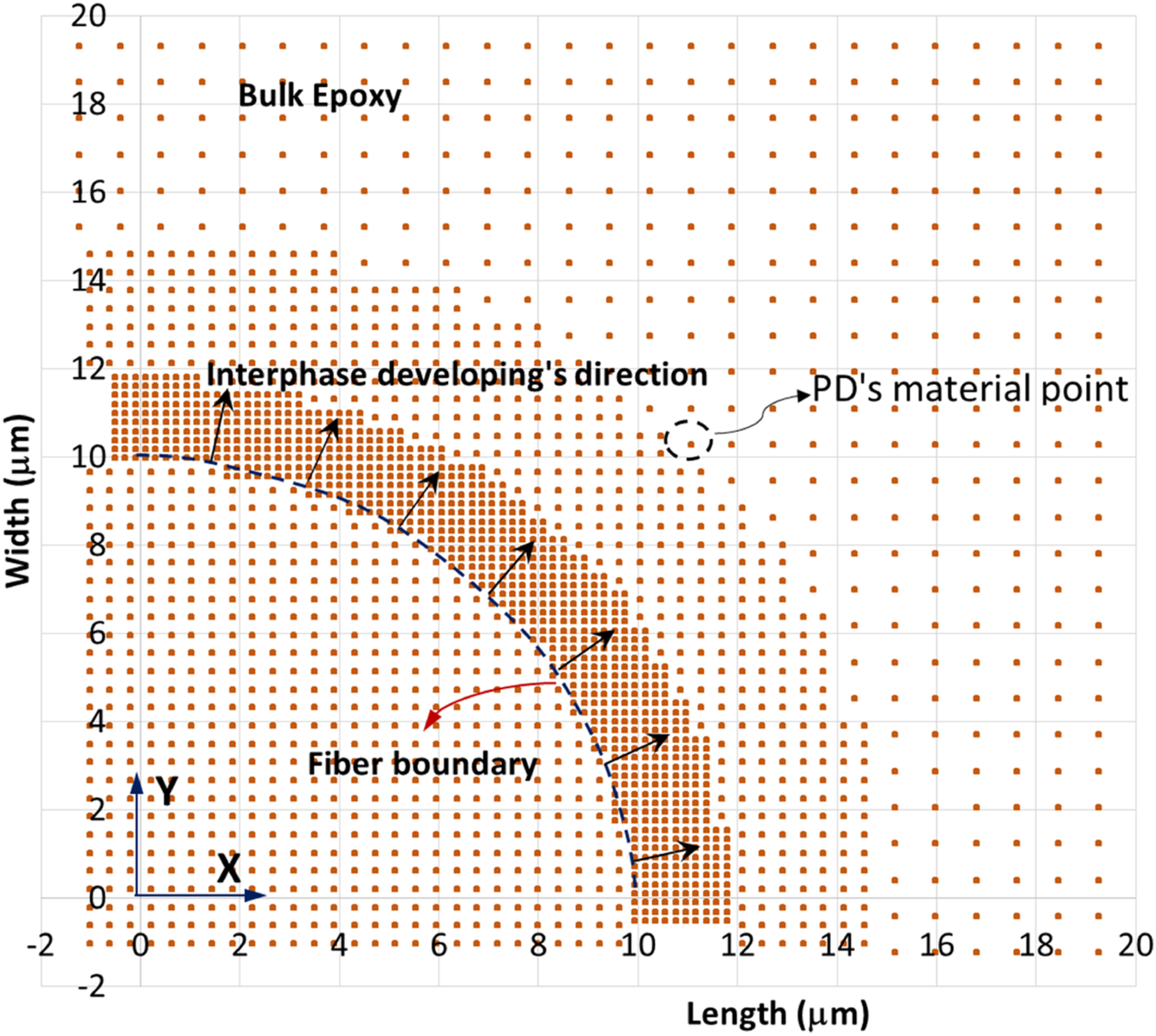
The family search process is one of the most time-consuming parts of a PD analysis. In the random search technique, all other points in the body are checked as family members for every material point. That means if the body has n material points, the number of family searches is n2. This process is time-consuming, especially for a 3D model.
To avoid too much time consumption during family creation, we use the partitioning technique. This technique divides the body into partitions, each of which contains some material points. Then, partition families are created for every partition by defining the proper horizon. Therefore, every material point searches between points in its partition family only. For example, as shown in Figure 7 the material point 1 searches between points in partitions of 2, 6, and 5 only instead of all points in the body. Typical model of partitioning in PD.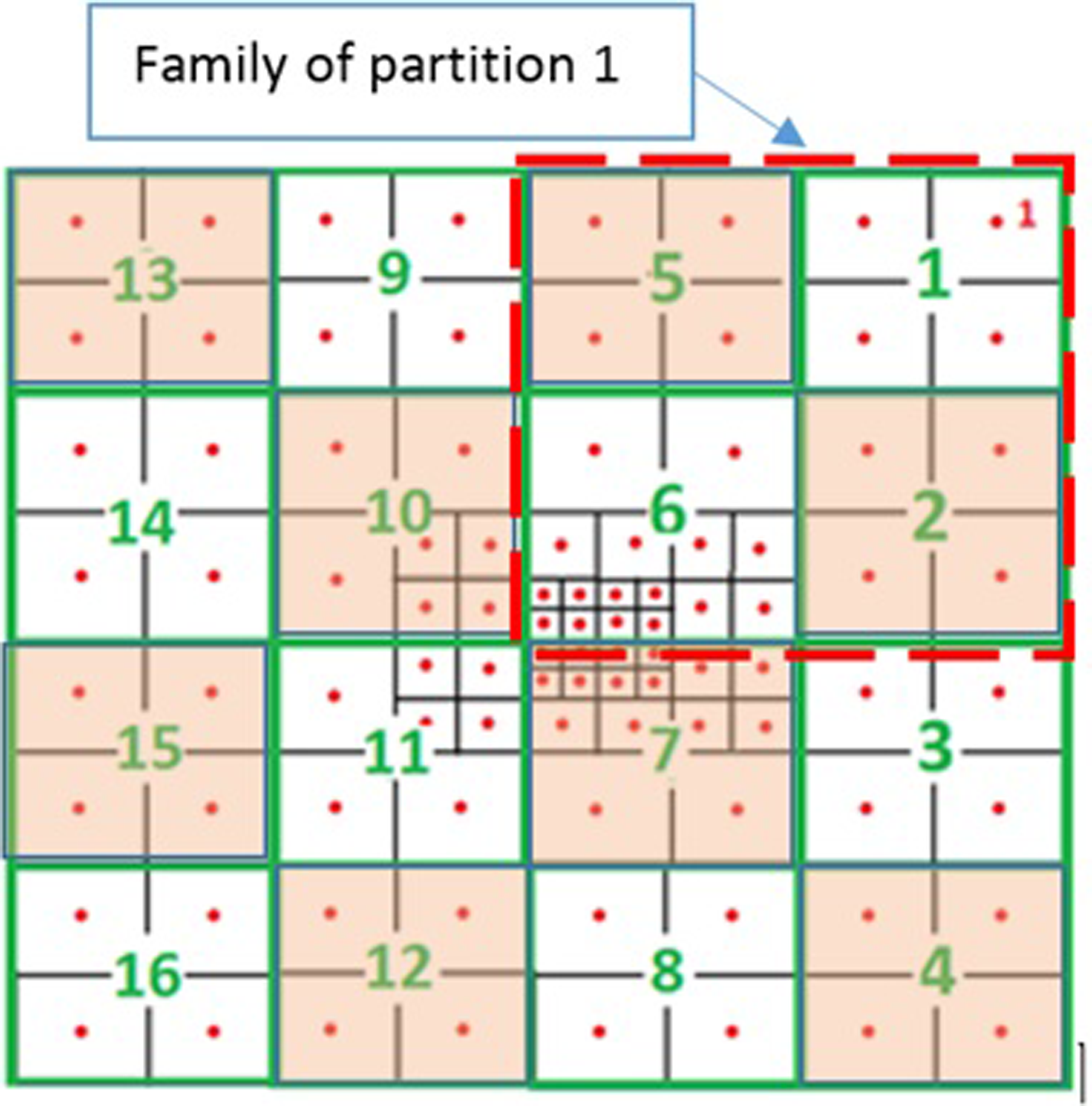
In these analyses, the elastic modulus of the fiber is 71 GPa, and the Poisson’s ratios for the epoxy, interphase, and glass fiber are 0.35, 0.3, and 0.23, respectively.19,56,57 Also, the elastic modulus of epoxy was calculated in the author’s previous work 58 and presented in the following section.
Micro tensile tests
Due to the micro-scale of the interphase region, the single-glass fiber/epoxy specimens should be as small as possible. Therefore, a particular micro tensile testing device was constructed because of the specimen size. Also, we need a proper technique for processing the obtained results. For this purpose, the image processing of the micro tensile tests was performed to measure the displacements and strains of the specimens.
Tensile test device
The manufactured small testing machine is shown in Figure 8. The machine is adjusted in the level position by the levelling sensor and screws to prevent side forces on the specimen. The loading mass was weighted with an accurate scale of 0.0001 g. The amount of force caused by this weight is equal to 1.6717 N. The specimens were located between the upper and lower grippers as shown in Figure 8(a). Micro tensile test setup. Test stand (a) and data recording system (b).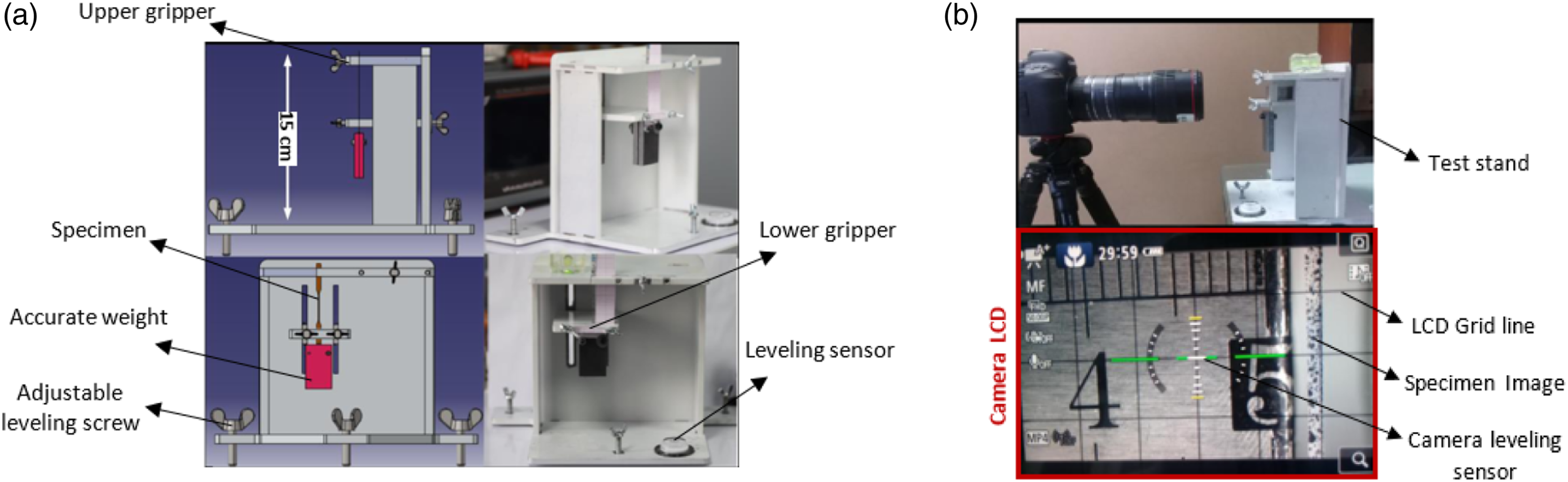
Data recording in micro tensile tests was performed by an optical method. For this purpose, a Canon EOS 6D Mark II camera was used. This camera takes images from the specimen during loading and unloading with a resolution of 50 frames per second. As shown in Figure 8(b), we can also level the camera by the levelling sensor and adjusting the tripod. These levelling instruments are essential and guarantee the camera is perpendicular to the specimen surface.
Specimen preparations
Making a single-fiber specimen is an affecting issue in the test results. Due to the micron size of the interphase, the specimens should be made as small as possible. To make these tinny specimens, we utilized silicone sheets with a thickness of 2 mm as molds. The molds were constructed by laser cutting inside a silicon sheet in the form of a dog bone. Also, two holes (0.2 mm in diameter) were created at the top and bottom of the molds on the asymmetric line to place the fiber correctly. After placing the fiber properly, the second silicon mold was put on the fiber. In this step, the mixed epoxy/hardener resin was injected into the mold. The specimen was kept at room temperature for several days to be cured. An epoxy specimen with similar dimensions was also made simultaneously for each single-fiber specimen to characterize epoxy elastic modulus.
By careful sanding, the size of the specimens was reduced as much as possible. During this process, the specimen’s dimensions were accurately controlled by a micrometer device. Table 1 shows the final dimensions of the single-fiber specimens.
After making the specimens, a pattern of color spots was created by spraying paint on each specimen. This pattern was required for DIC analyses in optical measurements. Figure 9 illustrates the created patterns on typical specimens. Color spot patterns on a typical specimen (a) and other specimens.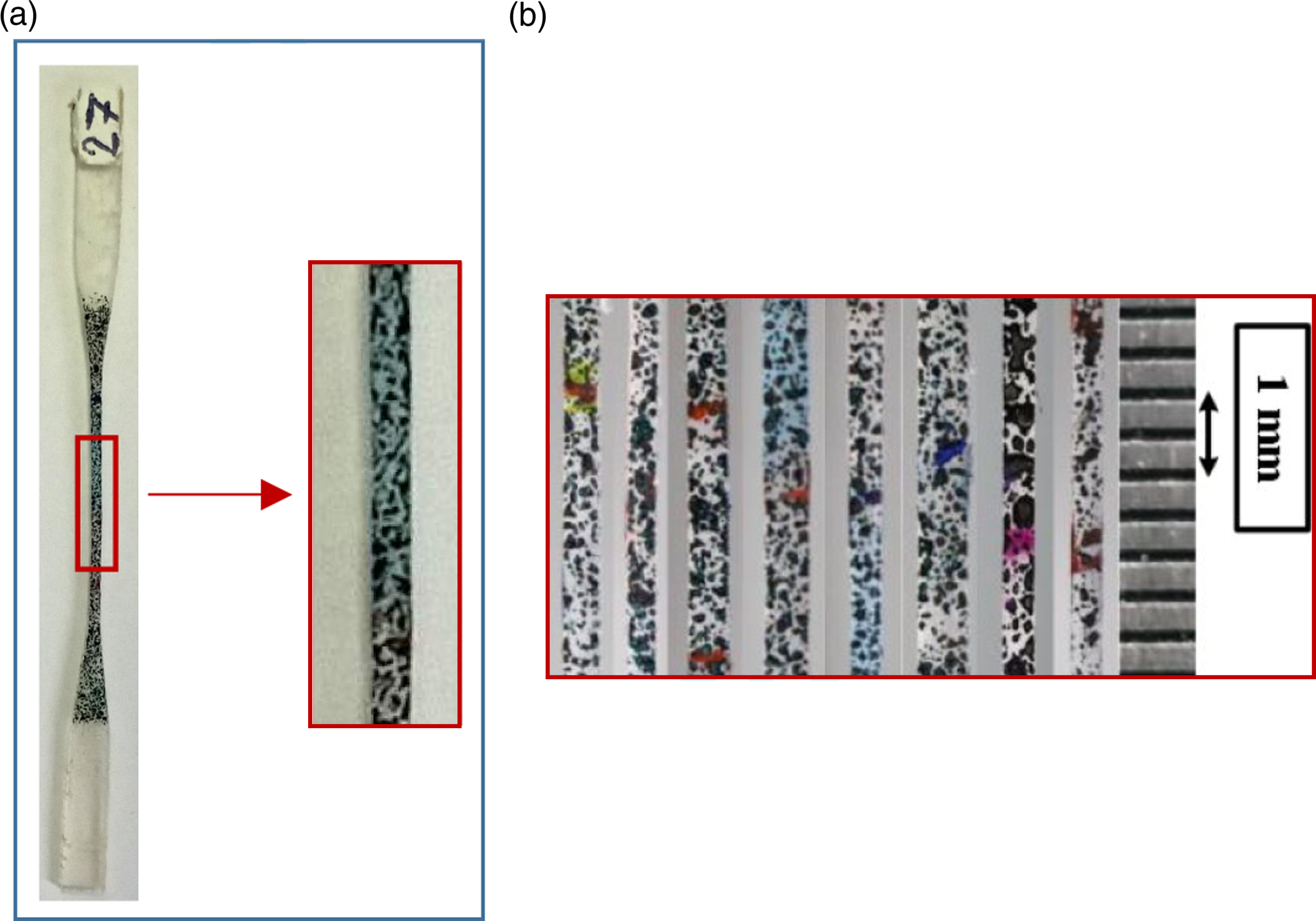
Tests results
We employed GOM 2016 software for image processing of optic video data extracted from micro tensile tests. In this procedure, software calibration takes place after entering the micro tensile test imaging into the software. In this step, the length scale is calibrated using a ruler next to the specimen (Figure 10(a)). Also, digital extensometers are placed on the gauge length for each specimen to track the displacements during the unloading. These digital extensometers are defined in the software. As far as the quality of the paint spot patterns is different for various specimens, the extensometer length may not be the same for all specimens. It is worth knowing that although the longer extensometer may reduce measurement errors, it increases the possibility of manufacturing defects and void in the measuring length. Image processing: (a) calibration and (b) extensometers assignment.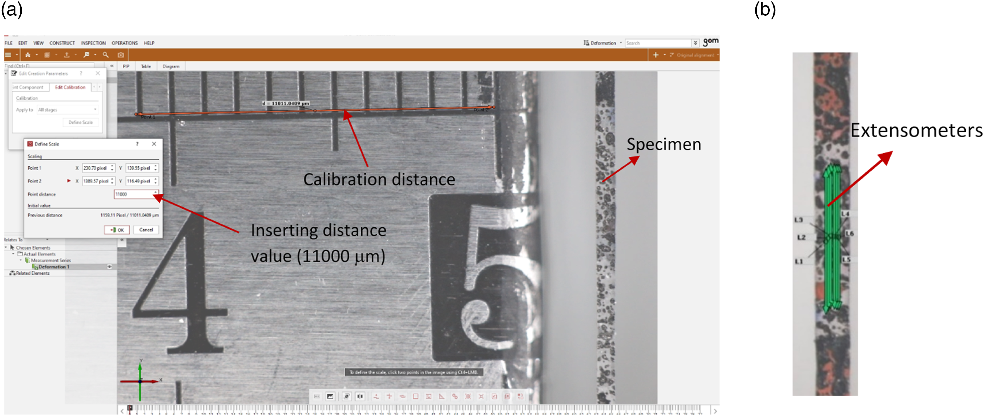
After defining the extensometer, we arrange extensometers at a distance of one pixel from each other along the specimen width and in the middle of specimen. In Figure 10(b), a typical arrangement of the digital extensometers as a software tool is illustrated. By magnifying the image in the DIC software, the image pixels are revealed. We used these pixels as a checkered plan to adjust the extensometer next to each other. This arrangement enables us to predict the strain variation across the specimen’s width and near the fiber/matrix interface.
We also performed several tensile tests for micro specimens of epoxy before single-fiber epoxy specimen tests (Figure 11). Based on the obtained results and performing peridynamic analyses for these specimens, the value of epoxy elastic modulus was between 2.88 and 3.09 GPa. These results are applied in the interphase characterization of single-fiber specimens. The authors also performed standard macro tensile tests based on the ASTM D638-14 for epoxy specimens and calculated the epoxy elastic modulus between 2.76 and 3.15 GPa. Comparison between the obtained results from the standard tests and micro tensile tests shows the accuracy of the measurements and computational procedure of the micro tensile test method. Tensile test of epoxy micro specimens.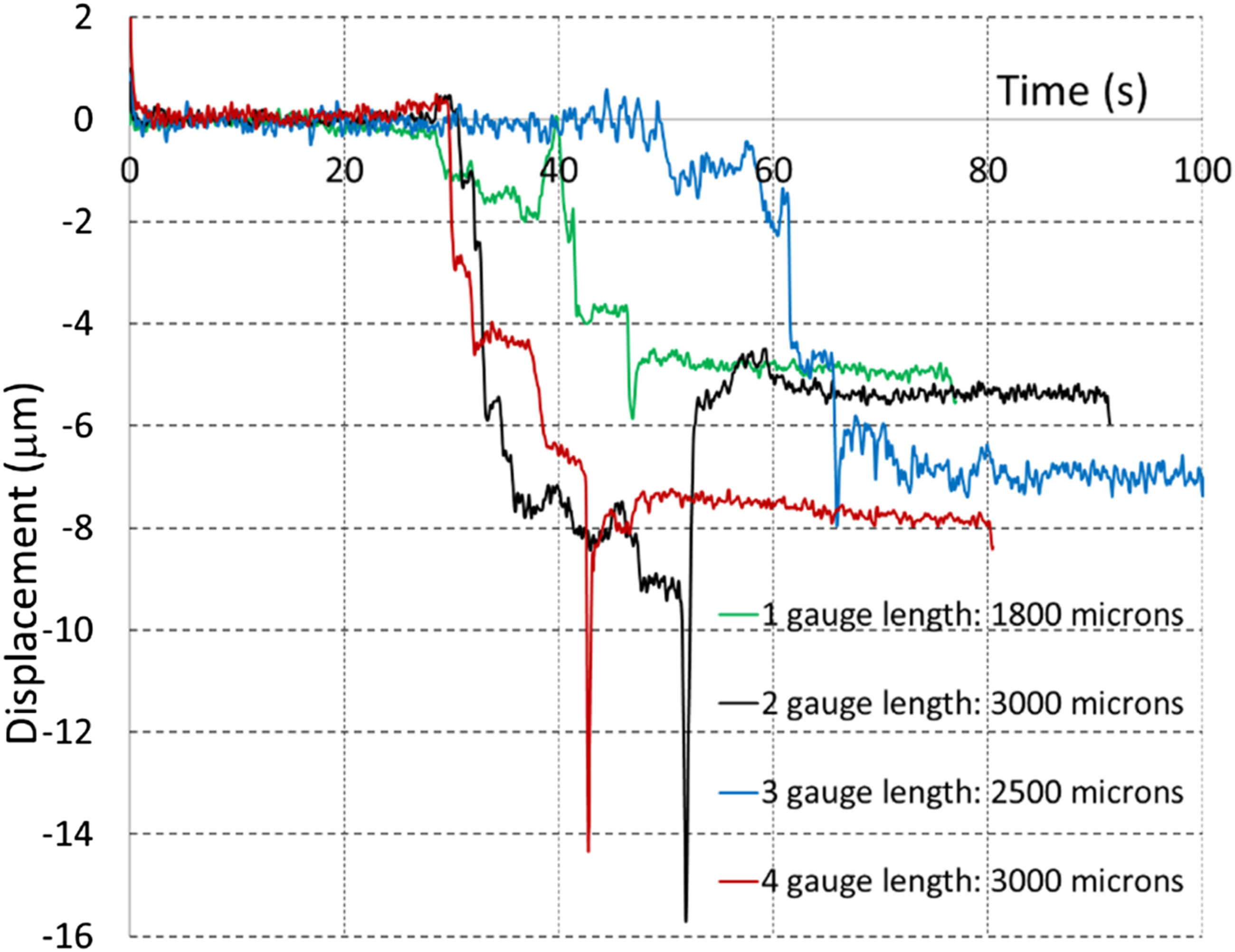
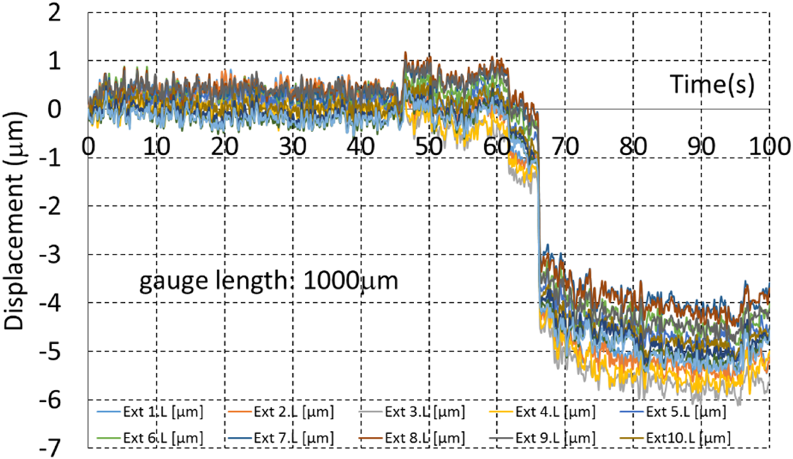
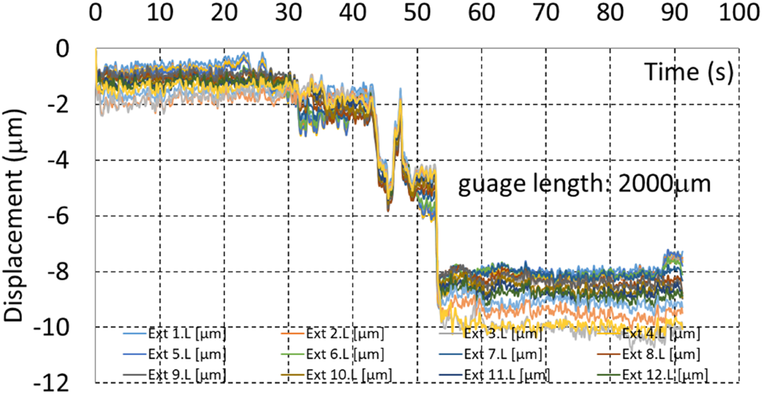
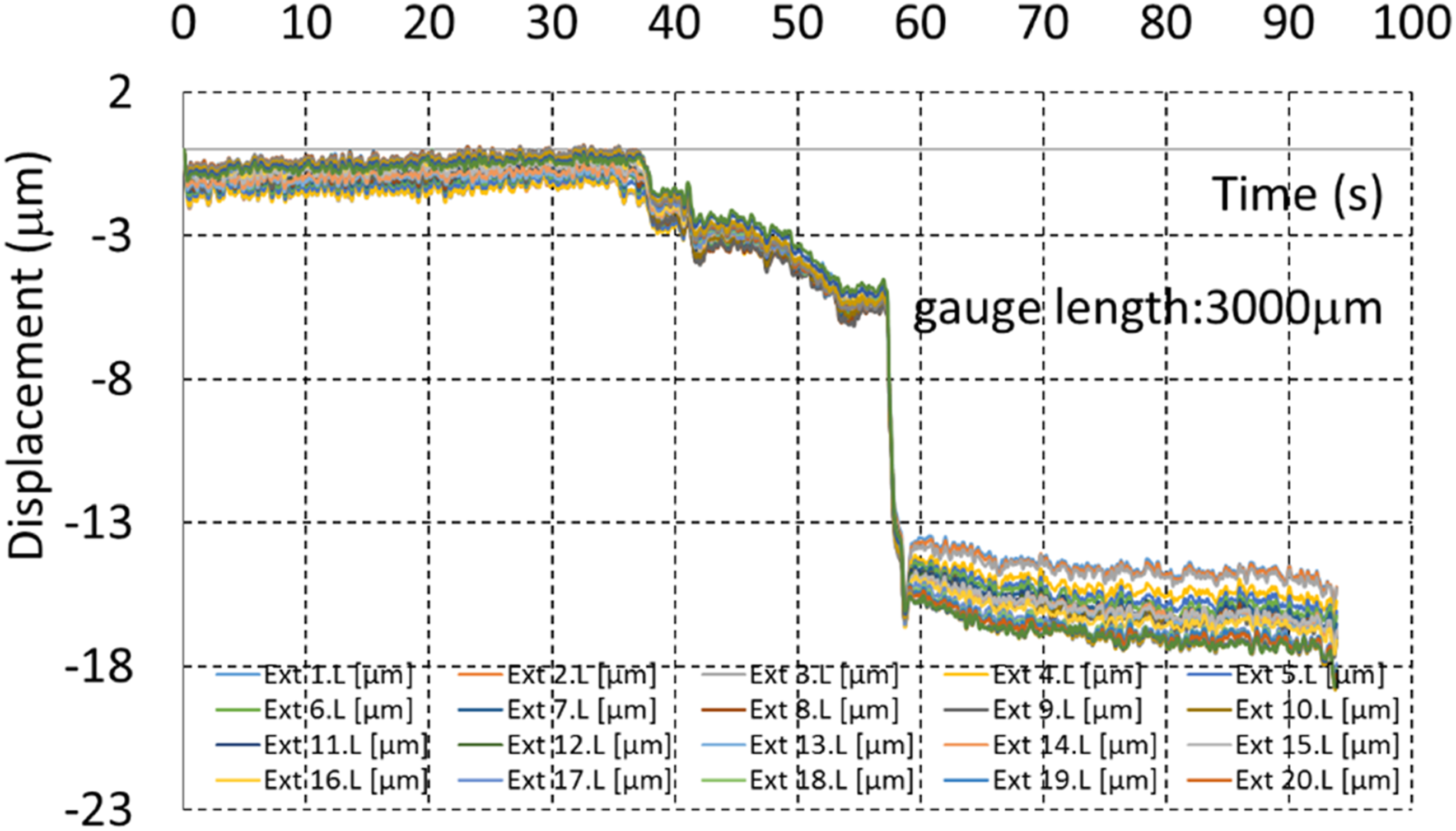
For the single-fiber specimen tests, the specimen was tied to the tensile testing machine from the top and then subjected to loading weight. After fixing the specimen from the bottom side, imaging started, and a few seconds later, the weight was released, and we waited to settle the specimen. The recorded imaging of the tensile test was entered into the image processing software, and the calibration and extensometer adjustments were performed. Figures 12–15 show the obtained displacements for different specimens. The maximum noise level of the displacement field is calculated at approximately 0.5 μm for all specimens. In the test results, we used the binomial filter to reduce the high noise level. Also to calculate the gauge displacements, we average data in 10 s–15 s (depending on the quality of graph) from the first part (before load releasing) of the displacement graph for every extensometer and also in the second part (released loading part) as shown in the following figure. Gauge displacements of specimen 1f across the width. Gauge displacement of specimen 2f across the width. Gauge displacement of specimen 3f across the width. Gauge displacement of specimen 4f across the width.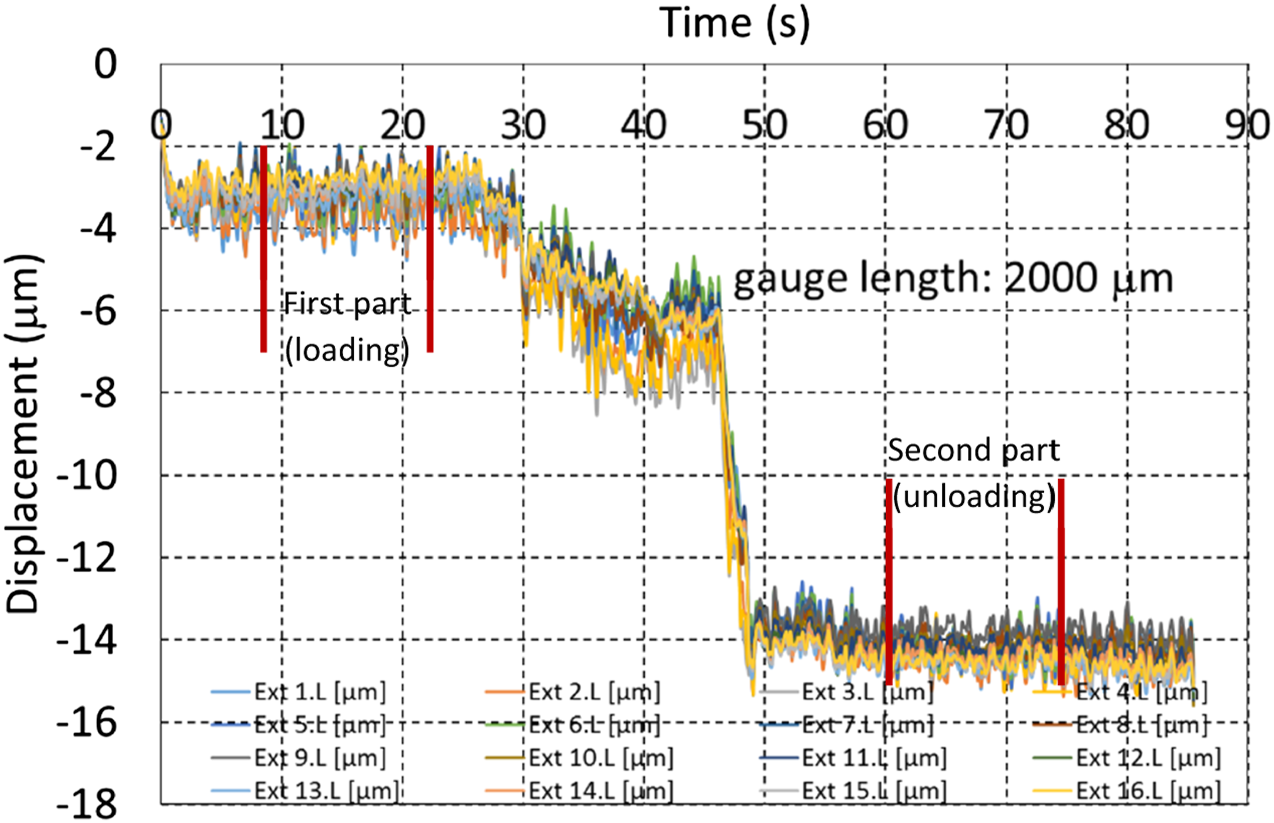
Results and discussions
Interphase material characterization
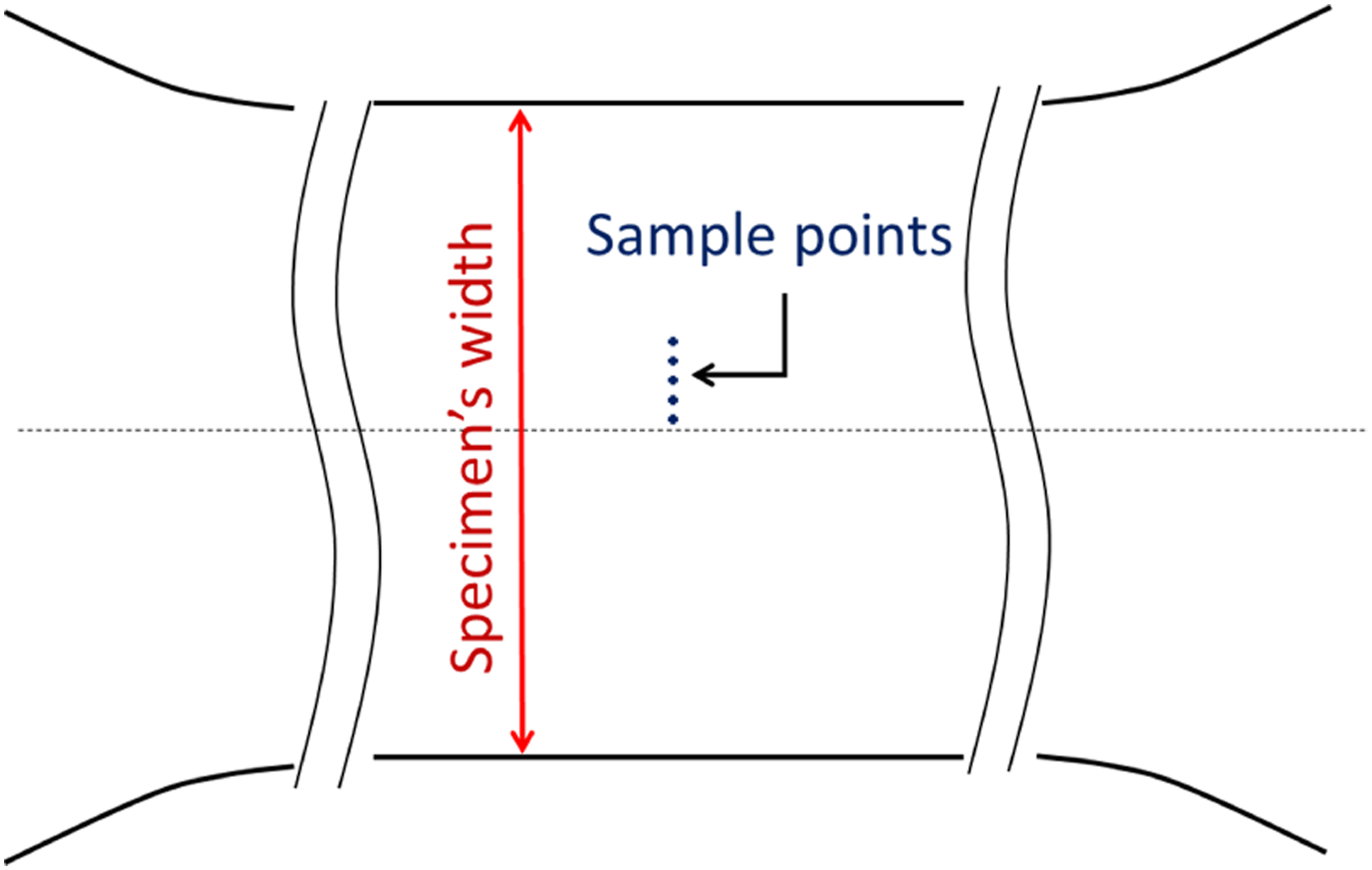
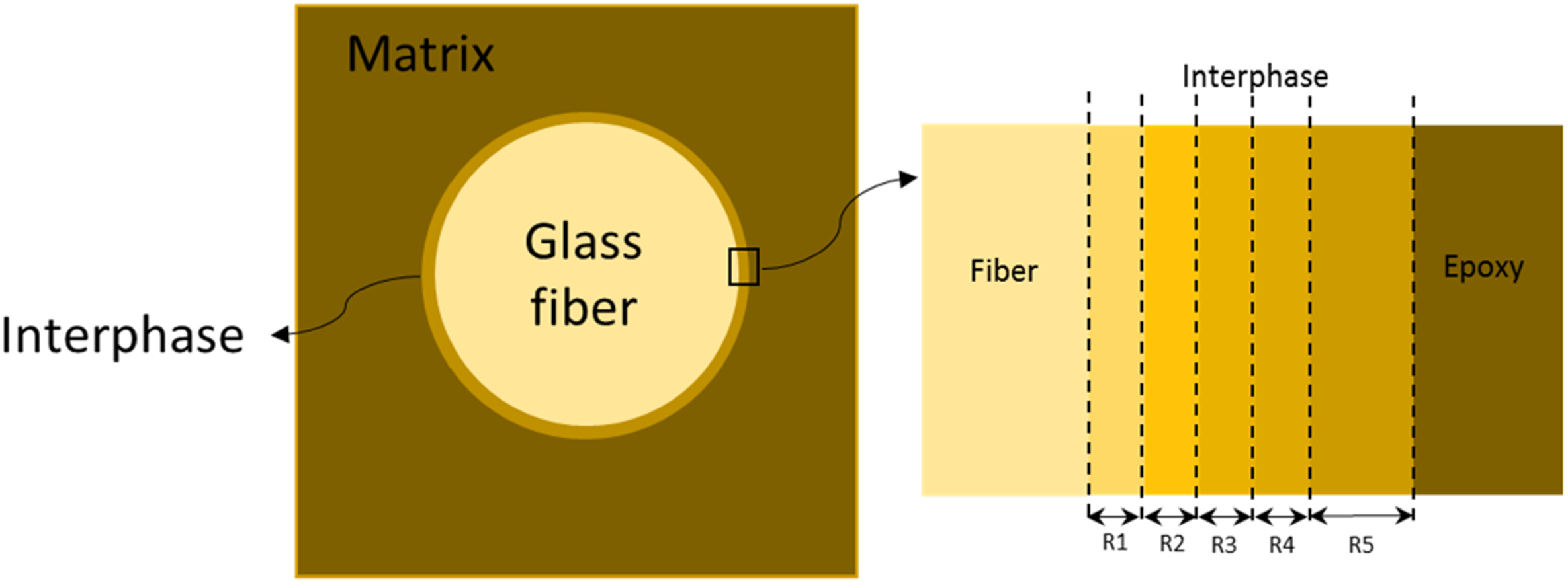
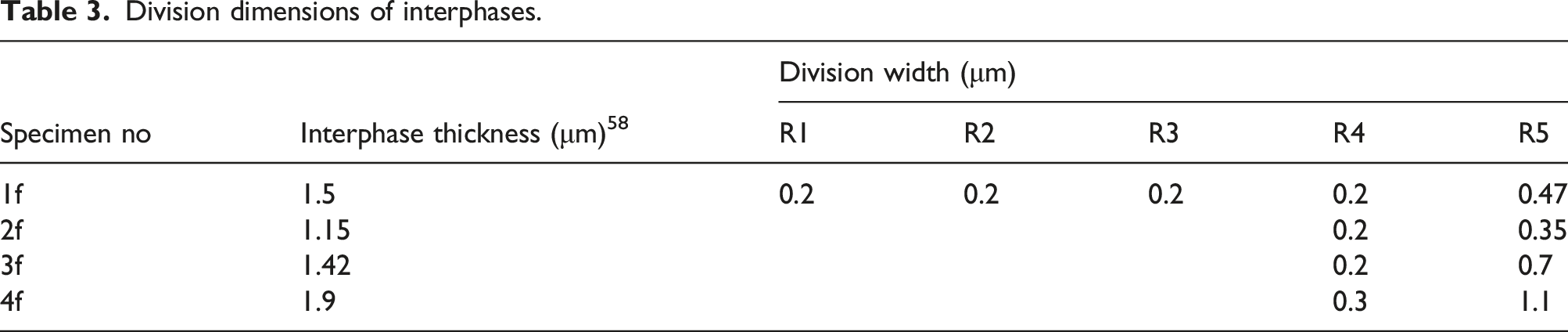
This paper aims to extract variations of elastic modulus along the thickness of the glass/epoxy interphase. Figure 16 shows the procedure of the interphase characterization. For this purpose, the single-fiber specimens under tension loading are modelled using the developed peridynamic software incorporated with an optimization technique to reach the same displacement variations across the specimens obtained from the DIC of experiments. These displacements were calculated in the previous section from the micro tensile tests. As shown in Figure 17, the target points are across the width and approximately 1.5 μm from each other. The interphase region was divided into five sections in PD code, and each division was assigned a different elastic modulus (Figure 18). The authors characterized the interphase thickness for every specimen in their previous work.
58
Based on these thicknesses, the width of each division for every interphase is presented in Table 3. Since the elastic modulus variation in the epoxy side of the interphase is small, a thicker division width was used in this region. Flowchart of interphase characterization. Target points near the fiber interface. Division of interphase region. Division dimensions of interphases.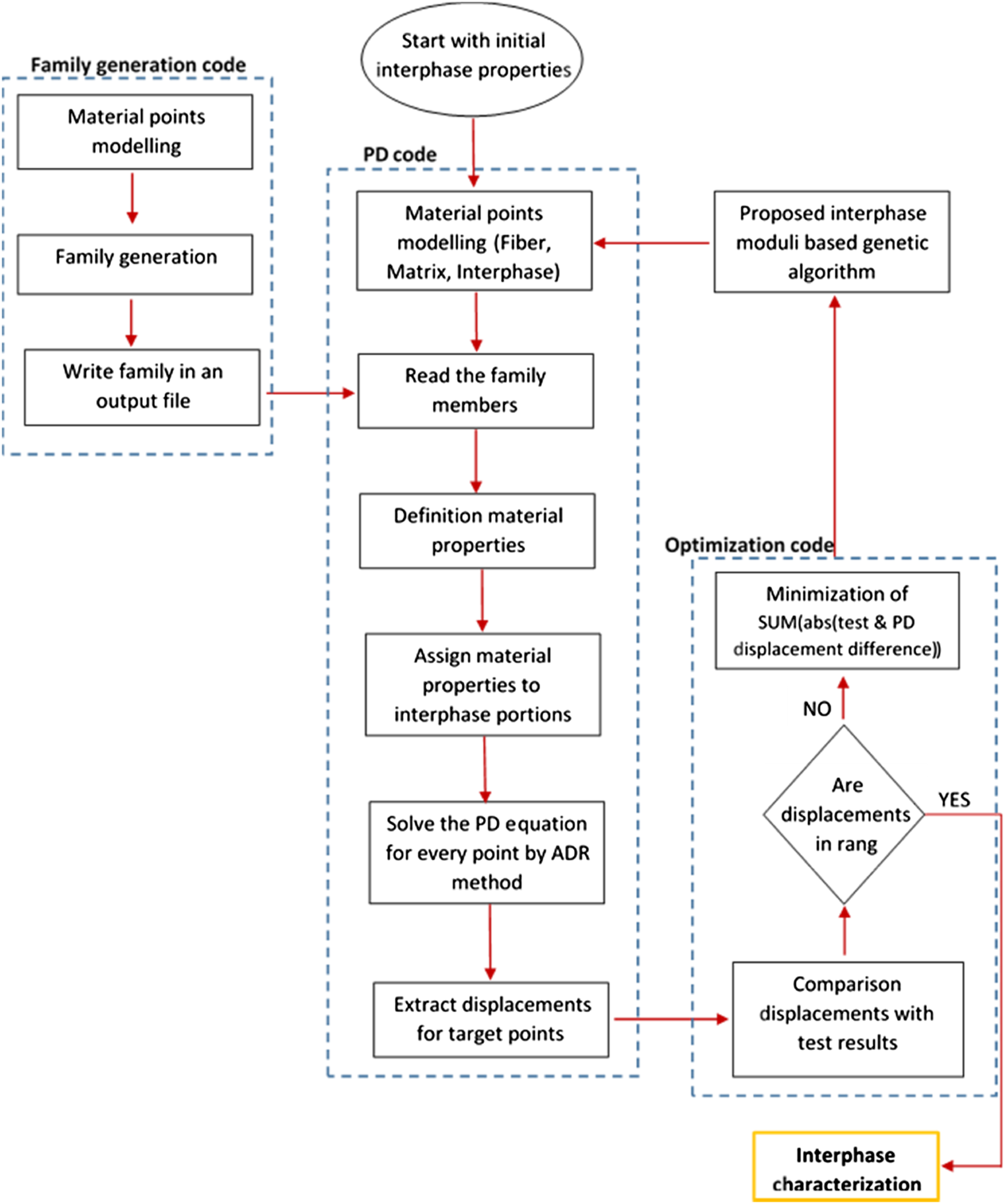
The peridynamic code is coupled with an optimization code that proposes the proper elastic moduli for the interphase sections. The obtained results from the optimization code are used in the developed PD software to solve the simulated specimens under tensile loading. In each step, the resulting displacements for the five points on the interphase are compared with the obtained values from the DIC of the experiments. This process continues to reach the best guess for elastic moduli. During interphase characterization, the optimization method should satisfy the following conditions:
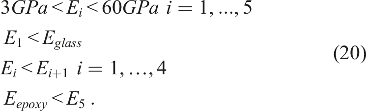
In which, Ei (i = 1, … , 5) is the elastic modulus for each division of the interphase. Also, an optimization function is defined for minimization as follows: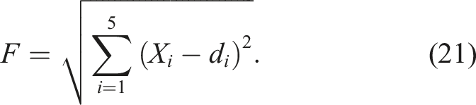
In this relation, Xi is the calculated displacement from the peridynamic code, and di is the experimental displacement value at each point. The following relation is also applied as a constraint:
By executing the coupled PD code and after some iterations, the elastic modulus profile for the interphase region is characterized.
Figures 19–22 show the obtained strains from peridynamic analyses after optimizing the elastic modulus for interphase divisions. These results are compared with the target values from the micro tensile test. Also, the distribution of strains is obtained for each specimen without considering any interphase region around the fiber interface. Strains of specimen 1f. Strains of specimen 2f. Strains of specimen 3f. Strains of specimen 4f.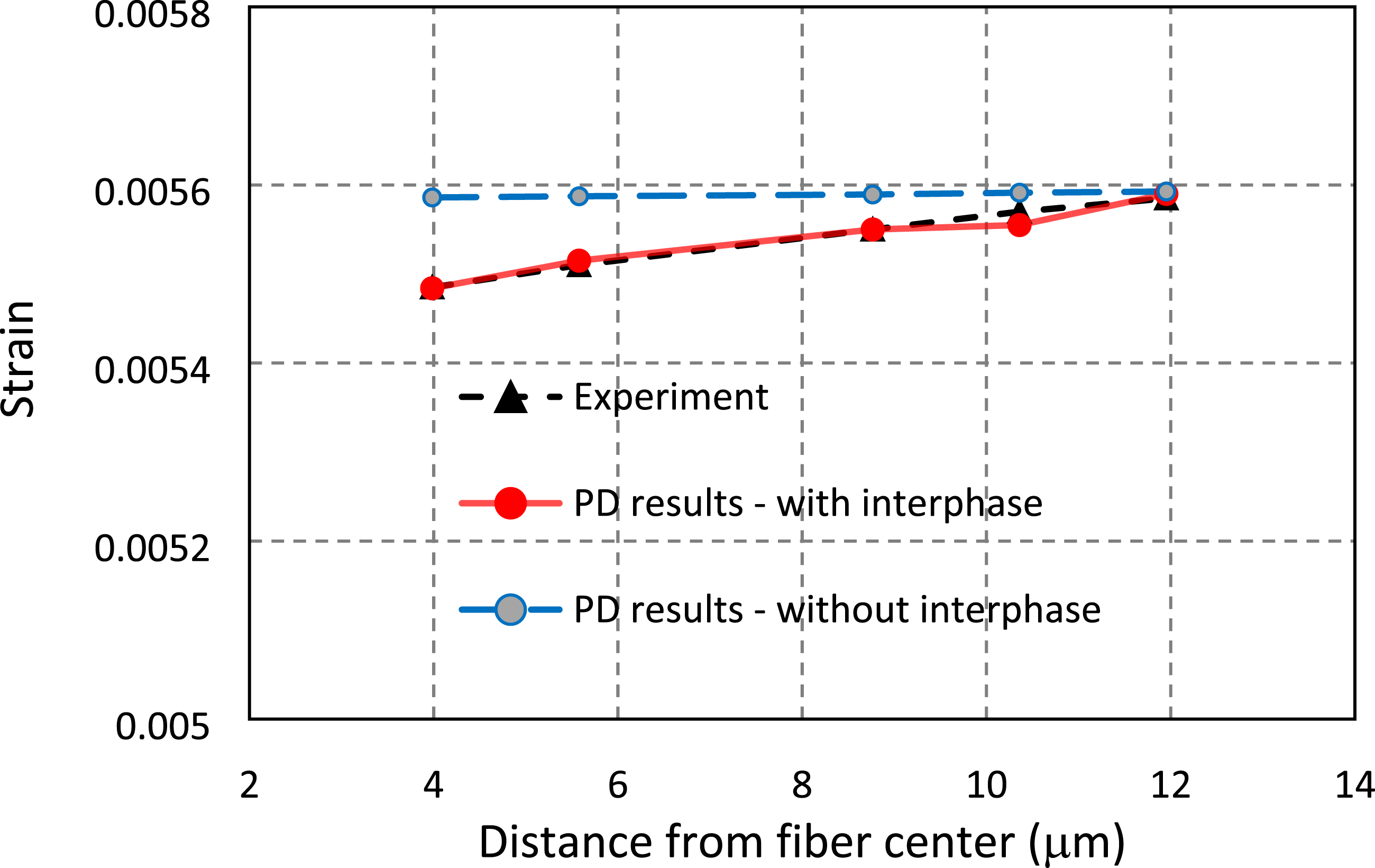
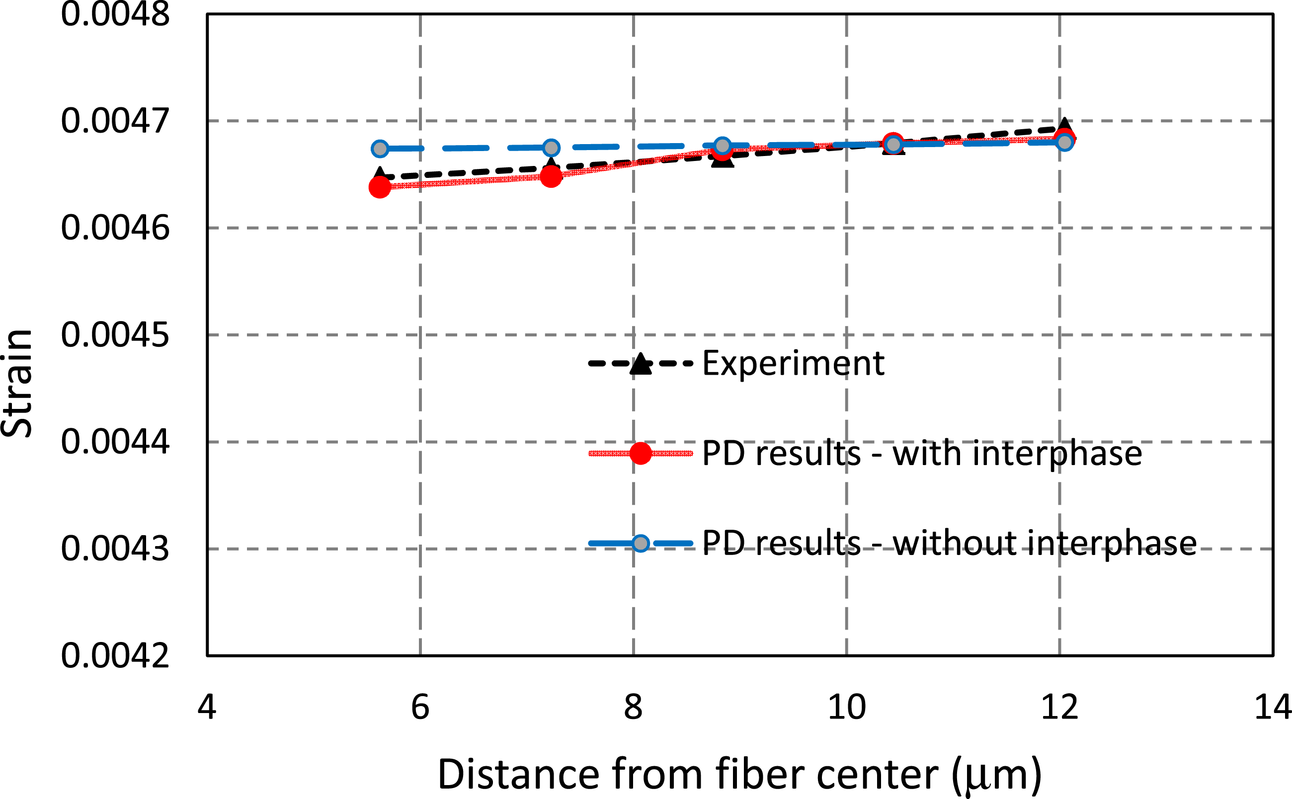
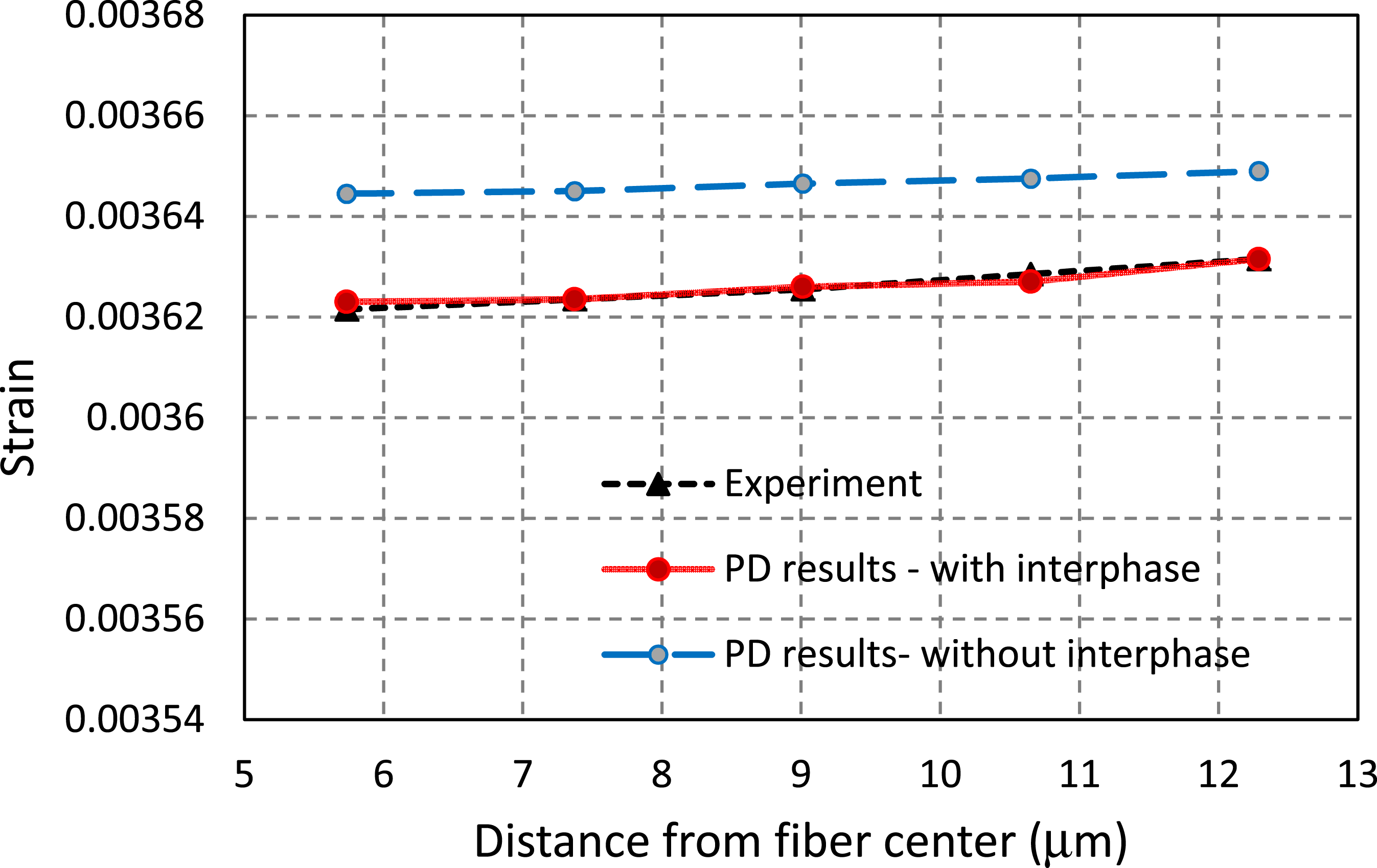
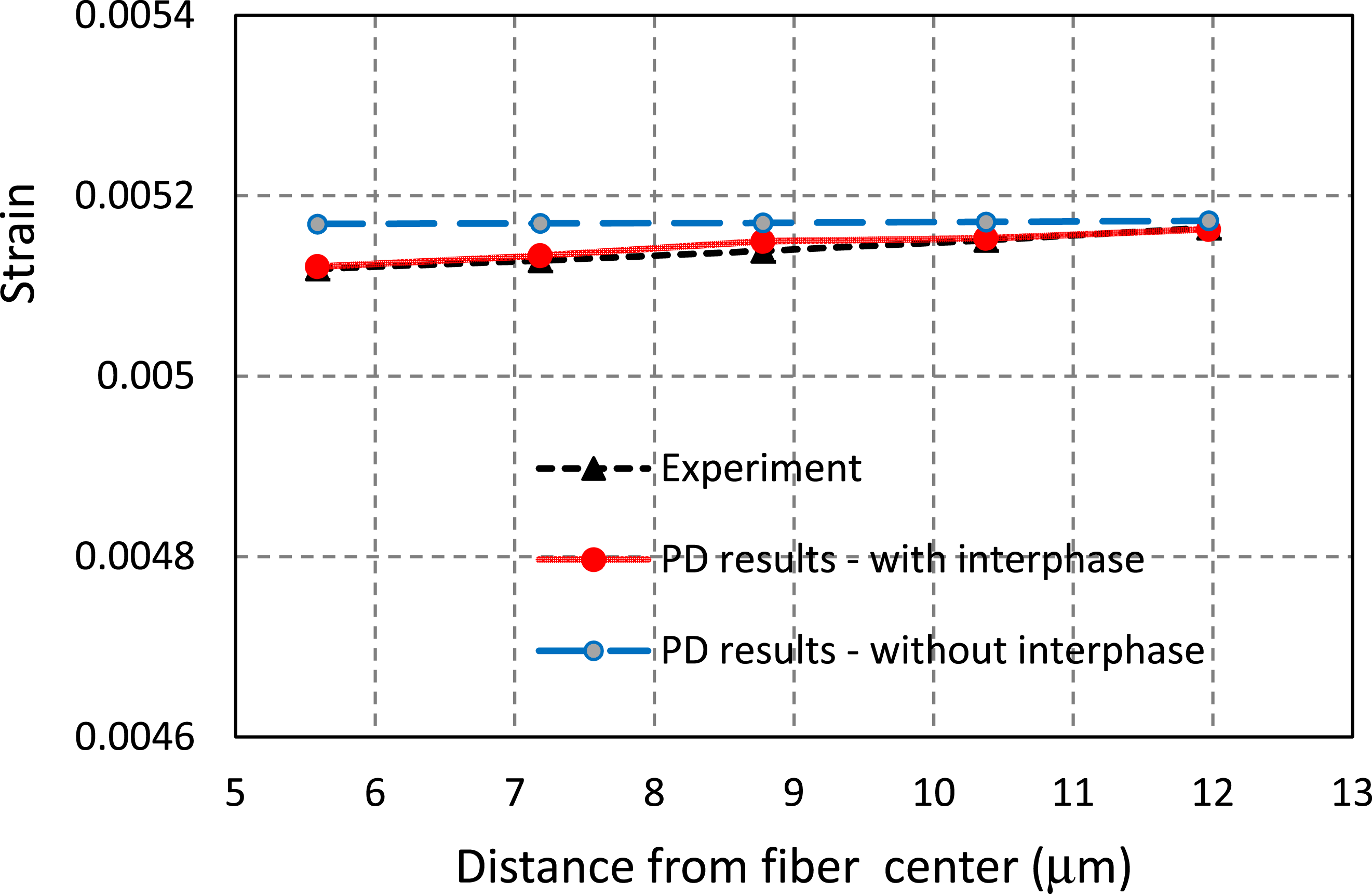
In all specimens, the obtained results from PD are in a good agreement with the experimental results. According to these results, the maximum deviation from the experimental values in specimens 1f, 2f, 3f, and 4f are 0.09%, 0.013%, 0.04%, and 0.41% respectively. Also, the graphs reveal that the existence of an interphase region can decrease the strain between 1e-4 and 2.2e-5 with respect to obtained results without the consideration of the interphase region.
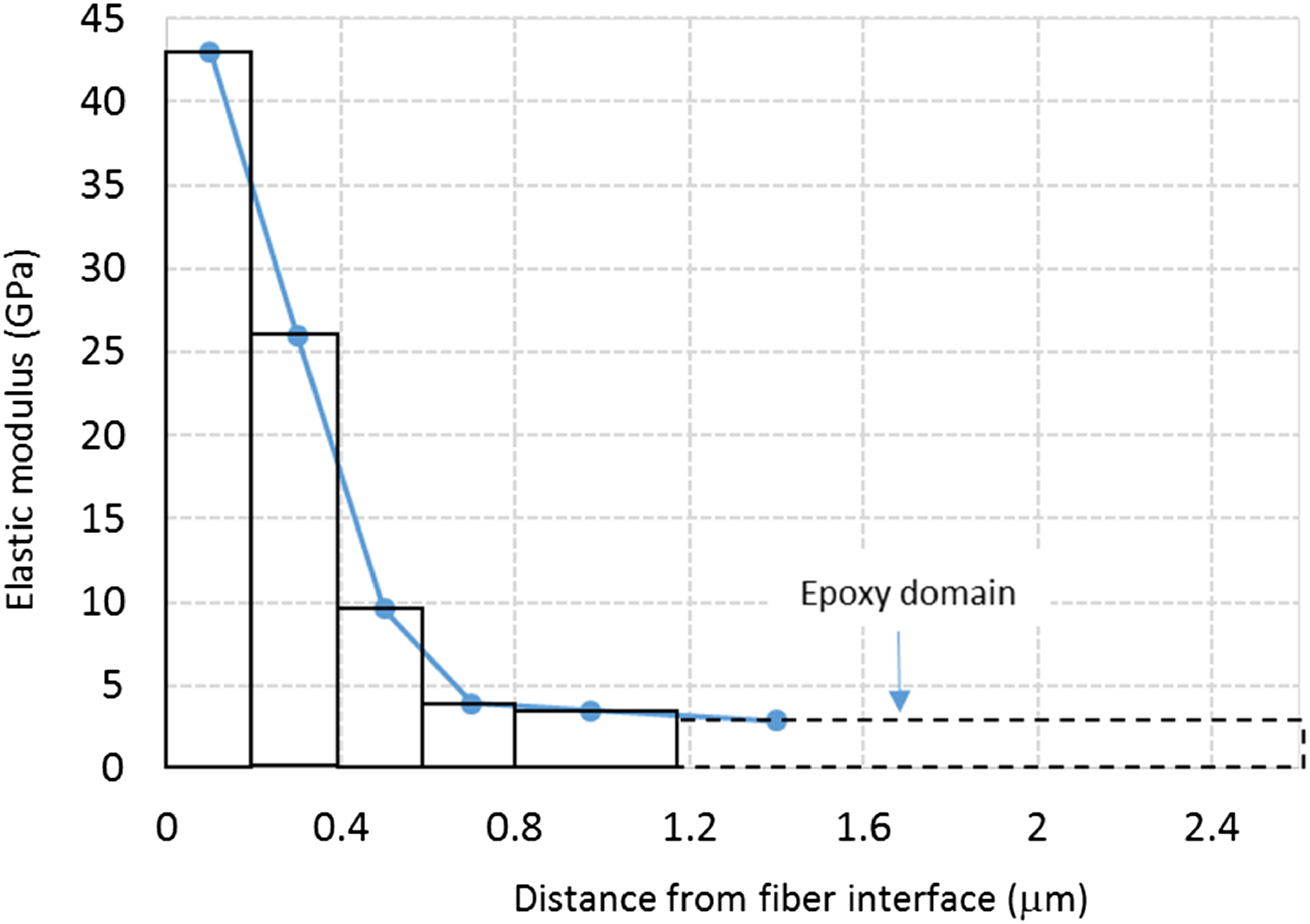
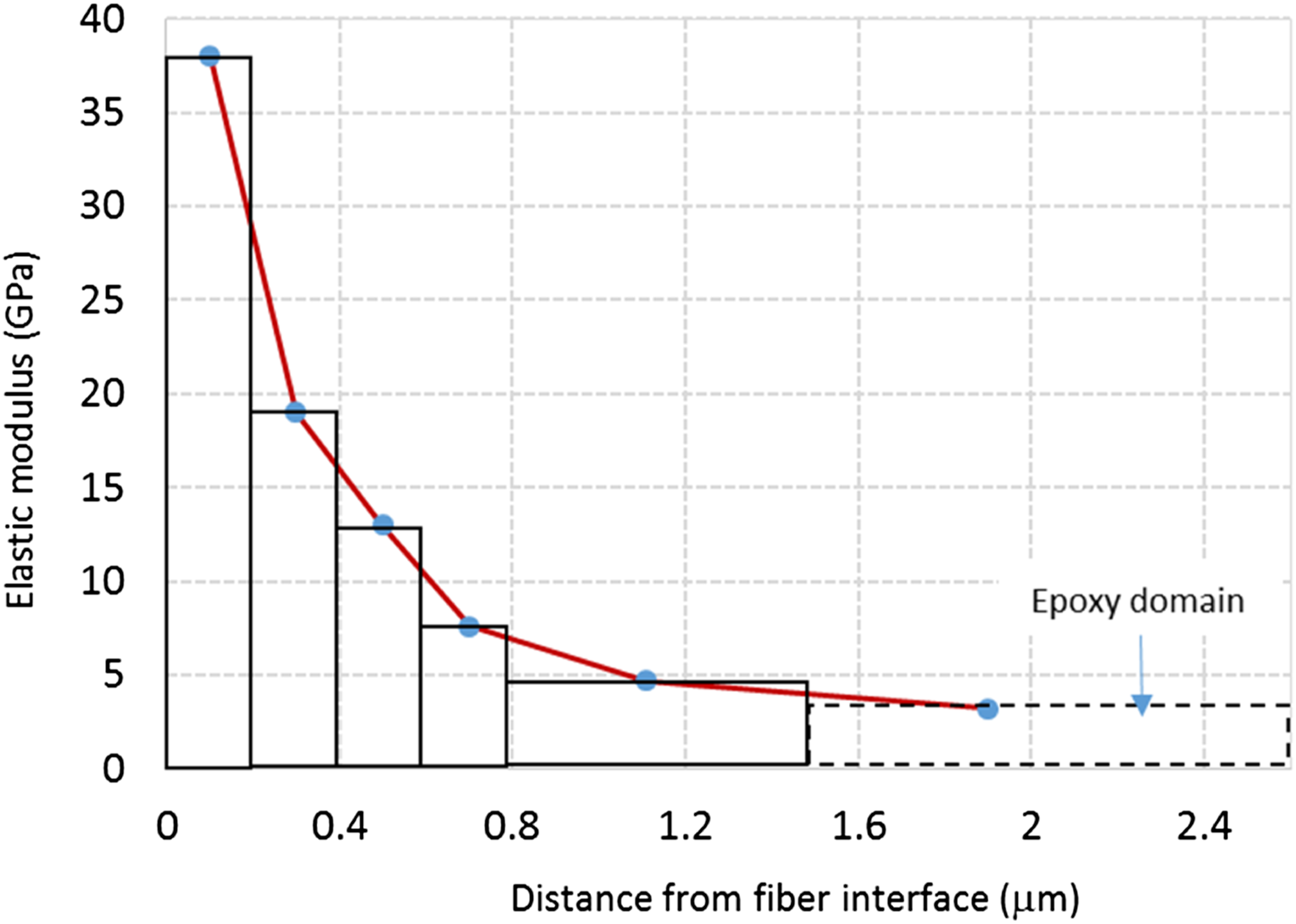
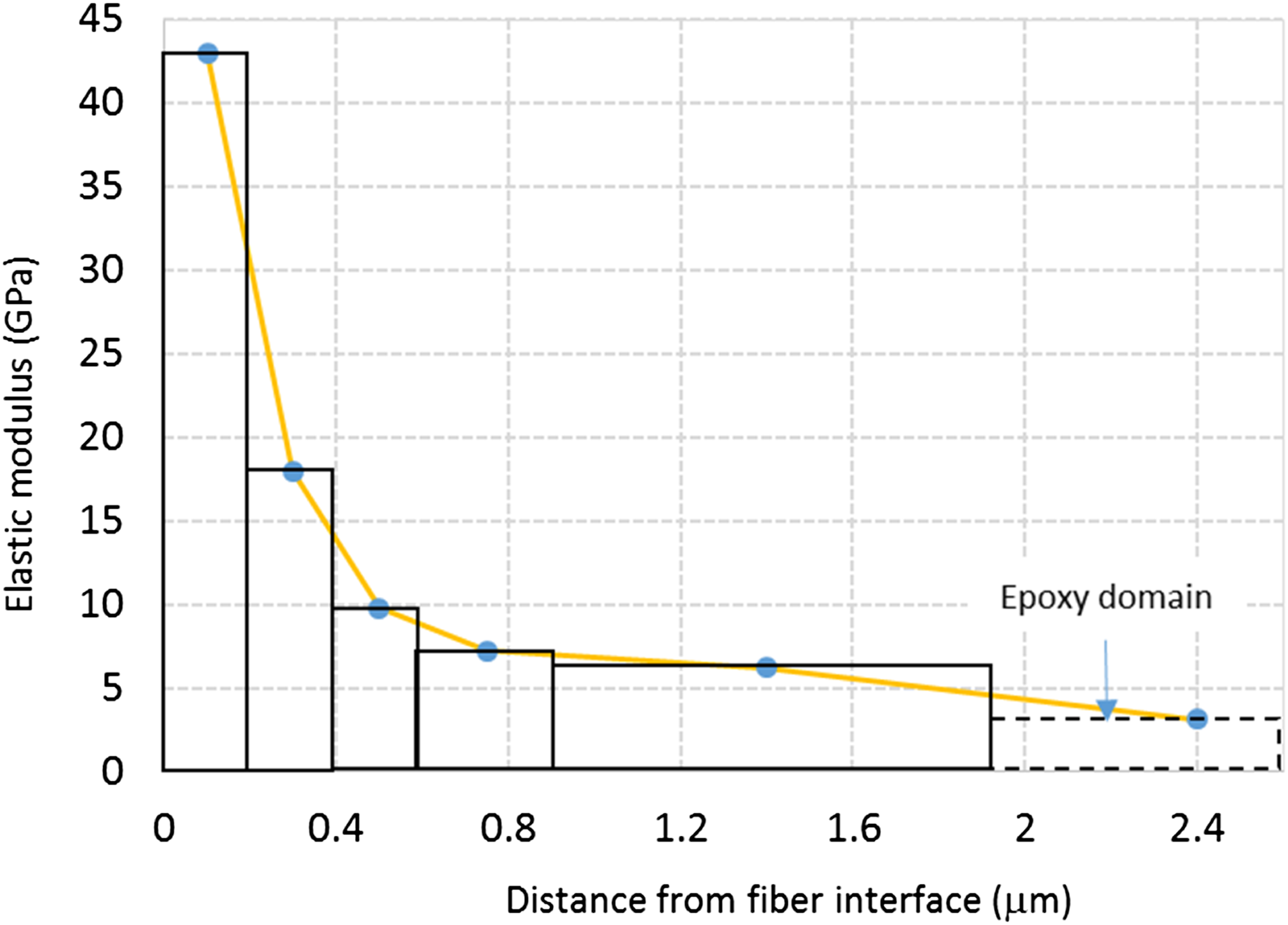
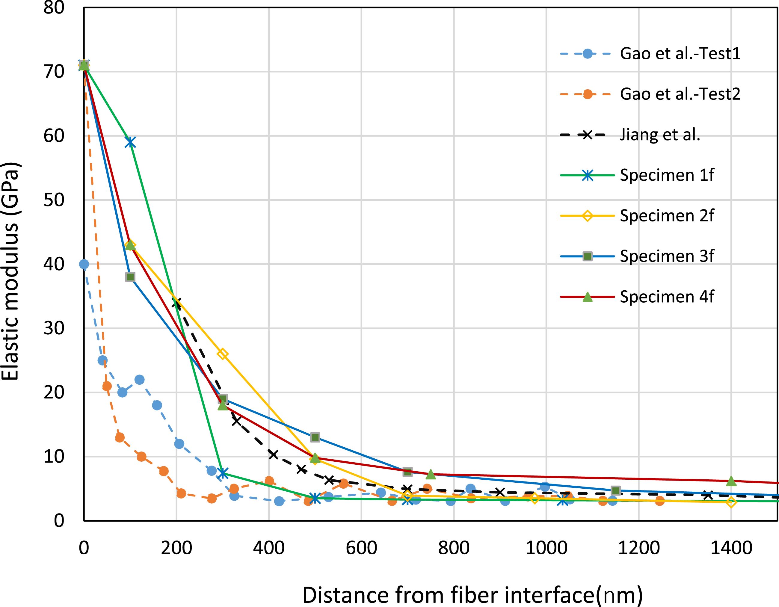
The previous strains were extracted from the calculated elastic moduli in the last stage of the PD analyses. The obtained variations of interphase elastic moduli are illustrated in Figures 23–26. All specimens show that the elastic modulus has the maximum value at the fiber’s interface and decreases with a steep slope to approach the epoxy elastic modulus. The maximum elastic modulus in the first section (adjacent to the fiber) of the interphase is about 40 (±3) GPa, except for specimen 1f (59 GPa), and it reaches to the epoxy modulus at a distance of 1.5 (±0.35) μm from fiber interface. The obtained results are compared with the available results of nano tests in the literature. Gao and Madar
19
obtained the variation of elastic modulus for the interphase region in glass/epoxy composites by the AFM test method. They used glass fiber with γ-APS silane coating. Recently, Jiang et al.
36
investigated the interphase properties of hybrid glass/carbon fiber in epoxy resin using the AFM method. They characterized elastic modulus variation of the glass/epoxy interphase in 2 μm thickness. The obtained results from the explained references are compared with those obtained in the current investigation in Figure 27. The results are in the correct range of the nano test presented in the literature. The little differences between the results come from the manufacturing process and the local interphase characterization in various investigations. Elastic modulus profile at the interphase of specimen 1f. Elastic modulus profile at the interphase of specimen 2f. Elastic modulus profile at the interphase of specimen 3f. Elastic modulus profile at the interphase of specimen 4f. Comparisons of the obtained variation of elastic modulus with those available in the literature.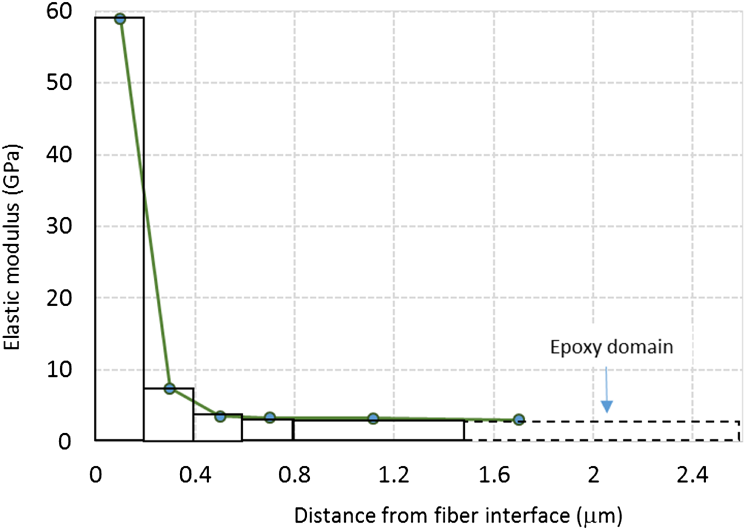
Stress and strain analyses
In this section, the obtained stresses and strains from peridynamic analyses of specimens considering different hypotheses for the interphase region, that is, variable elastic modulus, uniform elastic modulus, and without interphase region, are presented. For this purpose, we used the characterized elastic modulus of interphase for typical specimens 3f and 4f, shown in Figures 25 and 26. Also, the utilized uniform elastic modulus for the interphase region is based on the results of our previous work,
58
27.6 and 28.9 GPa, and interphase thickness of 1.42 and 1.9 μm for specimens 3f and 4f, respectively. These properties were assigned to a PD model with the same dimensions as specimens 3f and 4f under tensile loading of 13.5 MPa. The stress–strain analyses were performed by PD code, and the results were predicted for material points along the radial direction from the fiber center to the epoxy domain (oblique line in Figure 28). Choosing material point for stress–strain analyses.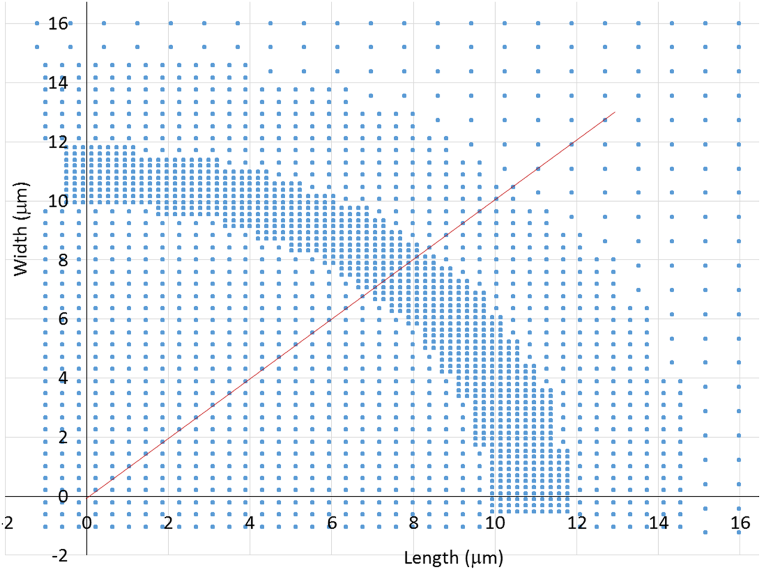
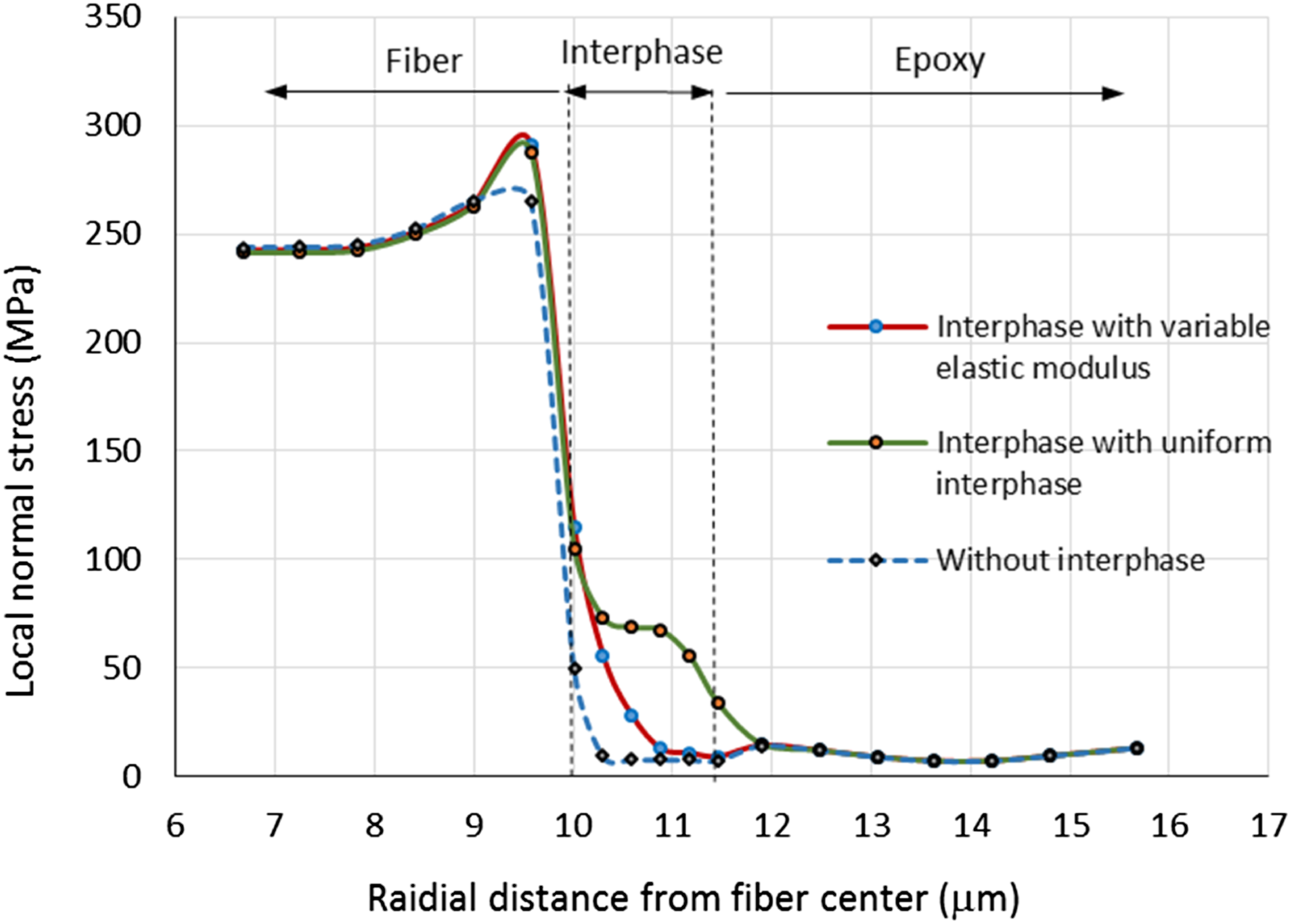
In Figures 29 and 30, variations of the obtained normal stresses are shown for specimens 4f and 3f, respectively. Figure 29 shows that there are sharp stress reductions at the interface of fiber and interphase region for the three hypotheses. But, at this interface the stress reaches point 1V (120 MPa) when the variable elastic modulus concept is used, point 1U (110 MPa) when the uniform elastic modulus concept is used, and point 1W (50 MPa) when the interphase region is ignored. The stress values are not significantly changed at the interphase region (about 75 MPa) when the uniform elastic modulus is considered at the interphase region. For the other two cases, the stresses reduce smoothly to stress values in the epoxy domain. The stress value of larger than 50 MPa is in the range of epoxy yield stress. Therefore, the obtained results reveal that the assumption of ignoring the interphase region may lead to non-conservative failure prediction, and using the concept of uniform interphase elastic modulus may lead to very conservative failure prediction in fiber/matrix interphase damage analyses when compared to the results for variable elastic modulus modelling. Almost the same stress behavior is visible for specimen 3f in Figure 30. Normal stress variation of the interphase in specimen 4f. Normal stress variation of the interphase in specimen 3f.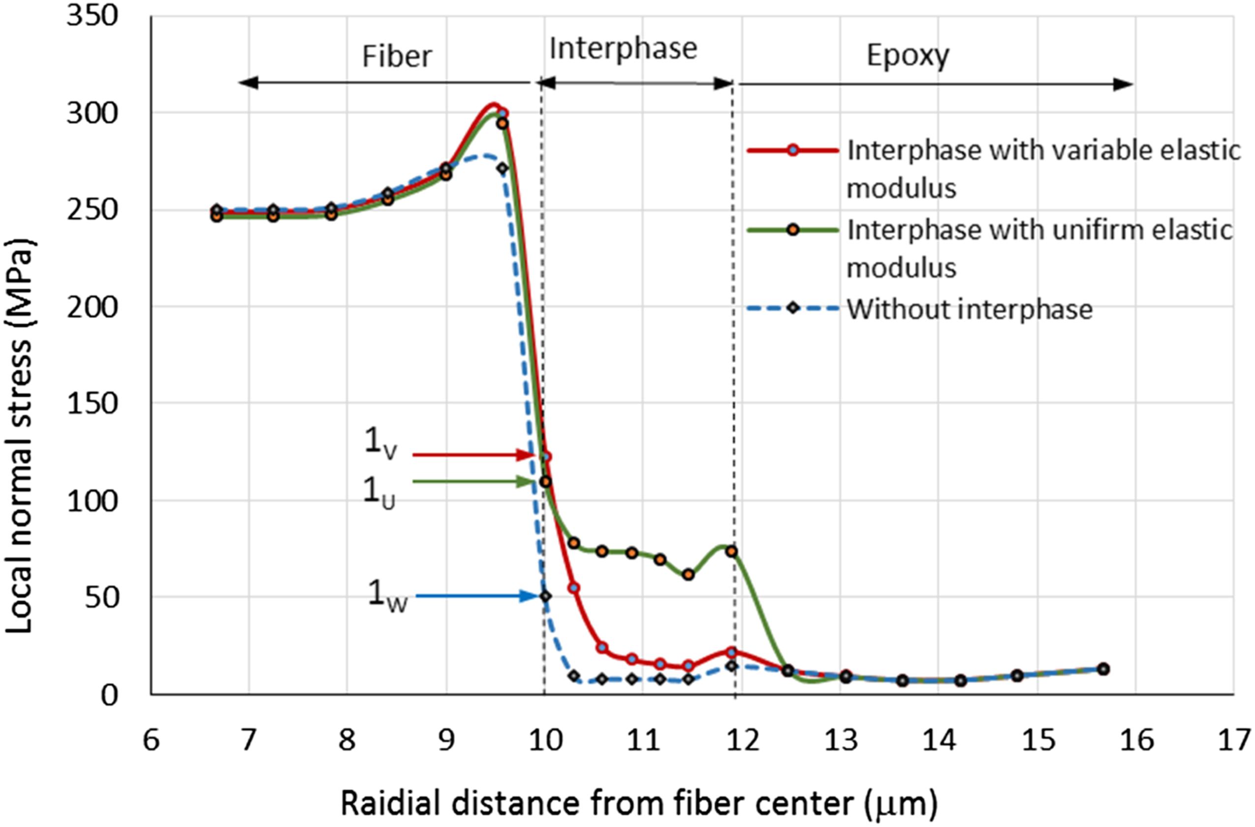
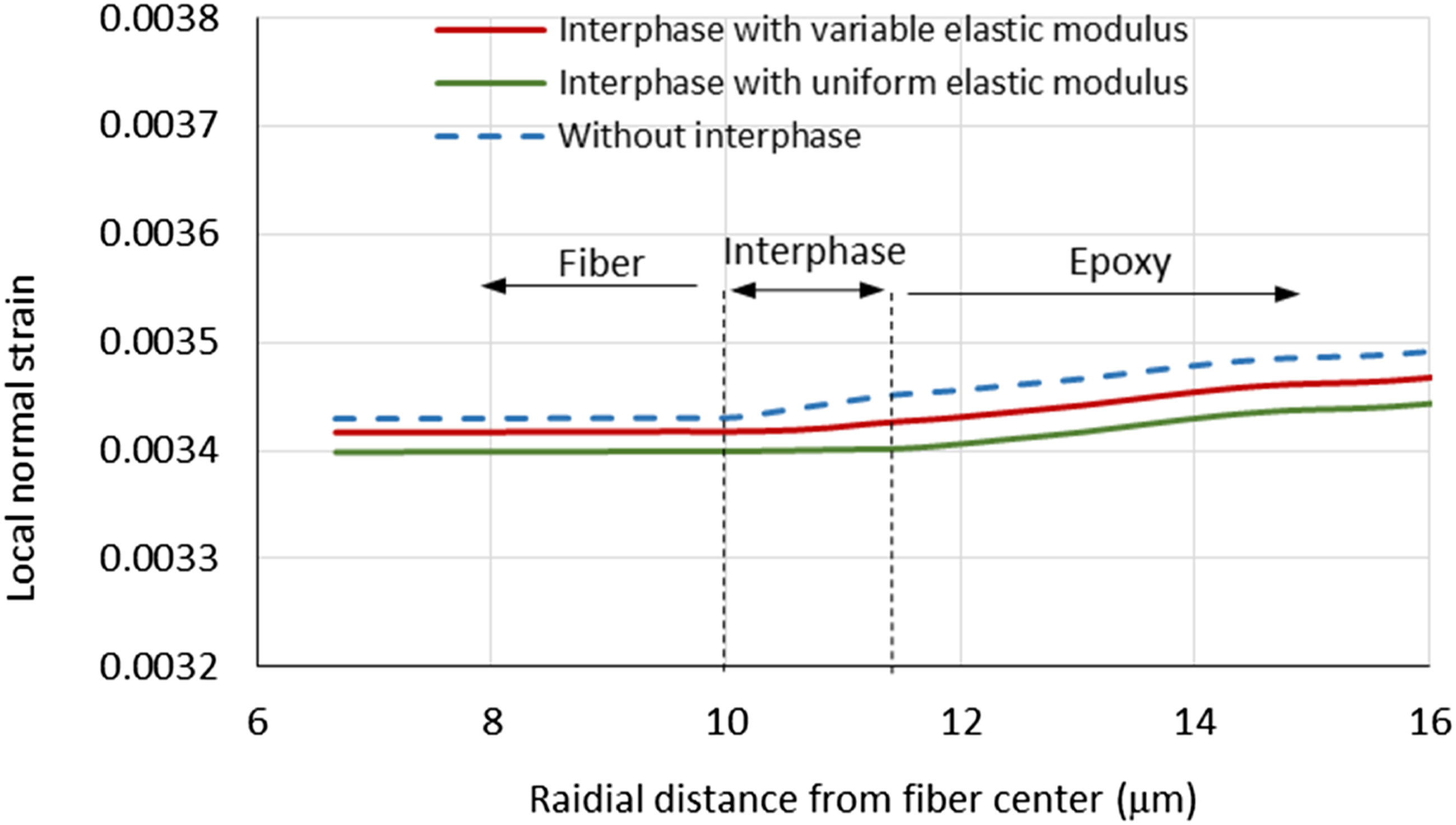
The obtained normal strains at interphase regions are shown in Figures 31 and 32 for specimens 4f and 3f, respectively. These figures show a smooth variation of normal strains along the radial direction from fiber to the epoxy domain for models with different concepts of interphase elastic modulus characterization. Also, the results show that in the model ignoring the interphase region, the strain is larger and increases in the epoxy region. However, in other models, the strain values at the interphase region are somehow close to those at fiber section strains. Strain variation of the interphase in specimen 4f. Strain variation of the interphase in specimen 3f.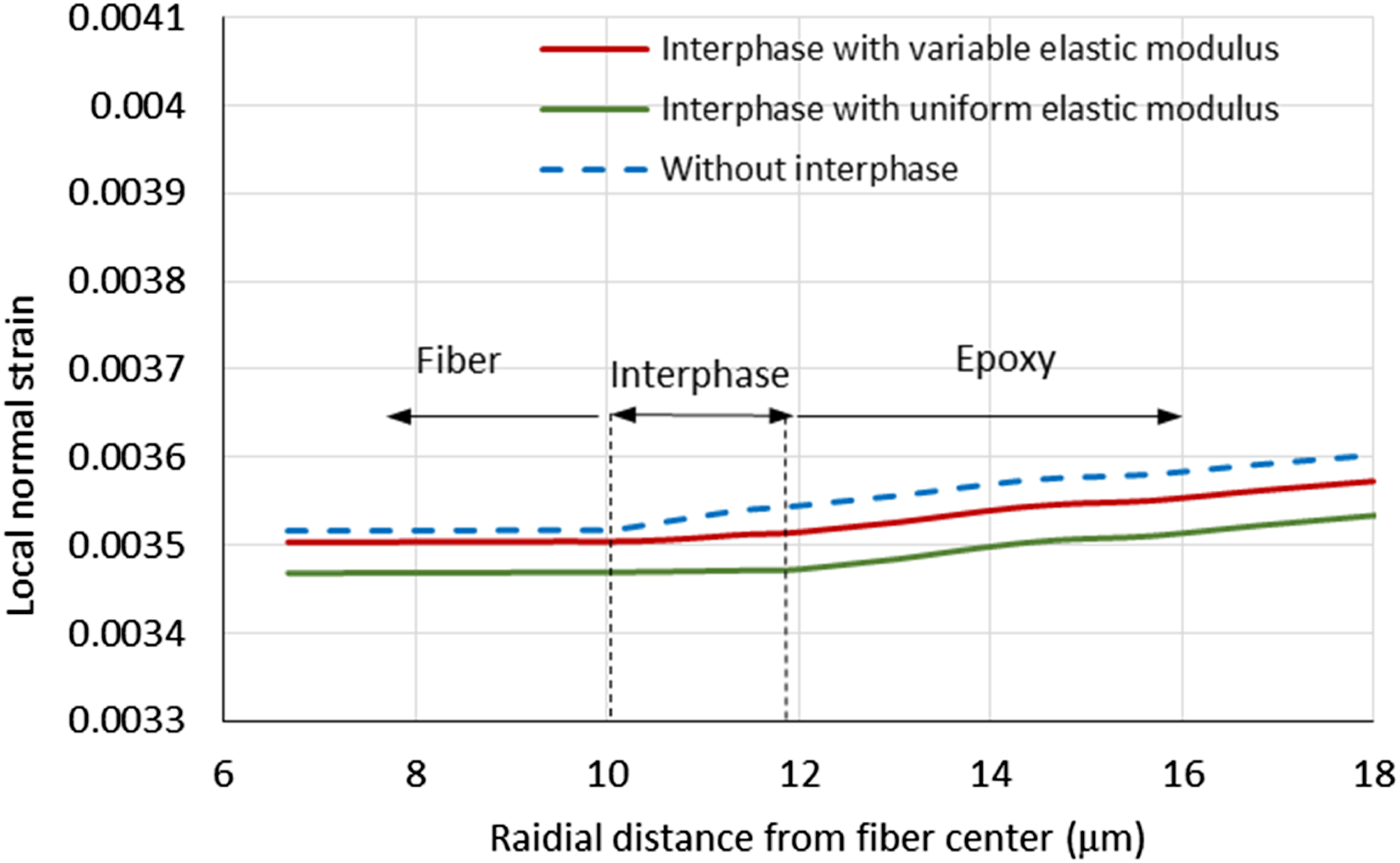
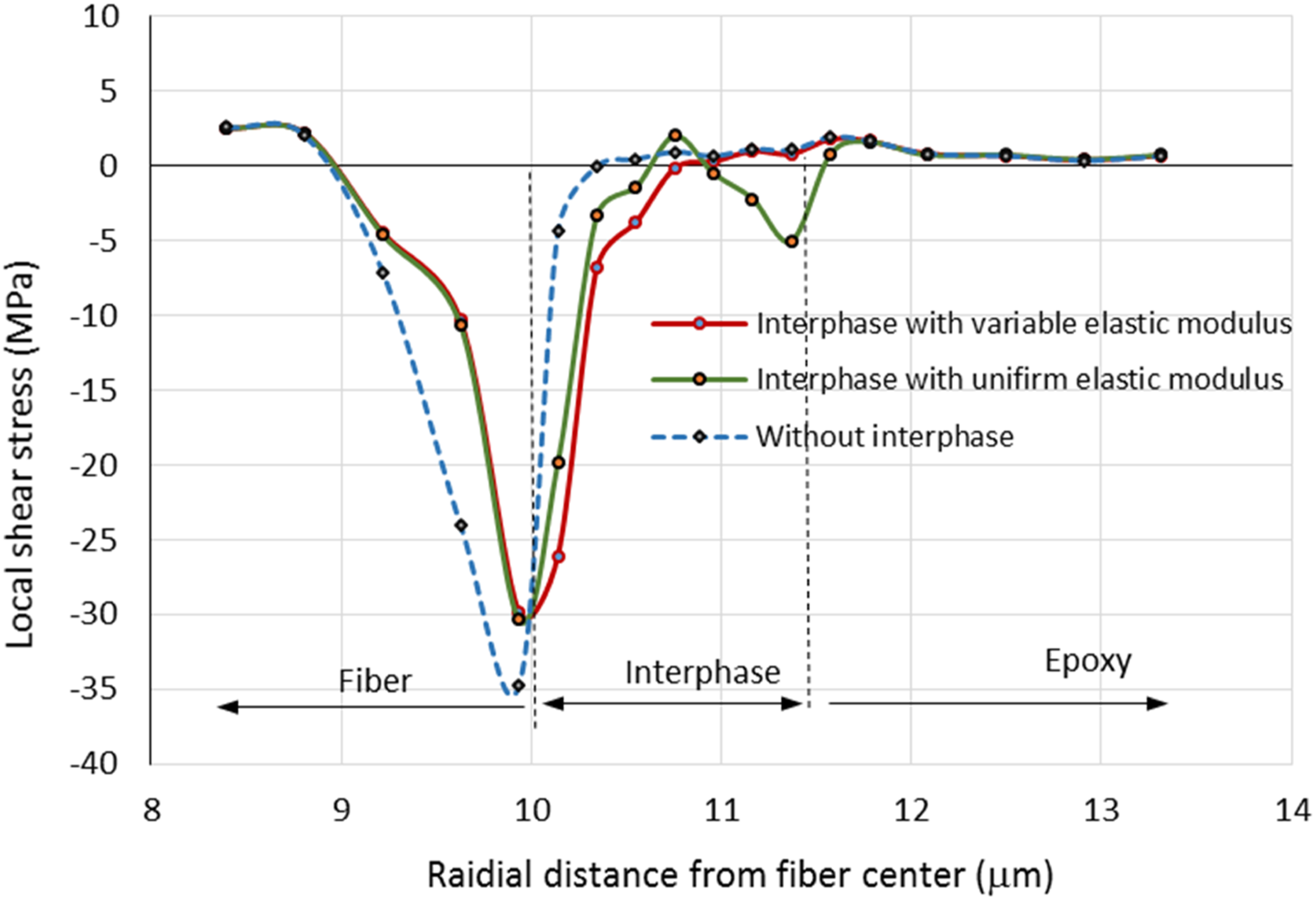
In Figures 33 and 34, variations of shear stresses in the z-direction (along loading) are depicted in different regions of the interphase and neighboring to the interphase. As expected, the shear stress at the interface of phases has a maximum local value with a jump. In both figures, the models ignoring the interphase region have larger values of shear stresses in the glass/epoxy interface with respect to the obtained shear stresses for uniform and variable elastic modulus models. This phenomenon comes from the significant difference in the mechanical properties of neighboring phases without the consideration of the interphase model. In uniform modelling of elastic property at interphase, there are two interfaces of fiber/interphase and interphase/epoxy regions. The obtained results also show two shear stress jumps at these interfaces. However, for the models with variable elastic modulus, the shear stress increases near the fiber/interphase boundary and gradually decreases to reach the minimum value close to zero. Shear stress variation of the interphase in specimen 4f. Shear stress variation of the interphase in specimen 3f.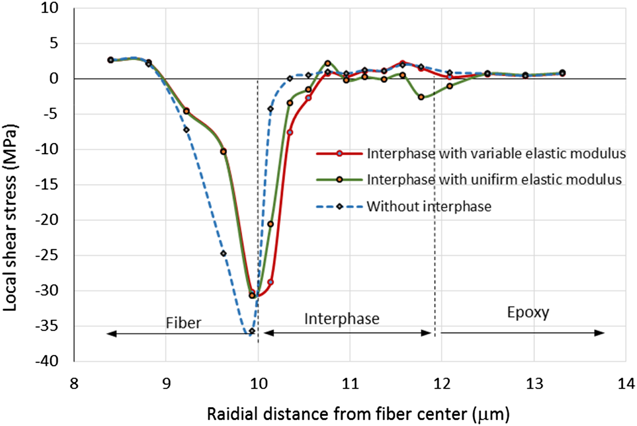
Conclusion
Usually, the traditional nano test methods, such as AFM and scratch testing, characterize the interphase at a specific region of the specimens. Different researchers have reported various interphase properties for the same composite materials. This diversity is due to the non-homogeneity of fiber coatings or weak chemical bonding in some specific locations on the fiber surface.
In this paper, we presented a method that calculated the overall interphase properties of FRP composites without the existing traditional restrictions. In this approach, the peridynamic method incorporated with an optimization technique, with the aid of micro tensile tests of single fiber specimens, was utilized to characterize the variation elastic modulus along the interphase region. The results showed that the interphase elastic modulus had the maximum value next to the fiber. In the first 200 nm from the fiber, the elastic modulus for different specimens was 40 ± 3 GPa. This value sharply decreased to reach the epoxy value at a distance of about 1.5 mm, known as the interphase thickness.
Comparison of the obtained variations of interphase elastic modulus with the available nano test results in the literature showed acceptable accuracy and validity of the developed procedure. The obtained variation of stresses showed that the assumption of ignoring the interphase region may lead to non-conservative failure prediction, and using the concept of uniform interphase elastic modulus may lead to very conservative failure prediction in fiber/matrix interphase damage analyses when compared to the results for variable elastic modulus modelling.
Footnotes
Declaration of conflicting interests
The author(s) declared no potential conflicts of interest with respect to the research, authorship, and/or publication of this article.
Funding
The author(s) received no financial support for the research, authorship, and/or publication of this article.