Sage Journals: Discover world-class research

Abstract

Amid rising concerns regarding student loan debt, we examine the effect of Washington State’s College Affordability Program introduced in 2015 on undergraduate student loan debt to provide policy-makers with additional tools to help prevent another student loan debt crisis. The program reduced tuition for resident full-time undergraduate students at public colleges and universities for two consecutive academic years. This policy adoption created a natural experiment that we exploit to identify a causal link between tuition and loans. Using college-level data for the 2009–2010 through 2021–2022 academic years and employing a difference-in-differences model in conjunction with nearest-neighbor matching, we show that a decrease in college tuition following the adoption of the College Affordability Program caused a $637.96 (9 percentage-point) decline in average loans among first-time, full-time undergraduates in Washington State relative to undergraduates from matched U.S. schools.

JEL Codes: G28, I22

Keywords

college tuition student loans state policy

Introduction

In the 1970s, the average tuition price was $5,000 a year, adjusting for inflation, compared to an average of $18,000 a year by 2019 (Abel and Deitz, 2019). With rising tuition, national student loan debt has steadily risen to an alarming $1.59 trillion in the first quarter of 2022 (Federal Reserve Bank of New York, 2022). Access to loans increases college enrollment and improves the odds of college completion by allowing students to pursue an education when the total cost is not within their current means. Notwithstanding these benefits, existing research has identified multiple adverse influences of student loans on post college outcomes, such as job choice and earnings (Daniels Jr & Smythe, 2019; Froidevaux et al., 2020), marriage (Bozick and Estacion, 2014), family formation, and net worth (Robb et al., 2019; Velez et al., 2019). Consequently, student loans not only contribute to lower discretionary spending but also generate negative externalities within communities. Given the far-reaching impact of student loan debt, we contribute to the discussions surrounding the growth in student loans by examining how much lower tuition can affect the demand for student loans.

Lowering tuition is often viewed as a direct and widespread means to increase college enrollment and completion rates. A few papers have gone beyond these immediate outcomes and focused on the relationship between tuition and student loans. Odle et al., 2021 use a difference-in-differences framework to examine the effect of lower college attendance costs due to Tennessee’s College Promise Program on the demand for student loans in community colleges. They find that this last-dollar program, covering 2 years (or 5 semesters) of tuition and mandatory fees, reduced the percentage of first-time students borrowing by 8–10 percentage points and reduced average loans by $230–360USD (nearly 32%). Chakrabarti et al., 2023 use administrative data to investigate the effect of higher university tuition on demand for graduate education and student loan debt, finding that a substantial increase in tuition of $5,000 leads to a $1,500 increase in total student debt. Bleemer et al., 2021 posit that recent student cohorts responded to tuition shocks not by forgoing college education but by amassing more debt.

Research and intuition tell us that higher tuition is associated with higher loans, but the relationship may be asymmetric; loans may respond differently to tuition decreases than to increases. Additionally, to prevent future student loan debt crises, policy-makers have advocated for lowering the cost of college attendance, and tuition-free public colleges are an increasingly popular idea (Siripurapu and Speier, 2021).¹ We contribute to the literature by examining a causal link between lower tuition and demand for student loans at public 4-year colleges using data from the 2009–2010 to 2021–2022 academic years.² While the effect of a lower cost of attendance at community colleges on loans is discussed in Odle et al., 2021, the estimated effect may not persist among students who experience smaller changes in tuition while enrolled in a 4-year program. Additionally, 4-year college programs often charge tuition that is more expensive than the sticker price associated with attending a community college and generally require a longer commitment before completion.

Using a structural model of higher education and the macroeconomy, Gordon and Hedlund, 2016 report that tuition increases in past years were mainly associated with increases in student borrowing limits and the persistent existence of college wage premiums. Lucca et al., 2019 use a difference-in-differences framework to analyze the effects of changes in federal loan program maximums to undergraduate students in the 2007–2008 and 2008–2009 academic years on college tuition and report a pass-through effect on tuition due to changes in subsidized loan maximums of approximately 60 cents on the dollar and approximately 20 cents on the dollar for unsubsidized federal loans. Because federal student loans represent only one of several funding sources used by college students, these results are quite salient. They suggest that credit expansions can impact tuition for a broad set of students, including those not receiving federal loans. Adding to the discussion with evidence from graduate programs, Kelchen, 2019 exploits a large increase in graduate student lending limits in 2006 to examine whether law schools responded by raising tuition. Although no substantial effect was identified on tuition at private law schools following the 2006 policy change, Kelchen, 2019 reports a modest increase in tuition and fees at public law schools. These results tend to confirm the Bennett Hypothesis: changes to loans may influence changes in tuition and vice versa. As a result, causal estimates of changes in tuition on student loans can only be uncovered if accommodations are made for simultaneity bias.

To isolate the effect of changes in tuition on student loans and minimize potential simultaneity issues, we use variations in tuition that resulted from legislative changes in the state of Washington. Using a difference-in-differences framework in conjunction with nearest-neighbor matching, we show that a decrease in college tuition following the adoption of the College Affordability Program caused a $637.96 (9-percentage-point) decline in average loans among first-time, full-time undergraduates in Washington State relative to undergraduates from matched U.S. schools. We also provide suggestive evidence of a reduction in the percentage of students who took out student loans.

There is growing concern about the increasing indebtedness of college graduates, as the cost of attending college has more than tripled since the 1970s. Since taking office in 2020, the Biden–Harris administration has provided some relief to borrowers through expanding federal student loan forgiveness programs. Although substantial, these efforts focus on the current student debt crisis without consideration for future loan increases. A longer-term solution is critical to abating student debt crises. Focusing on the root cause of student loan debt, our analysis provides additional tools for policy-makers focused on averting future debt crises.

The remainder of the paper proceeds as follows. Section 2 briefly discusses the College Affordability Program, and Section 3 provides details on the data. Section 4 describes the methodology, while Section 5 provides our main results and robustness checks. Section 6 concludes the paper.

Policy Background

On June 30, 2015, the Washington State Senate passed the Second Engrossed Substitute Senate Bill 5954 (the College Affordability Program) with unanimous support, which prompted statewide tuition reductions and placed limits on annual tuition increases (Washington State Senate, 2015). This policy reduced tuition rates for resident undergraduate students at public institutions of higher education for the 2015–2016 and 2016–2017 academic years.

Beginning in the 2018–2019 academic year, the College Affordability Program capped annual tuition increases at the average annual growth in median hourly wages. We can use this to deduce the underlying sentiments behind the policy and the factors that influenced its passing. Consider the standard hypothesis for the value of education: the choice to go to school is a function of the net return on education, calculated as the expected wages less the published tuition costs and future interest payments. The median hourly wage can be considered a conservative estimate of expected wages. As a result, restricting tuition increases to be at maximum the observed increase in the median wage of Washington residents would keep the college wage premium relatively stable and somewhat predictable, as the Truth in Tuition policy encourages. With this in mind, the College Affordability Program was designed to reduce tuition in Washington State and maintain stable growth over time. We propose that the policy also sought to bring the state’s average tuition rate closer to national levels.

The bill was introduced in February 2015 and passed at the end of June 2015, meaning students would only be able to take any anticipatory actions at the beginning of the spring quarter and would have no ability to react if their college operated on a semester schedule. Given the short period between announcement and approval, we argue that the policy’s announcement would not affect tuition or student financial aid since they are determined per academic year. In sum, we argue that the announcement of tuition reductions would not evoke in any student a change in behavior prior to the actual reductions in the 2015–2016 academic year.

The macroeconomic environment in which the policy passed was not particularly unique, which lends greater generalizability to the College Affordability Program. In Washington State, both the proportion of revenue from higher education to total revenue and the proportion of expenditures on higher education to total expenditures remain relatively constant every year (Figure A1), indicating no contemporaneous events that would influence tuition or loans besides the policy itself.

Tuition reductions for undergraduates at public 4-year institutions were not evenly distributed over two academic years. In the 2015–2016 academic year, full-time tuition fees for resident undergraduates at public universities and colleges experienced a 5% decline over the 2014–2015 rate, while reductions in the 2016–2017 academic year ranged from 15% to 20% lower than the 2014–2015 amount.³ It may be that the overall tuition level influenced voters and policy-makers to consider its reduction, but we would argue that this concern was not directly linked to changes in student loans. The College Affordability Program represents an exogenous change in tuition, so we can exploit the natural experiment to examine the causal link between tuition and the demand for student loans measured using average loan amounts and the proportion of first-time, full-time undergraduate student borrowers.

To provide more detailed institutional data, Appendix Table A1 shows tuition rates for the eight treated universities and the average tuition across community colleges in Washington State for 2013–2016. In Column 5, we compare tuition rates in the 2014 and 2016 academic years. This two-year difference in rates allows us to calculate the tuition savings due to the College Affordability Program. We find that tuition declined by 12%–16% at 4-year colleges, while the decline across community colleges was approximately 8% (see Column 6). This seems to suggest that declines in tuition at 4-year colleges were different in magnitude from the declines experienced at community colleges. A review of tuition across 4-year institutions further supports the claim that the treatment occurred in 2015 and not sooner. Relative to 2014, rates in 2015 declined across all institutions at an average rate of 3.2%. On the other hand, when we compared tuition rates across institutions in 2013 and 2014, tuition in 2014 increased, decreased, or remained largely unchanged.

Data

We utilize college-level data from public 4-year institutions across the United States to compare changes in student loans before and after the College Affordability Program was implemented in Washington State. Using the Department of Education’s Integrated Postsecondary Education Data System (IPEDS) (IPEDS, 2021), we collect institutional-level data for the academic years 2009–2010 through 2021–2022 to create a panel capturing six years before and six years after Washington adopted the tuition reduction policy.⁴ The 2015 College Affordability Program legislated tuition reduction at public postsecondary institutions (4-year colleges, as well as community and technical colleges) in Washington. However, our analysis focuses only on public 4-year programs because of the widespread adoption of community college promise programs. College promise programs vary across states but are geared toward providing tuition-free access to a 2-year college education. Since we are exploiting exogenous variation in tuition, the inclusion of these institutions may bias our results toward zero. For a similar reason, we exclude data from public 4-year institutions operating in the state of New York.⁵

The treatment group consists of eight public 4-year institutions operating in Washington. To assess the robustness of our results, we use multiple comparison groups. First, we rely on trends from colleges operating in all other states as our counterfactual. Second, we follow Hillman et al., 2015 and use data from colleges in states that are members of the Western Interstate Commission for Higher Education (WICHE) to create a control group. The WICHE includes Alaska, California, Colorado, Arizona, Hawaii, Idaho, Montana, North Dakota, Nevada, New Mexico, Oregon, South Dakota, Utah, Washington, and Wyoming. Third, we use the nearest-neighbor matching algorithm to identify colleges operating in other states that are observationally similar to 4-year institutions in Washington. Like Price & Surprenant, 2022, use 4 nearest-neighbor matches using propensity scores given evidence by Imbens, 2004 that matching parameter estimates are robust when selecting between 1 and 4 matches.⁶

Variables

There are four primary outcome variables: the log of average student loans, log tuition, the percentage of students holding federal loans, and the percentage of students holding nonfederal loans. Average loans reflect the average amount of student loans awarded to first-time, full-time degree/certificate-seeking undergraduate students. By tuition, we are referring to the in-district tuition price and fees for full-time undergraduate students. We also investigate changes in the percentage of first-time, full-time students borrowing federal loans and the percent borrowing other nonfederal loans.

Because student subgroups could respond differently to changes in the cost of college attendance, we include demographic controls, including the proportions of undergraduates enrolled that identify as Black, female, and Hispanic or Latino (Chen, 2008). For instance, the literature on the demand for student loans indicates that women and students of color are more likely to take out loans and in more significant amounts (Baker et al., 2017; Jackson and Reynolds, 2013; Miller, 2017).

Our financial controls include the percentage of full-time undergraduates awarded Pell Grants; the average federal, state, local, or institutional grant received by first-time, full-time degree/certificate-seeking undergraduate students; and the average spending on student services. Using the consumer price index, we account for inflation by converting all financial variables to 2019 dollars.

College quality can also have an indirect effect on the propensity to accumulate loans. Certain colleges are more likely than others to guarantee higher wages, offering greater incentives to take out more loans to endure higher tuition costs, but other aspects of a college campus and the experience of attending could produce similar responses. To account for institutional characteristics, we include the student‒faculty ratio, retention rates, 75th percentile of SAT math scores, whether SAT scores and high school’s national ranking are required for admission, and the institution’s location. Our analysis includes only SAT math scores, as the reading and writing sections were split from one section into two in 2016.⁷ The student‒faculty ratio is based on undergraduate students and primarily undergraduate teachers. Our location measure is based on an institution’s distance from the nearest principal city. Specifically, we use a categorical variable that captures schools in cities, towns, rural areas, and suburbs. Partly due to changes in population size, the value assigned to the location variable changed over the sample period for a few schools. As a result, we retain the initial classification for each institution. Summary statistics are presented in Table 1 for Washington and each comparison group separately. In Figure 1, we present p-values from the t-tests of differences in mean characteristics of the treated group and each control group.

Table 1.

Summary Statistics.

	Washington	All Other States	WICHE	Matched Control Group
	(1)	(2)	(3)	(4)
Financial Variables (2019$)
Published in-state tuition (per FTE)	10279.66 (1977.596)	9541.18 (2910.091)	8864.33 (2685.339)	9381.44 (2642.237)
Avg. loan amount	6062.62 (802.693)	6917.13 (1406.176)	6399.83 (1174.312)	7088.43 (1215.064)
Avg. grant amount	10014.99 (2904.939)	8743.48 (2900.576)	8843.75 (4216.545)	7712.64 (1868.776)
Avg. spending on students' services (per student)	1268.07 (686.988)	2087.95 (1027.322)	2462.85 (1059.184)	1485.59 (513.510)
Percent pell grant	.33 (.087)	.40 (.159)	.37 (.129)	.30 (.097)
Percent federal loans	.44 (.108)	.54 (.163)	.46 (.142)	.52 (.129)
Percent nonfederal loans	.02 (.016)	.06 (.058)	.04 (.048)	.07 (.051)
Avg. state funding per student	4854.07 (2670.261)	7295.27 (4290.489)	7593.90 (5280.223)	7046.42 (3856.958)
Demographic variables
Percent female	.53 (.027)	.55 (.089)	.53 (.084)	.55 (.058)
Percent Black	.04 (.020)	.15 (.214)	.03 (.021)	.04 (.025)
Percent Hispanic	.11 (.034)	.11 (.141)	.20 (.154)	.07 (.054)
Percent in city	.38 (.488)	.50 (.500)	.54 (.498)	.37 (.484)
Institutional characteristics
Student-faculty ratio	18.71 (2.645)	17.56 (3.630)	18.93 (4.384)	17.79 (2.861)
Retention rate	.79 (.078)	.76 (.102)	.77 (.100)	.78 (.086)
Test scores required	.91 (.286)	.88 (.320)	.83 (.376)	.88 (.329)
School rank required	.00 (.000)	.23 (.423)	.17 (.377)	.00 (.000)
SAT math score (75th percentile)	598.12 (53.986)	589.88 (66.773)	601.80 (61.969)	598.02 (44.818)
Observations	90	4444	920	381
Institutions	8	427	90	32

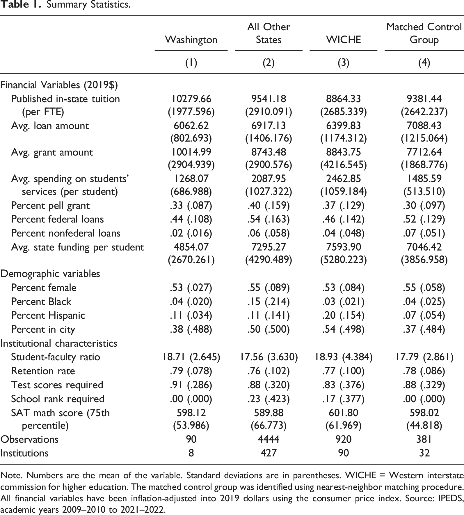
Note. Numbers are the mean of the variable. Standard deviations are in parentheses. WICHE = Western interstate commission for higher education. The matched control group was identified using nearest-neighbor matching procedure. All financial variables have been inflation-adjusted into 2019 dollars using the consumer price index. Source: IPEDS, academic years 2009–2010 to 2021–2022.

Figure 1.

T-tests for differences between Washington and alternate control groups.

Methodology

Simultaneity bias can obfuscate an estimate of the causal effect of changes in tuition on loans because changes in tuition may also be influenced by changes in loans (see, e.g., Kelchen, 2019). The 2015 College Affordability Program represents an event that decreased tuition independently of changes in loans. Including this event in a model instead of tuition itself allows us to estimate the effect tuition had on loans without bias from simultaneity.

Matching Procedure

To minimize concerns about bias from differential trends in tuition before 2015 between the treated schools in Washington and control schools in other states, we choose characteristically similar institutions using propensity scores and the nearest-neighbor matching procedure.⁸

The nearest-neighbor matching algorithm allows us to select four “nearest” control schools. When conducting the matching algorithm, we estimate propensity scores as the probability that a particular college is affected by the policy in Washington.⁹ After calculating propensity scores for each college in Washington, we use the nearest-neighbor matching method without replacement to select four unique control colleges with the most similar scores. The resulting five colleges (one treated and four controls) are given a label indicating their group g, and all unmatched colleges are removed from the analysis sample.

Propensity scores are estimated using the following school-level characteristics: location (city, rural, town, or suburb), whether the institution requires SAT scores or a student’s high school’s national ranking for admission, the share of female students, the percentage of Hispanic/Latino students, the share of African American students, the percentage of students receiving Pell grants, the student-to-faculty ratio, the average spending on student services, the retention rate, and the 75th percentile of SAT math scores. We measure these variables between 2009 and 2014, a year before the policy change.¹⁰

By including only colleges that are the most similar to the treated colleges in Washington, via observed factors, we reduce the confounding influence introduced by dissimilar colleges. Additionally, by including a group random effect parameter, we explicitly account for similarities in the outcome of the treated colleges and their matched counterparts. Figure A2 reports the absolute standardized mean difference in characteristics reported by institutions in Washington and the matched control group. This figure provides evidence that the differences in mean characteristics have mainly been reduced and become statistically insignificant after matching. When variables are still significantly different across the treated and control groups, they are accounted for in our difference-in-differences regression model as additional controls.

Difference-in-Differences Framework

We use a mixed-effects difference-in-differences framework to estimate the causal effect of tuition reduction on average student loan debt by comparing the change in average student loans in Washington State after relative to before the policy adoption to analogous changes in average student loans in control states. Our regression models take the following form

Y_{i s g t} = α_{s} + θ_{g} + λ_{t} + δ (T r e a t_{s} \times P o s t_{t}) + β x_{i s g t - k} + ϵ_{i s g t}

where Y_isgt represents our outcome variable of interest (the log of average student loans, log tuition, the percentage of students holding federal loans, and the percentage of students holding nonfederal loans) for university i in state s during academic year t within a matched group g. The product of Treat_s × Post_t is a binary indicator for Washington State (Treat_s) and post-policy years (Post_t), which takes a value of 1 for Washington in 2015 and later and 0 otherwise. The model includes state and year fixed effects denoted as α_s and λ_t, which capture state-invariant and time-invariant differences, respectively. Through matching, each treated institution is assigned a fixed number of untreated colleges—in our case, precisely four. The five units make up a matched group g, which we assume contains some unobserved similarities that the random effect, θ_g, captures.

Last, we include an additional control variable, x_isgt−k, which represents log average grants and log of state funding, depending on the dependent variable.¹¹ When a student decides how many loans they need to take out, they are very likely to first consider the amount of grant funding previously disbursed to them. In other words, the causal direction of grants on loans is relatively clear, as it seems illogical to accept fewer grants in response to more loans. Similarly, state funding impacts tuition levels, but not the other way around. In both cases, grants and state funding impact the demand for loans and tuition prices, but not the other way around; consequently, we account for these associations in our regression analysis.

The average treatment effect (ATE) is estimated by δ, which measures the difference in the change in tuition and loans in Washington following a policy change relative to the change in these outcomes among the control states. Standard errors are clustered by state.

Event Study Model

The validity of the average treatment effect estimate relies on the standard parallel trend assumption. In the absence of the tuition policy, we must assume that the loan amounts for colleges in Washington would have evolved similarly to loan amounts in the control group. Linear time, unfortunately, prevents any substantial proof of this assumption. To provide suggestive evidence that this assumption holds, we conduct an event study model of the following form

Y_{i s g t} = \sum_{t = - 4, t \neq - 1}^{4} γ_{t} T r e a t_{s} \times I_{t} + α_{s} + θ_{g} + λ_{t} + β x_{i s g t - k} + ϵ_{i s g t}

where each variable is defined the same as before. However, instead of estimating an average treatment effect across all post-tuition reduction policy years, a treatment effect γ_t is estimated for every year except one year before the policy was implemented. This is represented by the summation over pre-policy years (t < −1) and post-policy years (t ≥ 0) of the compound indicator variable Treat_s × I_t, which equals one when we observe a college in Washington during year t. Evidence for the parallel trends assumption is assessed by considering the statistical significance of each γ_t. The treatment effects for the pre-policy years are also called placebos, and the parallel trends assumption is supported when the placebo effects are not statistically significant.

Results

Table 1 presents descriptive statistics and compares the mean characteristics across schools in Washington against the national average, the WICHE averages, and the average across schools in our matched sample. An initial viewing suggests that the average experience of undergraduates attending 4-year public colleges in Washington State is different from the average experience of undergraduates attending schools in other states. For example, schools in Washington report higher average tuition and grants compared with the comparison groups. In terms of funding sources, higher grants in Washington are associated with a smaller proportion of the undergraduate population taking out federal and nonfederal loans and a smaller average loan amount.

In terms of demographics, the proportion of undergraduates who identify as Black or female in Washington is similar to that reported by schools in the match control group and the WICHE. However, Washington’s average proportion of female and Black students is lower than the national average. A similar pattern arises when we compare institutional characteristics, such as retention rate and SAT math scores: the averages reported by schools in Washington are more in line with the average across schools in the WICHE and the matched control group. These differences between Washington State schools and the national average motivate our decision to use additional counterfactual groups such as states from the WICHE as well as a matched control group in our analyses.

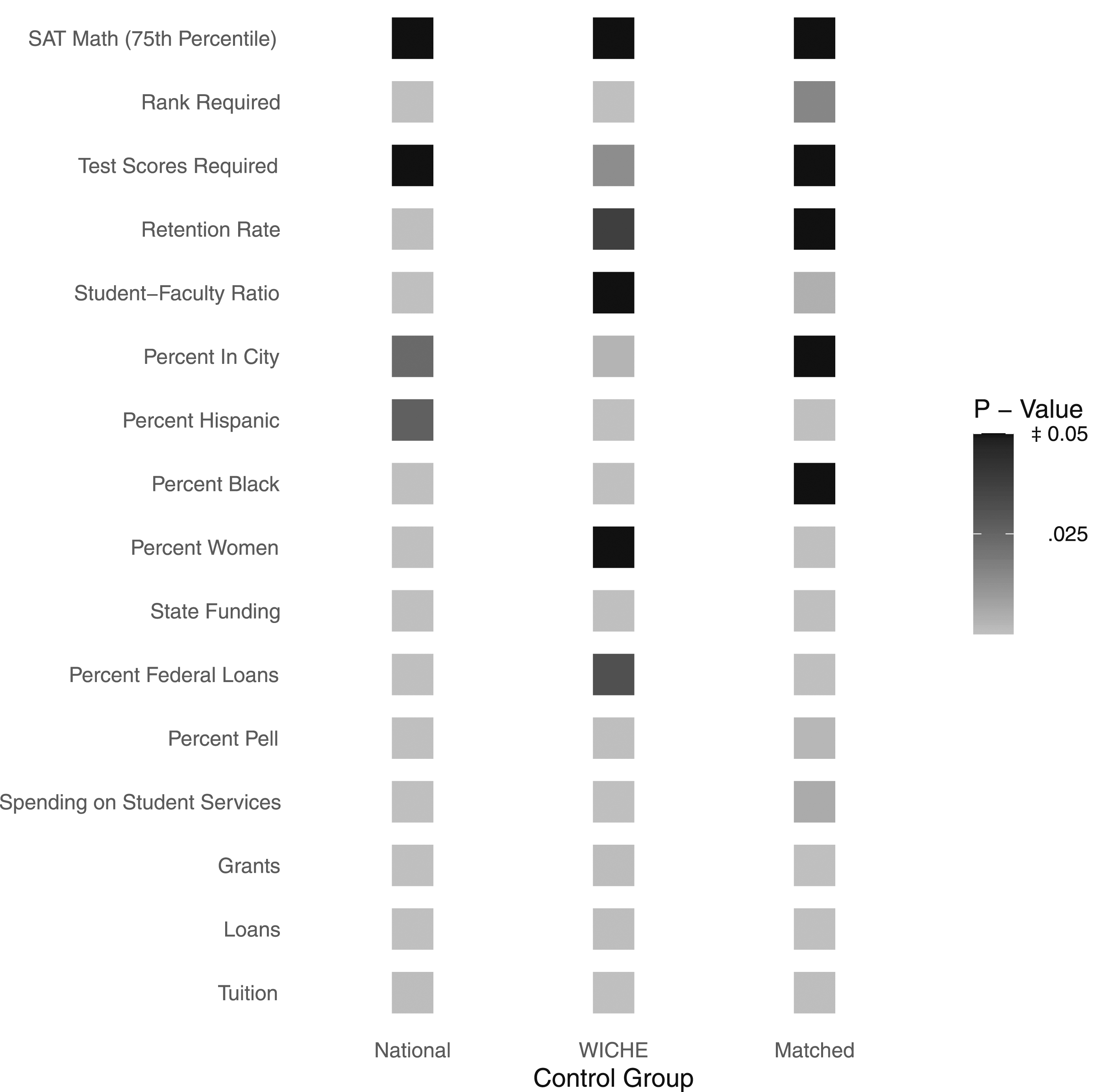
Figure 1 reports p-values from the test of differences in the mean characteristics reported by institutions in Washington and all three comparison groups. These results complement the summary statistics by revealing a significant difference between the characteristics reported by Washington and the average across all other states, with the exceptions of retention rates, SAT scores, test score requirement, and student‒faculty ratio. Of the 16 variables used to conduct our comparison, we only identify significant differences in five when we compare Washington to our matched control group. Consequently, Figure 1 provides evidence to suggest that through matching, we are able to use a sample of schools that compares well with schools in Washington.

Trends in Outcomes

Figures 2(a) and 2(b) present raw trends in average loans and tuition over a twelve-year period surrounding the tuition reduction policy for Washington and the three control groups.¹² The different broken lines represent trends across the control groups. Figure 2(a) confirms the pattern highlighted in Table 1. Washington had the lowest student loans on average. Figure 2(a) also shows that lower loans in Washington persisted over the sample period. While average loans for the national and matched control groups were substantially higher than loans reported in the treatment state, the average across states from the WICHE tracked well with the average for Washington. Although different in levels, the gap between the series remained relatively constant in the years before 2015, which indicates a parallel trend before the policy change. Notably, in 2016, loans in Washington State decreased, and they continued to fall until 2019. Loans increased briefly in 2020 before declining again in 2021. In 2017, average loans across the control groups increased briefly before largely decreasing over the remainder of the sample period.

Figure 2.

Raw trends in loans and tuition in Washington state and control groups.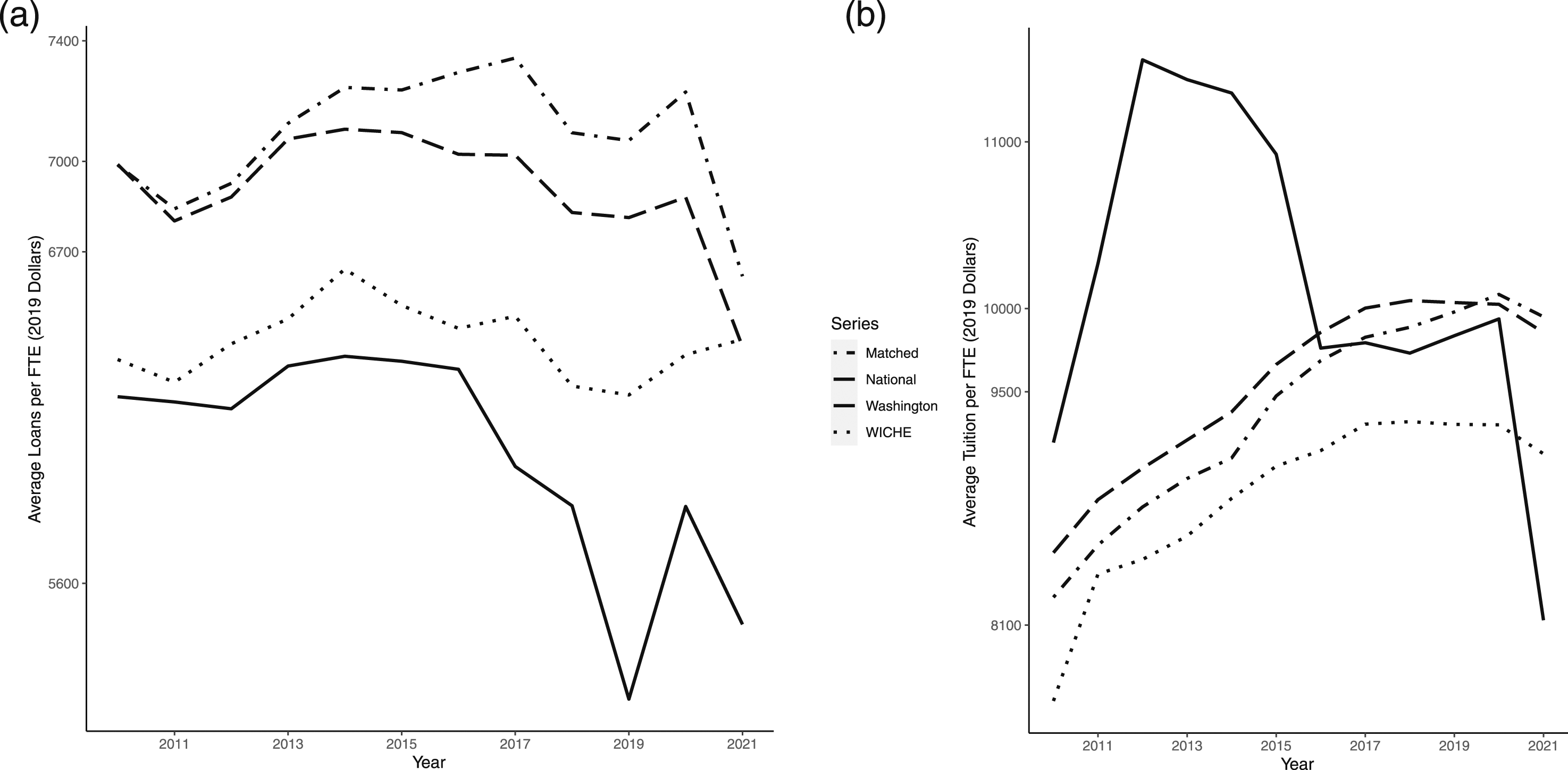

Figure 2(b) displays an upward trend in tuition across all groups in the pretreatment period, with Washington State reporting the highest tuition rates. Based on the figure, the average tuition for Washington declined in 2013, two years before the College Affordability Program was adopted. Although a larger decrease was observed in 2015, to ensure that our estimated treatment effect is not capturing changes unrelated to the 2015 law, we investigate alternate treatment dates in Section 5.3.

Figure 3 displays trends in average tuition, grants, and state funding in Washington over the sample period. Between 2009 and 2012, higher average tuition was associated with a decline in state funding. Post-2012, state funding increased, and average tuition fell as the economy recovered from the Great Recession. Given the inverse relationship between state funding and average tuition identified in Figure 3, we control for state funding in all our regression models analyzing changes in tuition.

Figure 3.

Raw trends in undergraduate tuition and select funding sources in Washington state.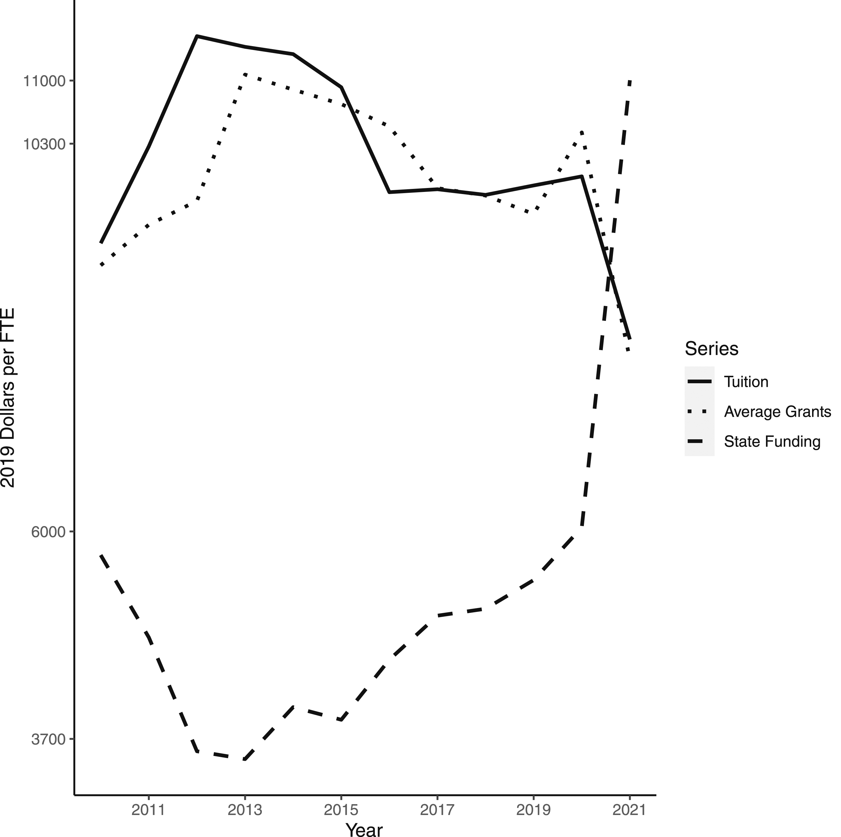

Overall, a comparison of the raw trend graphs provides suggestive evidence that (1) there were no substantial differences in the outcome variables before 2015, and (2) there was a change in the gap in outcomes after the tuition reduction policy was implemented in Washington State in the 2015–2016 academic year. Our event study models, shown in Figures 4(a) and 4(b), confirm that these conclusions hold once we account for covariates, state, and match-group fixed effects.

Figure 4.

Event studies for log tuition (a) and log loans (b).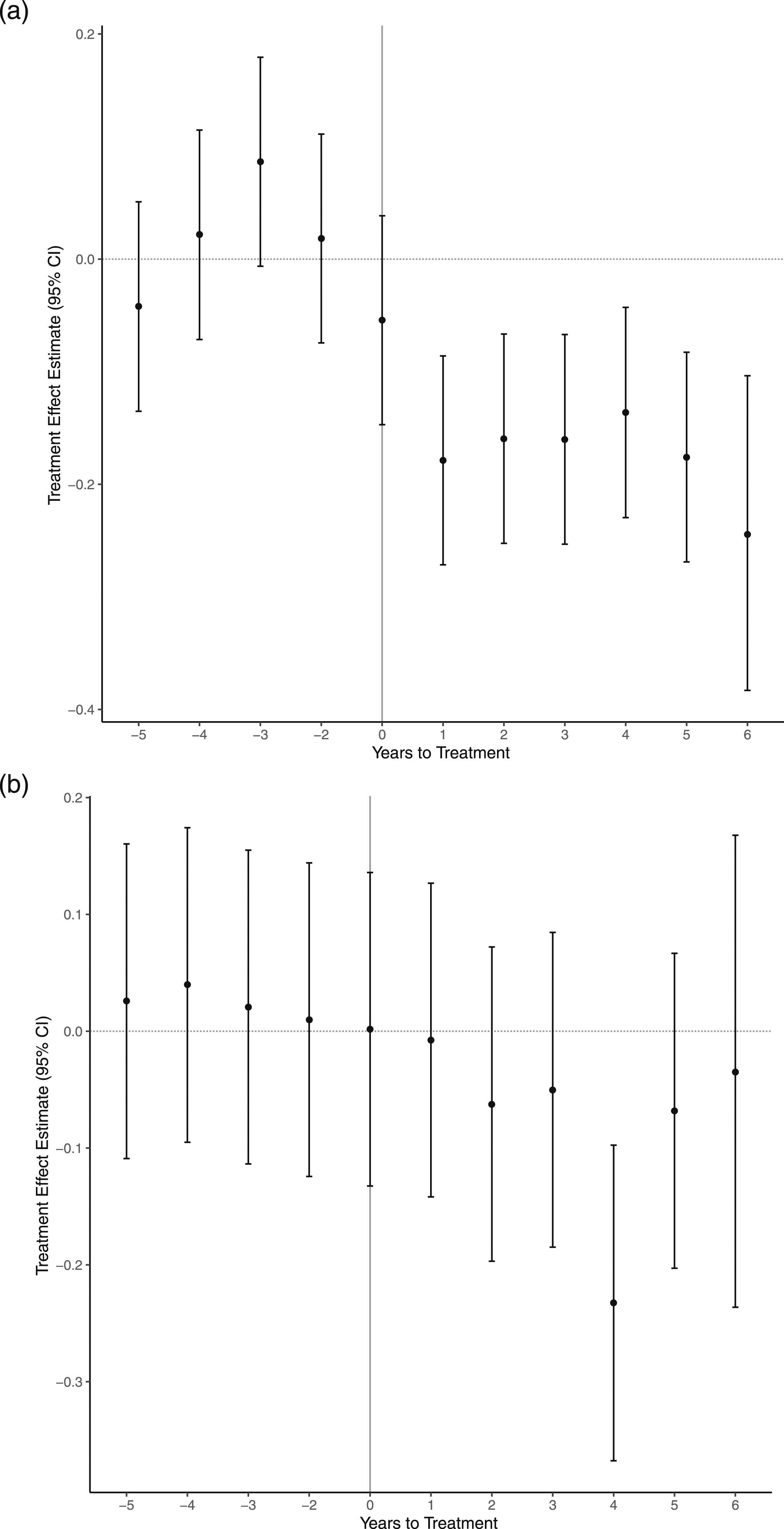

Figure A2 in the appendix plots the absolute standardized mean difference between the treatment and the matched control units for each matching variable.¹³ Overall, the difference in covariates (for the treated and control states) in the matched sample relative to the difference for the overall sample indicates that the matching algorithm has improved the sample balance. The difference in sample means seems to improve after matching, except concerning the variables pwomen and phispanic, which capture the proportions of students who identify as female and Hispanic, respectively. We include our matching variables as controls in all the models to ensure that the difference-in-differences results are not biased due to this estimated difference.

Regression Results

Irrespective of the control group, the results in Columns 1 through 3 of Table 2 suggest that the 2015 College Affordability Program caused a statistically significant decline in tuition at public 4-year colleges in Washington. The coefficient on (Treat × Post) ranges between −.19 and −.20, implying that the policy caused 19 to 20 percentage points in log tuition.

Table 2.

Difference-in-Differences Results for the College Affordability Program’s Impact on Tuition.

	Log Tuition			Log Loans
	National	WICHE	Matched	National	WICHE	Matched
	(1)	(2)	(3)	(4)	(5)	(6)
Treat x post	−.20***	−.20***	−.19***	−.05***	−.02	−.09**
	(.01)	(.01)	(.03)	(.01)	(.01)	(.03)
Log Grants_t						.07
						(.03)
Log Grants_t-1	.15**	.30**		−.04	−.01
	(.04)	(.08)		(.02)	(.06)
Log Grants_t-2	.13***	.10*		−.00	−.03
	(.02)	(.04)		(.02)	(.03)
Log state funding_t	.02	.02	.01	.01	.00
	(.02)	(.01)	(.01)	(.00)	(.01)
Log state Funding_t-1	−.01	−.01		−.00	−.01
	(.01)	(.01)		(.01)	(.02)
Year fixed effects	Yes	Yes	Yes	Yes	Yes	Yes
State fixed effects	Yes	Yes	Yes	Yes	Yes	Yes
Group random effects	No	No	Yes	No	No	Yes
Observations	3669	814	471	3669	814	471
Institutions	435	98	40	435	98	40

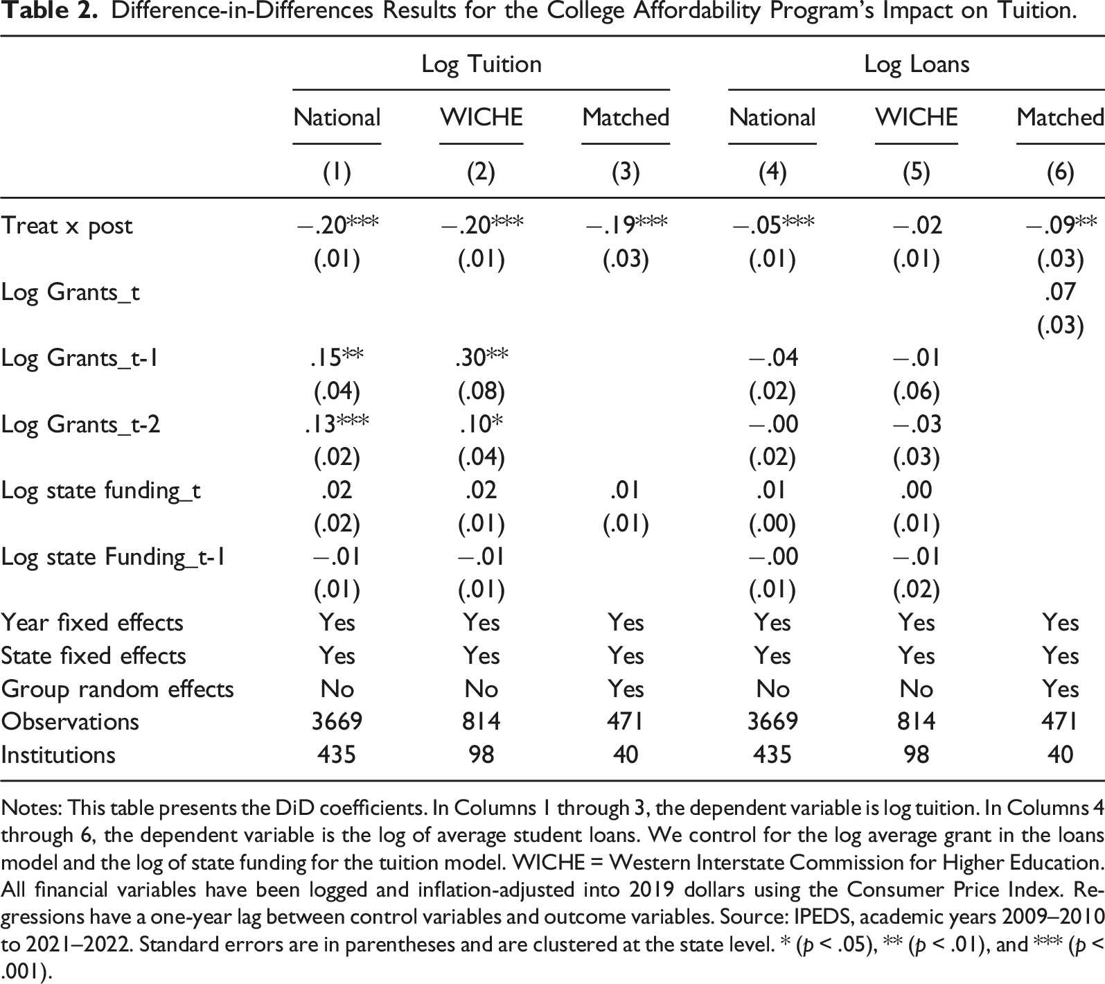
Notes: This table presents the DiD coefficients. In Columns 1 through 3, the dependent variable is log tuition. In Columns 4 through 6, the dependent variable is the log of average student loans. We control for the log average grant in the loans model and the log of state funding for the tuition model. WICHE = Western Interstate Commission for Higher Education. All financial variables have been logged and inflation-adjusted into 2019 dollars using the Consumer Price Index. Regressions have a one-year lag between control variables and outcome variables. Source: IPEDS, academic years 2009–2010 to 2021–2022. Standard errors are in parentheses and are clustered at the state level. * (p < .05), ** (p < .01), and *** (p < .001).

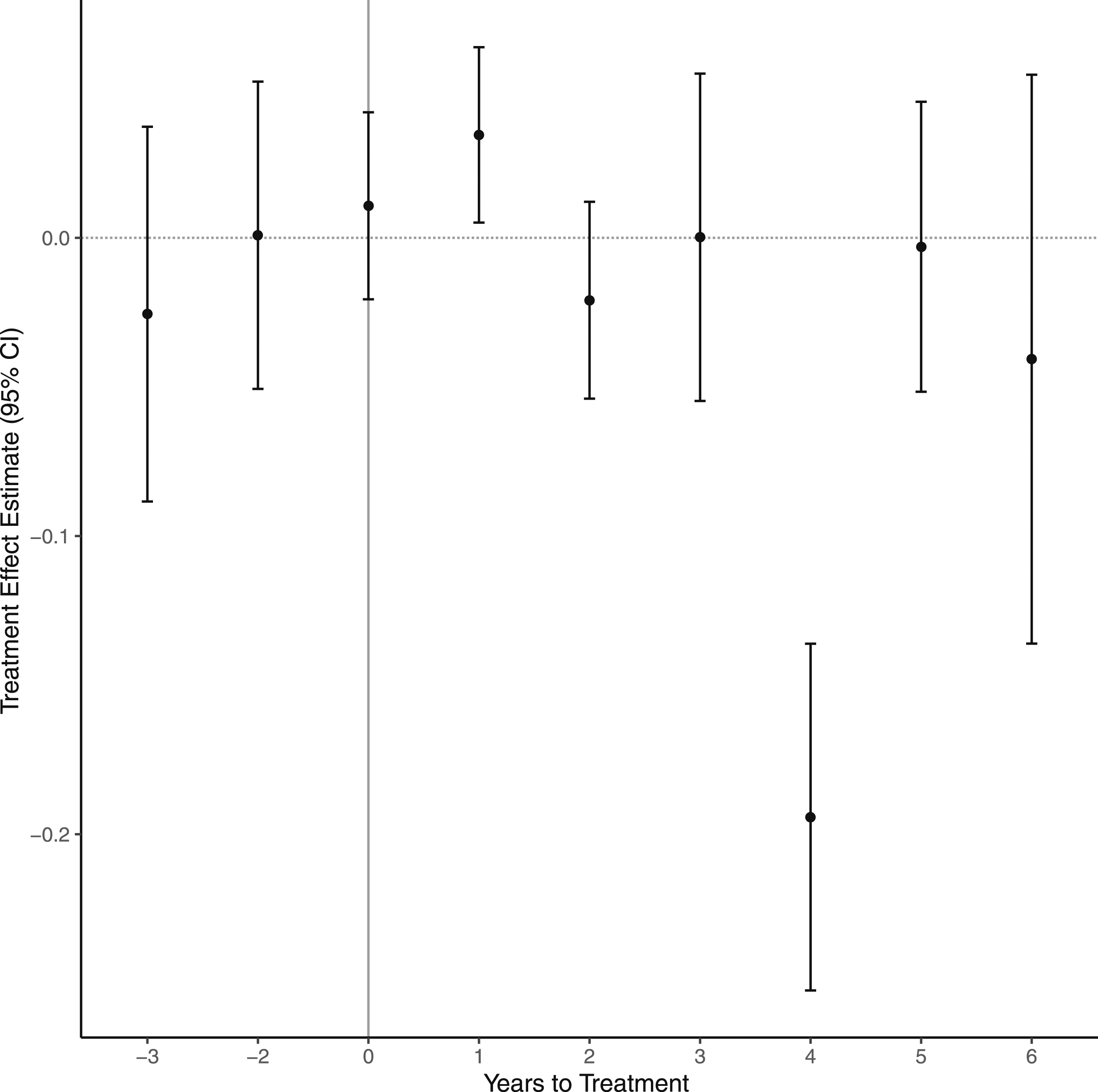
We use event study models to investigate the effect of the College Affordability Program over time by including leads and lags of our treatment variable, as outlined by equation (2). We consider five years before and six years after policy implementation in 2015. Figure 4(a) shows the results from the event studies for log tuition. This figure plots the coefficients on the interaction term between the indicator for the treatment state, Washington, and the indicators for each of the years before and after the policy adoption (γ_t), along with their associated 95% confidence intervals.

When we use our matched control group as a counterfactual for schools in Washington, we observe no evidence of any significant difference in log tuition between the treated and control groups before the policy adoption. This evidence supports the plausibility of the parallel trend assumption necessary for the validity of our difference-in-differences results. One year post-adoption (t = 1), we identify a statistically significant decrease in log tuition, which persists for the remainder of the sample period. Figure A3 and A4 display event study estimates for log tuition using schools in all other states or within the WICHE region as a control group. While Figure A3 displays negative and statistically significant treatment effects in the years after adoption, we observe evidence of a significant difference between Washington and all other states in the pretreatment years. As a result, Figure A3 provides evidence of no parallel trend pretreatment. While Figure A4 supports the parallel trend assumption, the post-estimation results suggest a significant increase in loan demand one year after adoption (t = 1) followed by a relative decline in subsequent years. Our matched control group is observationally similar to the treated institutions, so our matched analysis is preferred. Notably, however, similar to our matched analysis, Figure A4 suggests a significant decrease in loans four years after adoption (t = 4).

Columns 4 through 6 of Table 2 display the impact of the College Affordability Program on log loans. In terms of the sign and statistical significance of our treatment variable (Treat × Post), the results are broadly consistent across control groups, but the point estimates differ in terms of magnitude. The coefficient on Treat × Post, in Column 6, is −.09; this suggests that a fall in tuition due to the College Affordability Program caused a 9-percentage-point (approximately $637.96 from a baseline of $6,254.99) decline in log loans in Washington relative to average loans in the matched control group.¹⁴

This estimated decline of 9 percentage points compares well with the estimated 8–10-percentage-point decline in loans reported by Odle et al., 2021, due to the lower cost of college attendance from Tennessee’s College Promise Program. They estimated loan demand response to a change in tuition at 2-year community colleges in Tennessee, while we estimate a similar reaction to tuition declines at 4-year colleges in Washington state.

Figure 4(b) displays the estimated treatment effect for log loans over time and their respective 95% confidence intervals. Similar to the event study result for tuition in Figure 4(a), we find evidence that strongly supports the plausibility of the central identifying assumption of our difference-in-differences model. Although the individual event study coefficients in Figure 4(b) are not statistically significant until four years post-adoption, they demonstrate a persistent decrease in log loans for all six years.

Across Table 2, we show that a decrease in log tuition because of the 2015 College Affordability Program caused a statistically significant decline in log student loans. Estimates in Table 3 suggest that the tuition reduction policy caused significant declines in the percentage of first-time, full-time students who take out student loans.¹⁵ Relative to the matched control group, the percentage of students taking out federal and nonfederal loans in Washington State declined by three and two percentage points, respectively. The significant decline in nonfederal student loans is not surprising since these loans attract higher interest payments than federal loans. Figures 5(a) and 5(b) display the event study results for federal and nonfederal loans. Both show no significant difference across treated and matched controlled colleges before the policy change in 2015. These results provide suggestive evidence that the parallel trend assumption needed for difference-in-differences models is not violated.

Table 3.

Difference-in-Differences Results for the College Affordability Program’s Impact on Average Student Loans.

	Percent fed. Loans	Percent Non-fed. Loans
	(1)	(2)
Treat X Post (all other states)	−.01	−.01**
	(.00)	(.00)
Treat X Post (WICHE)	−.01	−.01
	(.01)	(.00)
Treat X Post (matched control group)	−.03	−.02***
	(.02)	(.01)

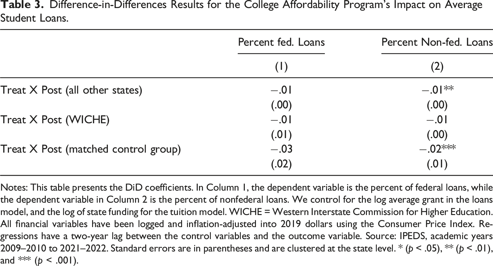
Notes: This table presents the DiD coefficients. In Column 1, the dependent variable is the percent of federal loans, while the dependent variable in Column 2 is the percent of nonfederal loans. We control for the log average grant in the loans model, and the log of state funding for the tuition model. WICHE = Western Interstate Commission for Higher Education. All financial variables have been logged and inflation-adjusted into 2019 dollars using the Consumer Price Index. Regressions have a two-year lag between the control variables and the outcome variable. Source: IPEDS, academic years 2009–2010 to 2021–2022. Standard errors are in parentheses and are clustered at the state level. * (p < .05), ** (p < .01), and *** (p < .001).

Figure 5.

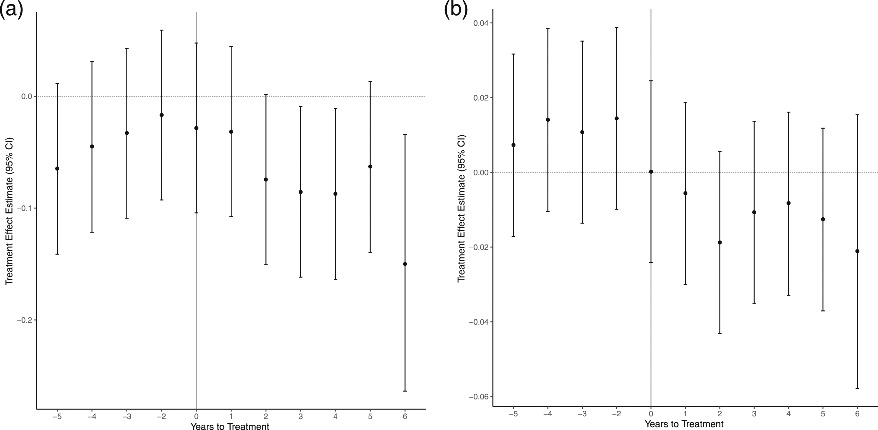
Event studies for percent federal (a) and nonfederal (b) loans.

Robustness of Regression Results

In this section, we discuss the results of some robustness checks. The aim is to assess whether the estimates presented in Tables 2 and 3 are sensitive to several specification issues. Our main results were obtained through an approach designed to maximize internal validity. Matching, the difference-in-differences framework, and the event studies model are expected to minimize the potential simultaneity bias present when considering the relationship between tuition and student loans. Nevertheless, there is the question of whether our estimate reflects the causal effect of a reduction in tuition on demand for student loans.

Statistical power is a potential issue when using the relatively small sample for our matched difference-in-differences estimation, given the number of parameters estimated. However, Dziak et al. (2020) argue against post hoc power analyses in general, especially when examining the power of a statistical model to detect an observed effect. Our goal, instead, is to determine the limits of what our analysis can achieve. Because we use a mixed-effects model, we estimate the statistical power through simulation techniques. Figure 6 displays the power of the model of log of loans with matched data to detect an ATE of −.07 by varying the number of institutions involved. In the primary analysis, we have eight treated institutions and 32 control institutions, which corresponds to 32 on the x-axis. The number of control institutions is varied one-to-one with the x-axis, while the number of treated institutions only increases one by one from eight to sixteen. Figure 6 shows that, at minimum, an ATE of −.07 can be detected with 80% power using approximately 20 control institutions and 8 treated institutions.

Figure 6.

Statistical power of log loans model with matched control group for different sample sizes.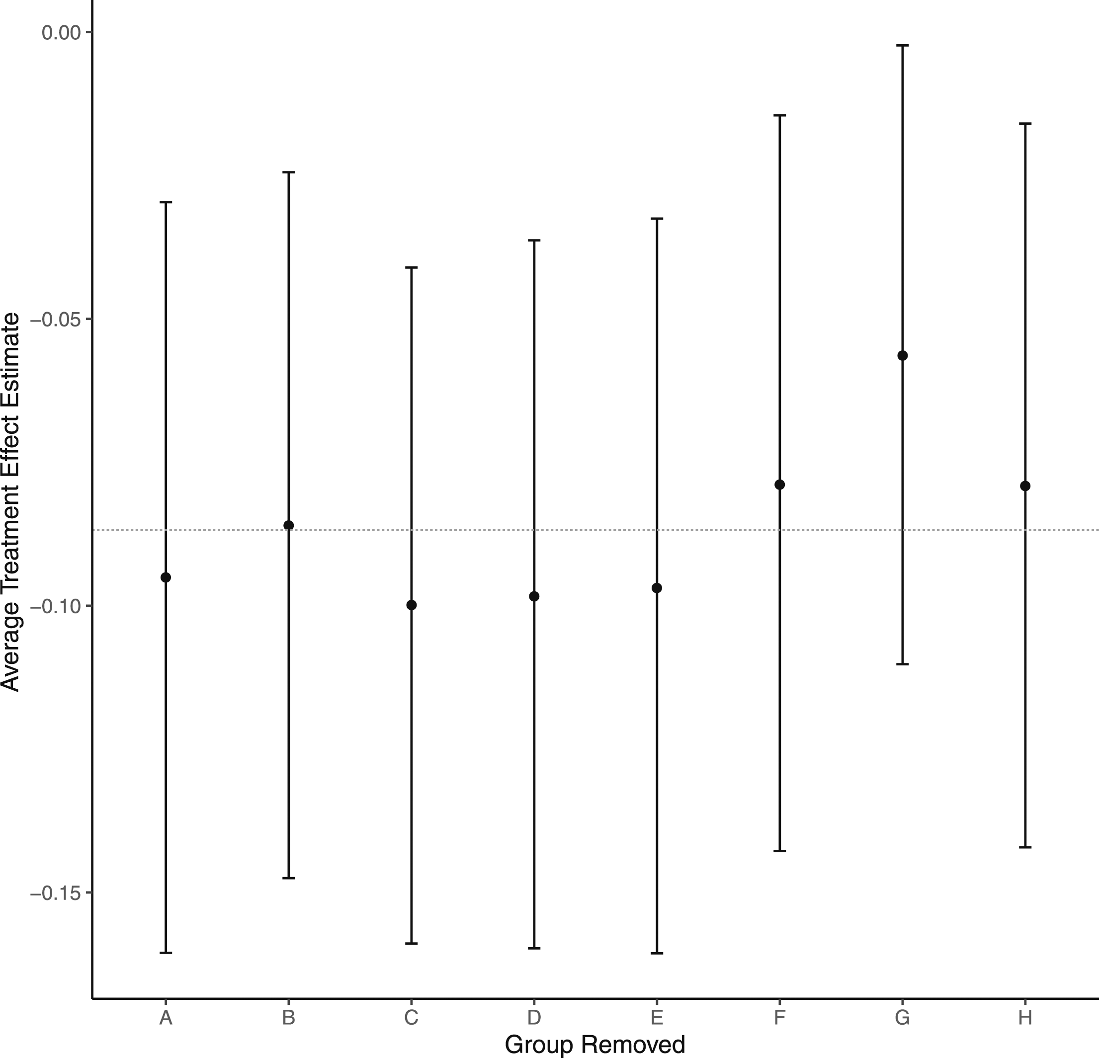

To check that the estimated effect is due to the 2015 decline in tuition and not some alternate shock, we manipulate the treatment year. The objective is to test whether the false treatment year replicates the main results. We construct a new sample in the same fashion as our primary analysis data but use university-level data from 2009 to 2014 rather than from 2009 to 2021.¹⁶ With this new analysis sample, we create a new posttreatment variable that dictates that public 4-year universities in Washington decreased tuition in 2012 instead of 2015. The estimated treatment effect for this redefined sample was δ = −.0342, p = .288. This insignificant result supports our claim that the estimated decline in student loans is due to the 2015 exogenous shock to tuition and not some alternate reason.

A review of the literature on the demand for postsecondary education reveals that rising unemployment can send a nonprice signal to individuals (both unemployed and employed), which motivates investment in human capital to prepare for changes in the labor market (Barr and Turner, 2015; Betts and McFarland, 1995; Dunbar et al., 2011; Hillman and Orians, 2013; Mullin and Phillippe, 2009). Focusing on enrollment at community colleges, Hillman and Orians, 2013 provide evidence that demand for college is countercyclical to changes in the labor market. Specifically, their findings indicate that a one-percentage-point change in the state unemployment rate is associated with a 1.1−3.3% increase in enrollment. Against this background, we modify our main model to include the state unemployment rate. As the unemployment rate rises, the opportunity cost of attending college should decline. As a result, more individuals will invest in college education, which must often be funded partly with student loans. This supports a positive link between unemployment and demand for student loans and is supported by our results in Table A2. Using the matched control group as a counterfactual for Washington in our analysis, Table A2 demonstrates a positive relationship between unemployment rates and log loans. Accounting for the state unemployment rate in our estimation does not substantially change our main result that an exogenous reduction in tuition due to the College Affordability Program in Washington State caused a decline in average student loans.

We perform a kind of cross-validation using the matched control group. Instead of the traditional method of removing a fixed number of observations at random and re-estimating, as this could disrupt the balance of the sample, we remove an entire matched group and re-estimate the difference-in-differences model. This maintains the same ratio between treated and control colleges and offers a way to determine whether a single treated college is driving the overall estimate. Figure A4 illustrates the estimated treatment effects along with the associated 95% confidence intervals. We also include a broken line at −.09 to highlight our main causal estimate from Table 2. In general, the matched group cross-validation performs well. Each individual difference-in-differences coefficient is negative and not significantly different from the main result. This seems to suggest that our main result does not reflect heterogeneous treatment effects associated with one or more treated units in our sample.

Given that the treatment effect estimated using a difference-in-differences model relies heavily on the parallel trend assumption, we complement our main estimation strategy with a matching estimator. Consistent with our main model, we use propensity scores to determine the nearest-neighbor as the distance metric to estimate the treatment parameter with four matches. Our results suggest an average treatment effect of −.064 with a bootstrapped 95% confidence interval of −.053 to −.079. This treatment parameter indicates that lower tuition caused a significant decline of 6.4 percentage points in demand for loans among students in Washington relative to loan demand by students in observationally similar schools. Most importantly, this estimated effect is relatively close to our main result.

Conclusion

We use a difference-in-differences model in conjunction with nearest-neighbor matching to show that a decrease in college tuition following the adoption of the College Affordability Program caused a reduction in the average loan amount taken out by undergraduate students. A positive correlation is not unexpected, but we argue that the causal effect of tuition on student loans requires a more nuanced model. The purpose of including matching and a causal framework was to strengthen our claims on the sensitivity of student loan changes in response to exogenous shocks to tuition. This approach limits bias and strengthens our study’s internal validity.

The sensitivity of the response of student loans to tuition is relatively inelastic. Using the ATE on log loans of −.09 and the ATE on log tuition of −.19, a back-of-the-envelope calculation returns an elasticity of .47. Possible economic explanations for the relatively low response of loans to changes in tuition may be associated with expectations of higher tuition or housing costs in later years, given that these costs generally do not fall over the long run. Conversely, some students may believe a drop in tuition would allow them to spend more on other kinds of consumption. However, our findings do not reveal the motivations for the response we have observed, so we do not attempt further conjecture in this area.

The descriptive analysis outlined in Macy and Terry, 2007 implies that tuition reductions are one of the most effective ways to combat student debt. Odle et al., 2021 show that the decrease in the cost of community college attendance due to the Tennessee Promise program caused a decline in demand for student loans. We add to the discussion by providing evidence of a causal link between tuition reduction at 4-year colleges in Washington State and the demand for student loans. Specifically, we use data from 2009 to 2021 to show that a decrease in college tuition following the adoption of the College Affordability Program caused a $637.96 (9-percentage-point) decline in average loans among first-time, full-time undergraduates in Washington State relative to undergraduates from matched U.S. schools. Given our results, the next relevant question will be how individual colleges handle tuition reductions. Tuition reductions of any magnitude could potentially jeopardize colleges’ budgets, especially those operating at or near zero economic profit, such as public colleges. With this in mind, future research must consider how funds would be reallocated and identify economically feasible tuition reduction levels.

One drawback to our empirical framework is that we sacrifice generalizability by attempting to maximize internal validity. To assess the robustness of our results, we estimate our model with three different samples, and our results do not vary much across samples. While we are confident that the matched sample offered the most unbiased causal estimate, we can see that the larger regional sample still produced statistically significant and adverse treatment effects.

Future work examining how loan responses vary with students’ socioeconomic profiles would be pertinent and may be achieved with more administrative, student-level data.

Footnotes

Declaration of Conflicting Interests

The author(s) declared no potential conflicts of interest with respect to the research, authorship, and/or publication of this article.

Funding

The author(s) received no financial support for the research, authorship, and/or publication of this article.

ORCID iDs

Zachary Jacob Dowdy

Tennecia Dacass

Notes

Appendix A. Proportion of Revenue and Expenses from and on Higher Education.

The following figure displays State expenditures on higher education and State revenue from higher education as proportions of total expenditures and total revenue, respectively.

Figure A1.

State revenue and expenditures from and on higher education as a percentage of total state revenue and expenditures.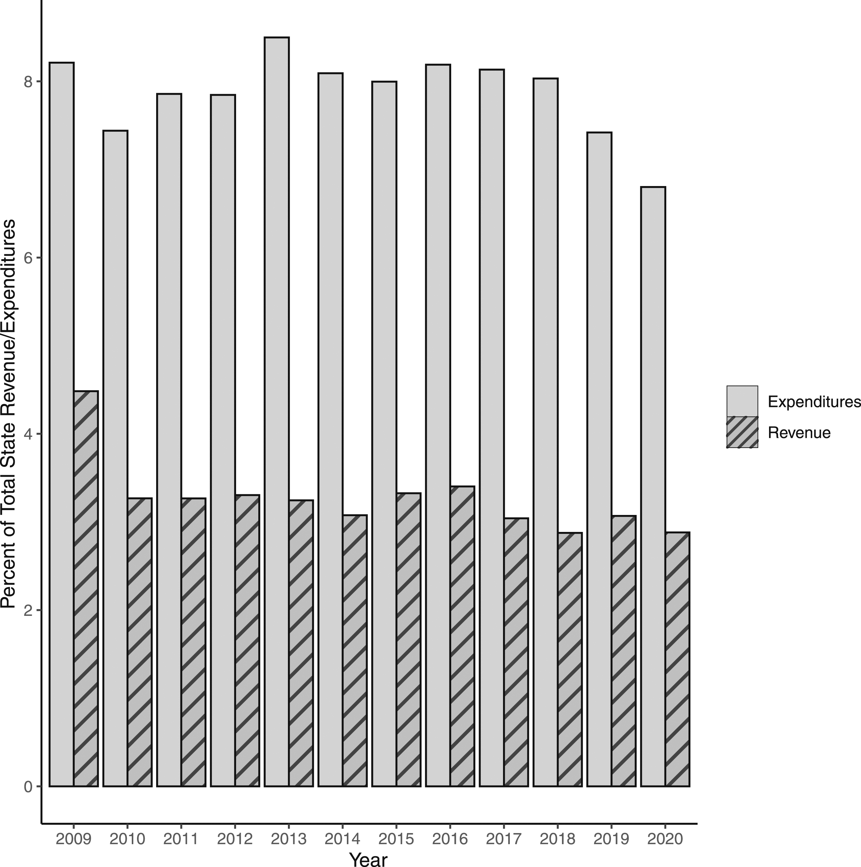

Appendix B. Assessment of Balance after Matching.

Figure A2.

Assessment of balance after matching.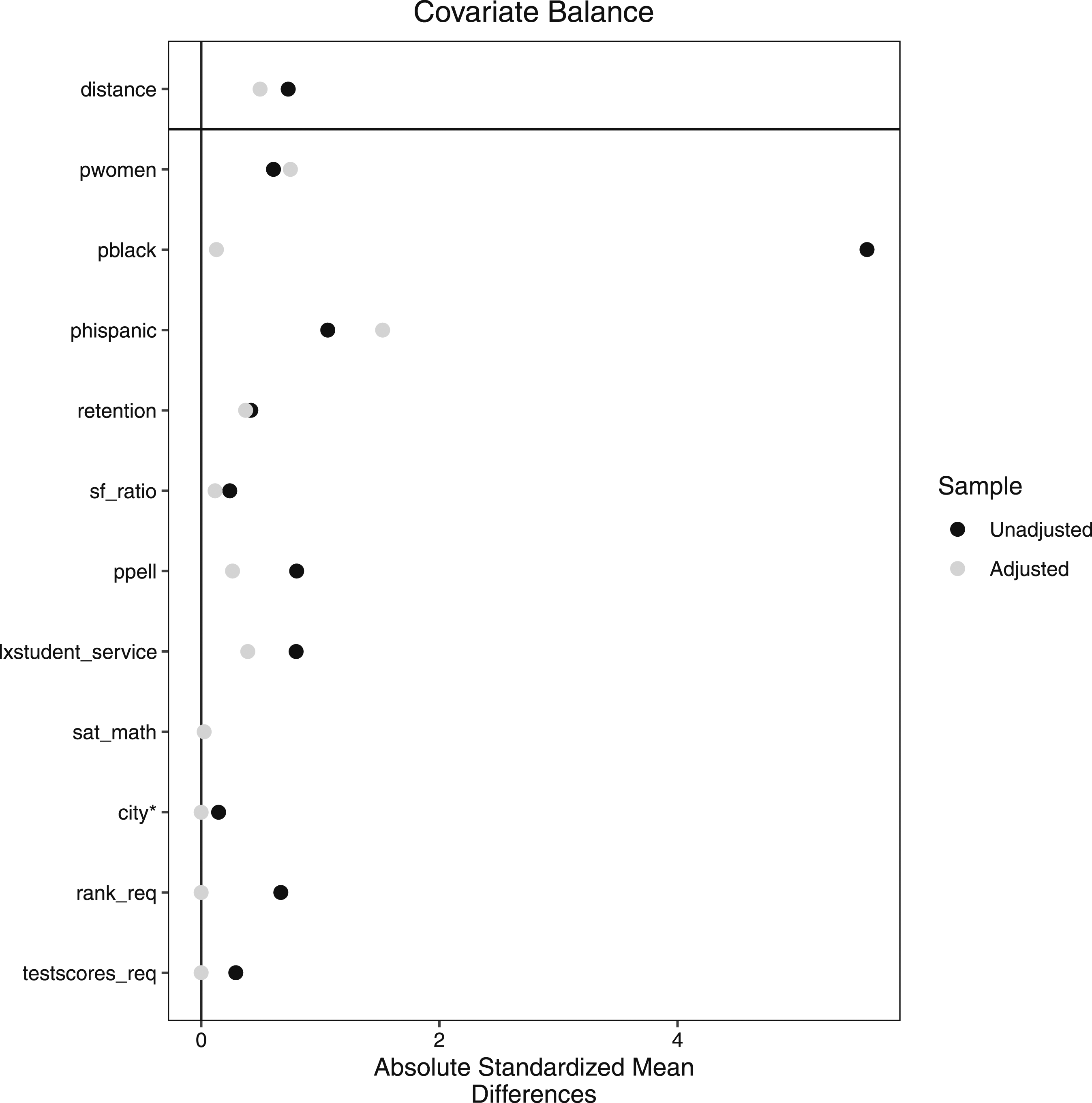

Appendix C. Event Studies for Alternate Control Groups.

Event studies were conducted to assess whether parallel trends would still hold for the national sample of U.S. colleges or the WICHE state colleges as control groups. The results outlined in Figure A3 and A4 indicate that the parallel trends assumption likely does not hold when using these different control groups.

Figure A3.

Event study for log loans using all other US. states as a control group.

Figure A4.

Event study for log loans using WICHE states as a control group.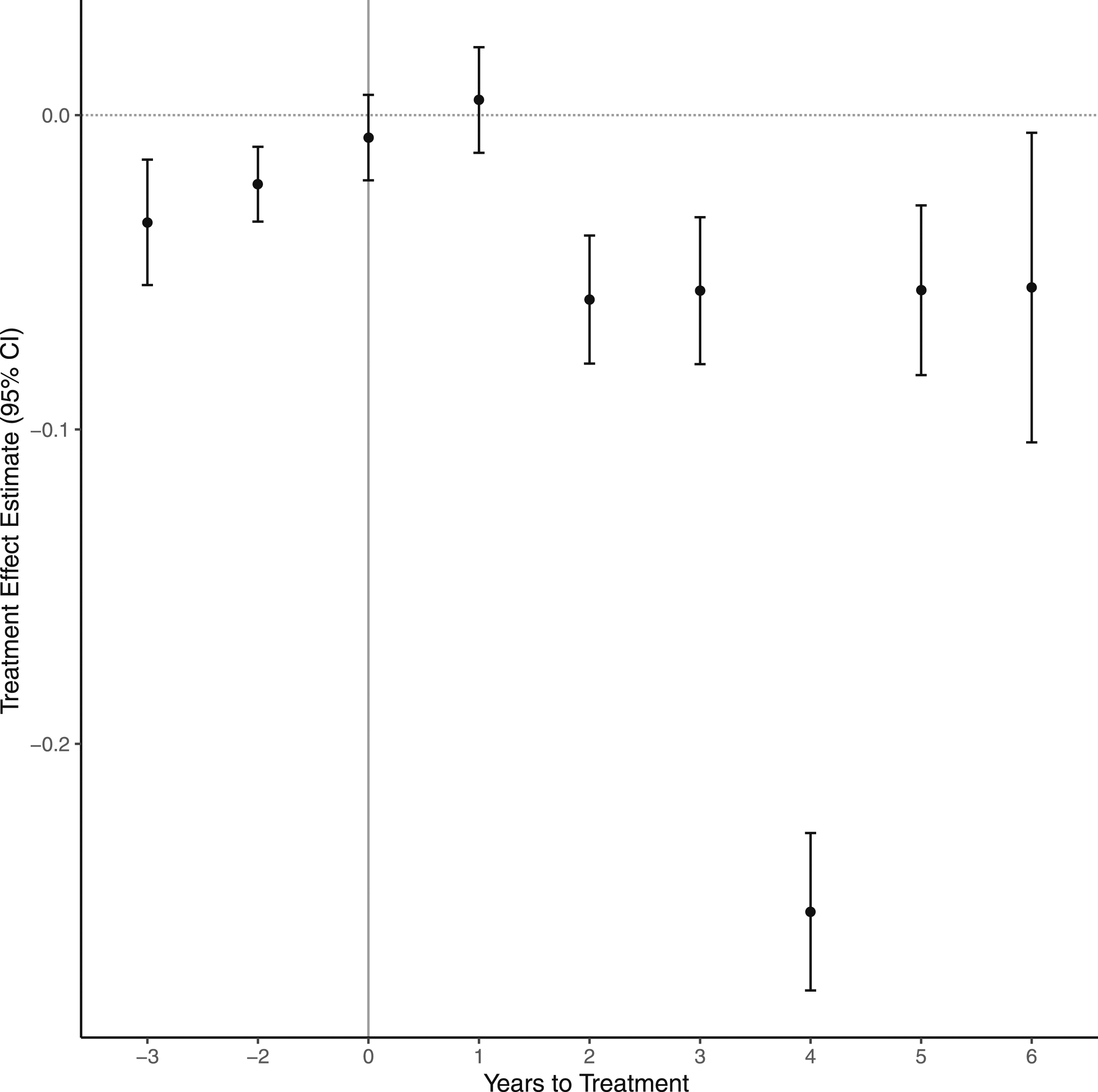

Appendix D. Comparing Tuition Rates Across Institutions in Washington State Over Time.

Table A1.

Tuition Rates Across Institutions in Washington State Over Time.

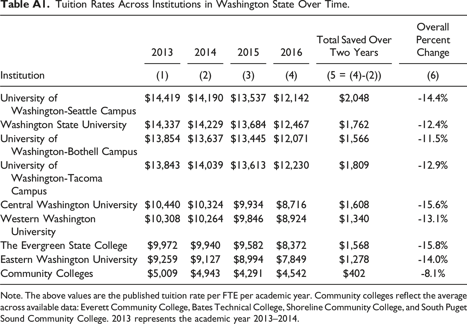
Institution	2013	2014	2015	2016	Total Saved Over Two Years	Overall Percent Change
Institution	(1)	(2)	(3)	(4)	(5 = (4)-(2))	(6)
University of Washington-Seattle Campus	$14,419	$14,190	$13,537	$12,142	$2,048	-14.4%
Washington State University	$14,337	$14,229	$13,684	$12,467	$1,762	-12.4%
University of Washington-Bothell Campus	$13,854	$13,637	$13,445	$12,071	$1,566	-11.5%
University of Washington-Tacoma Campus	$13,843	$14,039	$13,613	$12,230	$1,809	-12.9%
Central Washington University	$10,440	$10,324	$9,934	$8,716	$1,608	-15.6%
Western Washington University	$10,308	$10,264	$9,846	$8,924	$1,340	-13.1%
The Evergreen State College	$9,972	$9,940	$9,582	$8,372	$1,568	-15.8%
Eastern Washington University	$9,259	$9,127	$8,994	$7,849	$1,278	-14.0%
Community Colleges	$5,009	$4,943	$4,291	$4,542	$402	-8.1%

Note. The above values are the published tuition rate per FTE per academic year. Community colleges reflect the average across available data: Everett Community College, Bates Technical College, Shoreline Community College, and South Puget Sound Community College. 2013 represents the academic year 2013–2014.

Table A1 presents tuition rates for the eight treated universities and the average tuition across community colleges in Washington State for the 2013–14 to 2016–17 academic years. In Column 5, we compare tuition rates in the 2016–17 and 2014–15 academic years. This two-year difference in rates allows us to calculate the tuition savings due to the College Affordability Program.

Table A2.

Controlling for Changes in Unemployment.

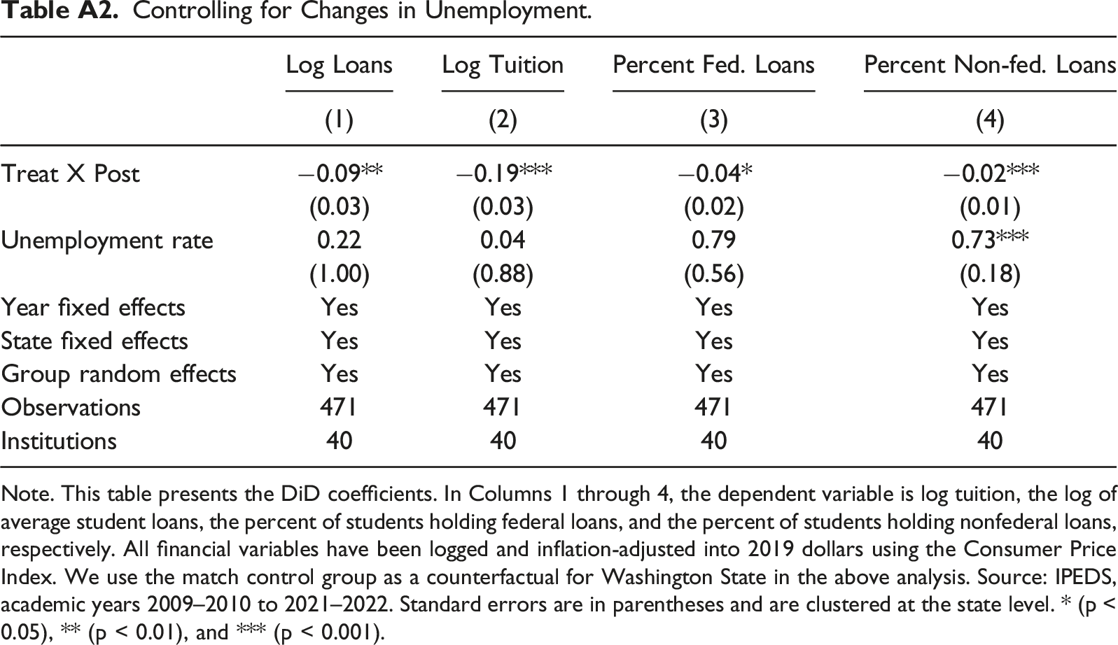
	Log Loans	Log Tuition	Percent Fed. Loans	Percent Non-fed. Loans
	(1)	(2)	(3)	(4)
Treat X Post	−0.09**	−0.19***	−0.04*	−0.02***
	(0.03)	(0.03)	(0.02)	(0.01)
Unemployment rate	0.22	0.04	0.79	0.73***
	(1.00)	(0.88)	(0.56)	(0.18)
Year fixed effects	Yes	Yes	Yes	Yes
State fixed effects	Yes	Yes	Yes	Yes
Group random effects	Yes	Yes	Yes	Yes
Observations	471	471	471	471
Institutions	40	40	40	40

Note. This table presents the DiD coefficients. In Columns 1 through 4, the dependent variable is log tuition, the log of average student loans, the percent of students holding federal loans, and the percent of students holding nonfederal loans, respectively. All financial variables have been logged and inflation-adjusted into 2019 dollars using the Consumer Price Index. We use the match control group as a counterfactual for Washington State in the above analysis. Source: IPEDS, academic years 2009–2010 to 2021–2022. Standard errors are in parentheses and are clustered at the state level. * (p < 0.05), ** (p < 0.01), and *** (p < 0.001).

Cross-validation is typically performed by removing a fixed number of random observations from the sample and re-estimating the model. However, due to the carefully crafted structure of the study, we opted to remove entire matched groups. Matched group cross-validation removes one treated college in Washington in addition to all of the matched control colleges. This method ensures that the treatment-to-control group ratio is fixed.

Figure A5 compares the average treatment effect estimates resulting from removing a single matched group against the overall matched sample estimate of -0.12 percentage points. Using 95% confidence interval bands, no matched group has a significantly different estimate compared to the overall average.

Figure A5.

Cross-validation using matched groups.

Author Biographies

Tennecia Dacass is an Assistant Professor in the Department of Economics at Central Washington University. Tennecia is an applied microeconomist specializing in labor and public economics.

Zachary Dowdy obtained his Bachelor of Science in Economics and Bachelor of Arts in Psychology from Central Washington University. His scholarly interests include the economics of labor and higher education.

References

Abel

J. R.

Deitz

(2019). The cost of college continues to climb (No. 20190603). Federal Reserve Bank of.

Baker

A. R.

Andrews

B. D.

McDaniel

(2017). The impact of student loans on college access, completion, and returns. Sociology Compass, 11(6), e12480. https://doi.org/10.1111/soc4.12480

Barr

Turner

(2015). Out of work and into school: Labor market policies and college enrollment during the Great Recession. Journal of Public Economics, 124, 63–73. https://doi.org/10.1016/j.jpubeco.2014.12.009.

Betts

J. R.

McFarland

L. L.

(1995). Safe port in a storm: The impact of labor market conditions on community college enrollments. Journal of Human Resources, 30(4), 741–765. https://doi.org/10.2307/146230

Bleemer

Brown

Lee

Strair

Van der Klaauw

(2021). Echoes of rising tuition in students’ borrowing, educational attainment, and homeownership in post-recession America. Journal of Urban Economics, 122(5), 103298. https://doi.org/10.1016/j.jue.2020.103298

Bozick

Estacion

(2014). Do student loans delay marriage? Debt repayment and family formation in young adulthood. Demographic Research, 30(1), 1865–1891. https://doi.org/10.4054/demres.2014.30.69

Cabral

Kim

Rossin-Slater

Schnell

Schwandt

(2021). Trauma at school: The impacts of shootings on students' human capital and economic outcomes (No. w28311). National Bureau of Economic Research.

Chakrabarti

Fos

Liberman

Yannelis

(2023). Tuition, debt, and human capital. The Review of Financial Studies, 36(4), 1667–1702. https://doi.org/10.1093/rfs/hhac065

Chen

(2008). Financial Aid and Student Dropout in Higher Education: A Heterogeneous Research Approach. In Smart

J. C.

(Ed.), Higher Education. Handbook of Theory and Research (23). Springer. https://doi.org/10.1007/978-1-4020-6959-8_7

10.

Daniels

G. E.

Jr Smythe

(2019, May). Student debt and labor market outcomes. In AEA Papers and Proceedings (Vol. 109, pp. 171–175), TN, USA, 2014. American Economic Association.

11.

Dunbar

Hossler

Shapiro

Chen

Martin

Torres

Ziskin

(2011). National postsecondary enrollment trends: Before, during, and after the Great recession. Signature [TM] report 1. National Student Clearinghouse.

12.

Dziak

J. J.

Dierker

L. C.

Abar

(2020). The interpretation of statistical power after the data have been gathered. Current Psychology, 39(3), 870–877. https://doi.org/10.1007/s12144-018-0018-1

13.

Federal Reserve Bank of New York . (2022). Household debt and credit report (Q1 2022). Tech. Rep. Center for microeconomic data. https://www.newyorkfed.org/medialibrary/interactives/householdcredit/data/pdf/hhdc_2022q1.pdf. (Accessed on:2022 07 12)

14.

Froidevaux

Koopmann

Wang

Bamberger

(2020). Is student loan debt good or bad for full-time employment upon graduation from college? Journal of Applied Psychology, 105(11), 1246–1261. https://doi.org/10.1037/apl0000487

15.

Gordon

Hedlund

(2016). Accounting for the rise in college tuition (No. w21967). National Bureau of Economic Research.

16.

Hillman

N. W.

Orians

E. L.

(2013). Community colleges and labor market conditions: How does enrollment demand change relative to local unemployment rates? Research in Higher Education, 54(7), 765–780. https://doi.org/10.1007/s11162-013-9294-7

17.

Hillman

N. W.

Tandberg

D. A.

Fryar

A. H.

(2015). Evaluating the impacts of “new” performance funding in higher education. Educational Evaluation and Policy Analysis, 37(4), 501–519. https://doi.org/10.3102/0162373714560224

18.

Imbens

G. W.

(2004). Nonparametric estimation of average treatment effects under exogeneity: A review. The Review of Economics and Statistics, 86(1), 4–29. https://doi.org/10.1162/003465304323023651

19.

IPEDS . (2021). U.S. Department of Education. National Center for Education Statistics. https://nces.ed.gov/ipeds/datacenter/InstitutionByName.aspx?_goToReportId=5. (Accessed on 07 12).

20.

Jackson

B. A.

Reynolds

J. R.

(2013). The price of opportunity: Race, student loan debt, and college achievement. Sociological Inquiry, 83(3), 335–368. https://doi.org/10.1111/soin.12012

21.

Kelchen

(2019). An empirical examination of the Bennett Hypothesis in law school prices. Economics of Education Review, 73(3), 101915. https://doi.org/10.1016/j.econedurev.2019.101915

22.

Lucca

D. O.

Nadauld

Shen

(2019). Credit supply and the rise in college tuition: Evidence from the expansion in federal student aid programs. The Review of Financial Studies, 32(2), 423–466. https://doi.org/10.1093/rfs/hhy069

23.

Macy

Terry

(2007). The determinants of student college debt. Southwestern Economic Review, 34, 15–25.

24.

Miller

(2017). Deeper in debt: Women and student loans. American Association of University Women.

25.

Mullin

C. M.

Phillippe

(2009). Community college enrollment surge: An analysis of estimated fall 2009 headcount enrollments at community colleges. Policy brief 2009-01PBL. American Association of Community Colleges. (NJ1).

26.

Odle

T. K.

Lee

J. C.

Gentile

S. P.

(2021). Do promise programs reduce student loans? Evidence from Tennessee promise. The Journal of Higher Education, 92(6), 847–876. https://doi.org/10.1080/00221546.2021.1888674

27.

Price

G. N.

Surprenant

C. W.

(2022). The treatment effect of business education on the supply of high school entrepreneurs in Atlanta and New Orleans. The American Economist, 67(1), 85–98. https://doi.org/10.1177/05694345211016310

28.

Robb

C. A.

Chatterjee

Porto

Cude

B. J.

(2019). The influence of student loan debt on financial satisfaction. Journal of Family and Economic Issues, 40(1), 51–73. https://doi.org/10.1007/s10834-018-9599-y

29.

Siripurapu

Speier

(2021). Is rising student debt harming the US economy. Foreign Affairs, 59(2), 174–197.

30.

Velez

Cominole

Bentz

(2019). Debt burden after college: The effect of student loan debt on graduates’ employment, additional schooling, family formation, and home ownership. Education Economics, 27(2), 186–206. https://doi.org/10.1080/09645292.2018.1541167

31.

Washington State Senate . (2015). Second Engrossed Substitute Senate Bill 5954, Chapter 36. https://lawfilesext.leg.wa.gov/biennium/2015-16/Pdf/Bills/Session_Laws/Senate/5954-S.SL.pdf [Accessed on: 2021-12-17].

Student Loan Debt Response to Tuition Changes

Abstract

Keywords

Introduction

Policy Background

Data

Variables

Methodology

Matching Procedure

Difference-in-Differences Framework

Event Study Model

Results

Trends in Outcomes

Regression Results

Robustness of Regression Results

Conclusion

Footnotes

Declaration of Conflicting Interests

Funding

ORCID iDs

Notes

Appendix A. Proportion of Revenue and Expenses from and on Higher Education.

Appendix B. Assessment of Balance after Matching.

Appendix C. Event Studies for Alternate Control Groups.

Appendix D. Comparing Tuition Rates Across Institutions in Washington State Over Time.

Author Biographies

References