
Abstract
Accurate destination choice modeling is vital for transportation and urban planning, influencing demand prediction, infrastructure development, and policy assessment. Conventional methods for choice set generation—both deterministic and stochastic—often face limitations such as failing to capture individual variability, requiring extensive data, and inadequately representing decision-making processes, thus compromising reliability. This study introduces a novel application of variational autoencoders (VAEs) for generating choice sets in destination choice modeling, focusing on home-based work trips in Montreal, Canada. Leveraging the deep generative capabilities of VAEs enhances the realism and diversity of choice sets, addressing implicit perception and availability of alternatives. Our methodology integrates VAE-generated choice sets with a multinomial logit model to predict destination choices. The results show significant improvements in model fit and predictive accuracy. The VAE-based model achieved a
Introduction
Destination choice modeling is an important component in transportation and urban planning, involving the prediction of individual location choice among numerous potential destinations. Accurate destination choice models are essential for applications such as demand prediction, infrastructure planning, and policy evaluation. The process typically comprises two main steps: choice set generation and the modeling of choices from the generated choice sets. These two steps are required because the actual set of alternatives considered by individuals before making a decision is generally unobservable and can vary significantly among individuals; therefore, any misspecification in the choice set can lead to biased and inconsistent parameter estimates, affecting the reliability of the model’s predictions ( 1 ).
The generation of choice sets poses several challenges. First, it is generally impossible to identify the exact alternatives an individual considers before making a decision. Moreover, when dealing with a vast number of potential alternatives, enumerating all feasible options becomes impractical ( 2 , 3 ). To address these issues, various choice set generation methods have been developed, which can generally be categorized into deterministic and stochastic approaches.
Deterministic methods involve predefined rules or criteria to generate choice sets. Common examples include rule-based methods where alternatives are included or excluded based on specific attributes or thresholds. For instance, a rule might exclude destinations beyond a certain travel time or distance. While straightforward, deterministic methods often oversimplify the decision-making process by excluding viable alternatives that do not meet rigid criteria, potentially leading to biased choice sets ( 4 ). Moreover, deterministic methods rely on predefined generation rules, leading to the generation of the same set of alternatives for a given observation each time. This contradicts the concept that the true consideration set can differ among individuals.
Stochastic methods incorporate randomness into the choice set generation process, utilizing techniques such as random sampling and importance sampling. These methods aim to represent the decision-making process more flexibly by allowing for variability in the choice sets generated for different individuals or scenarios. While stochastic methods are often computationally manageable in essence, their complexity can increase in practical applications, particularly when dealing with large datasets, numerous alternatives, or the need for repeated sampling and weighting adjustments ( 5 , 6 ). Additionally, in the context of large choice sets and the inherent difficulty of recognizing the true consideration set, these methods are often simplified to balance computational feasibility. For instance, Cascetta et al. generated choice sets by modeling the implicit availability or perception of alternatives using a simple binomial logit model ( 7 ).
The limitations with traditional methods necessitate a need for developing a more comprehensive modeling framework for choice set formation. It is also important to note that the concept of choice set generation is prevalent in other areas of transportation research, especially when dealing with many potential alternatives. A notable example is route choice modeling, where recent advancements have been particularly noteworthy. For instance, Yao and Bekhor combined machine learning (ML) with discrete choice models to generate choice sets with high prediction accuracy ( 8 ).
Similarly, deep generative methods such as generative adversarial networks (GANs) and variational autoencoders (VAEs) have demonstrated significant success in generating realistic high-dimensional data across various domains, including image synthesis and natural language processing ( 9 , 10 ). These models learn the underlying data distribution and use it to generate new realistic samples, making them highly suitable for applications requiring the generation of realistic alternatives. GANs function through an adversarial training framework, in which a generator produces synthetic samples aimed at deceiving a discriminator tasked with distinguishing between real and generated data. This mechanism enables GAN models to generate visually compelling and detailed synthetic samples. However, despite these strengths, GANs possess certain limitations that become particularly critical in choice set generation contexts. Most notably, GANs do not provide an explicit probabilistic model of data, as they do not inherently estimate data likelihood. Instead, they rely entirely on adversarial competition, which can lead to unstable training, mode collapse (limited diversity among generated samples), and convergence issues ( 11 ). Additionally, in the context of choice set generation, the actual consideration sets of individuals are typically unknown, meaning there is no clearly defined “real” dataset to effectively implement the adversarial framework.
In contrast, VAEs stand out as particularly well-suited for choice set generation because of several key attributes. VAEs are typically self-supervised; their performance is directly evaluated by comparing regenerated samples against the original input data. This characteristic is particularly beneficial in scenarios involving unlabeled datasets, as is the case in choice set generation. Given the typically unknown true consideration sets, the VAE framework provides a flexible means of estimating the likelihood that an alternative belongs within an individual’s implicit consideration set. Furthermore, VAEs explicitly infer structured latent representations from observed samples. This explicit probabilistic modeling enables meaningful interpretation of latent factors underlying decision-making processes. Together, these features make VAEs especially appropriate and effective for generating realistic and behaviorally meaningful choice sets. In the context of route choice modeling, Yao and Bekhor proposed a VAE-based approach that considers the implicit perception and availability of alternatives ( 12 ). Their method maximizes the likelihood of including chosen alternatives in the generated choice set by modeling the underlying generation process. Their study demonstrated that the VAE method could effectively reproduce true values and outperform traditional methods in goodness-of-fit and predictive performance.
The potential of VAEs in choice set generation, extends beyond route choice modeling, as the underlying principles of choice set generation and perception of alternatives are applicable to other similar domains such as destination choice modeling. However, as far as we know, these deep generative models, especially VAE, have not yet been adapted for choice set generation in destination choice modeling. By leveraging the VAE approach, we can enhance the generation of destination choice sets, accounting for the implicit perception of alternatives and improving the robustness of destination choice models.
In this paper, we draw inspiration from the VAE-based choice set generation method proposed by Yao and Bekhor and adapt its principles to the context of choice set generation in destination choice modeling ( 12 ). We compute the implicit perception and availability of alternatives from these generated sets and implement them in a multinomial logit (MNL) model to predict the destination choices of home-based work trips, using a case study in Montreal, Canada.
This study makes two key contribution. First, we address the challenges of large and unobservable true choice sets in destination choice modeling by using a VAE to generate choice sets. Secondly, we provide a comprehensive evaluation of the VAE approach using the Montreal Origin-Destination (OD) Survey dataset, demonstrating its applicability and effectiveness in real-world scenarios ( 36 ).
The rest of the paper is structured as follows. The Literature Review discusses previous methods of choice set generation, while the Methodology section details the VAE method used in this paper for choice set generation. The Data section details the dataset used in the study and the attributes incorporated into the models. The Results and Discussion section presents the findings, and the Conclusion summarizes the key insights and implications of the study.
Literature Review
Choice set formation is a critical step in the specification, estimation, and application of destination choice models. As noted by Thill, misspecification of choice sets can adversely affect parameter estimates and the accuracy of predicted choice probabilities ( 13 ). Accurate definition of the destination choice set is essential because the number of potential alternatives can be extremely large, especially in urban contexts where hundreds of zones are involved. This section provides a detailed review of traditional and advanced methods for choice set generation in discrete choice modeling, with traditional methods broadly categorized into deterministic and stochastic approaches.
Deterministic Methods
Deterministic methods, such as those used by Scott and He, and Ben-Akiva and Lerman, rely on predefined rules to generate alternatives ( 14 , 15 ). These methods, while systematic and straightforward, often fail to capture the variability in individual preferences and can result in overly simplistic choice sets. For example, Bhat et al. employed a deterministic approach to model destination choice for work and shopping trips in Boston, using the generalized cost (time and monetary) as a key determinant in generating choice sets ( 16 ). This method categorized alternatives based on fixed criteria, failing to account for individual preferences that might lead to more diverse or unconventional choices. Bowman and Ben-Akiva applied deterministic rules in an activity-based travel demand model, focusing on factors such as time, distance, and monetary cost to generate choice sets ( 17 ). Although clear and simple, this method often led to the exclusion of feasible alternatives that did not meet predetermined criteria, such as destinations offering unique amenities or opportunities outside predefined bounds. Sivakumar and Bhat used a generalized cost approach, including both time and monetary aspects, to generate choice sets for non-work trips ( 18 ). Despite detailed cost considerations, this deterministic method excluded relevant alternatives because of rigid predefined criteria. Finally, the time-space prism approach, based on time geography, maps activity spaces where individuals travel and engage in activities ( 19 ). While providing a more dynamic and flexible representation of travel behavior than other deterministic methods, it still imposes deterministic constraints that can overlook viable alternatives. These limitations highlight the failure of deterministic methods to account for variability in individual preferences, often resulting in the exclusion significant alternatives.
Stochastic Methods
Stochastic methods introduce randomness to capture variability in decision-making processes. For example, Pel et al. used random utility models to generate choice sets, integrating randomness to better reflect real-world decision-making processes ( 20 ). Molloy used a zonal-based approach that incorporated randomness by considering different zones for destination choices in Ontario ( 21 ). This method captured spatial variability but required extensive data on zone characteristics and boundaries. Additionally, Tsoleridis et al. proposed a probabilistic approach to choice set formation by integrating the concept of activity spaces in mode and destination choice modeling ( 22 ). This approach involves inherent randomness in representing individuals’ habitual activity spaces. Similarly, Elgar et al. introduced the concept of anchor points in modeling the location decisions of office firms ( 23 ). Their method involves creating choice sets that reflect the spatial structure and constraints faced by firms through the introduction of random anchor points.
In addition, sampling methods are frequently used to generate choice sets by incorporating randomness. Two commonly employed sampling approaches are random sampling and importance sampling. In random sampling approaches, a random sample of locations is drawn from the universe of feasible choices to constitute the consideration choice set. Each alternative in the universe of feasible choices has an equal probability of being selected. This method is straightforward and ensures that all potential choices have an equal chance of inclusion, which can provide a broad representation of possible alternatives. In contrast, in importance sampling approaches, some destinations are considered more desirable based on variables like size and distance. Monte Carlo simulations sample destinations from an importance probability distribution, requiring correction factors to maintain the properties of the maximum likelihood estimator.
Stochastic methods that incorporate these sampling techniques have been extensively applied in transportation and urban planning research. Jonnalagadda et al. employed a combination of stratification by importance and random sampling to generate choice sets for work and intermediate trips in San Francisco ( 24 ). This method introduced variability while still relying heavily on initial stratification criteria. Pozsgay and Bhat implemented a simple random method to generate choice sets for leisure trips in Dallas-Fort Worth ( 25 ). While this approach allowed for a broader range of alternatives, it also increased the potential inclusion of irrelevant options. Similarly, Kim et al. and Mishra et al. applied random sampling techniques in their comparative studies of aggregate and disaggregate models, aiming to include a diverse range of alternatives but often struggling with ensuring adequate representation of all relevant alternatives ( 26 , 27 ). Hammadou et al. used a spatial analysis approach with random sampling in Antwerp, emphasizing the importance of spatial dimensions in choice set generation ( 28 ). While this method enhanced the spatial realism of choice sets, it faced challenges in ensuring the relevance of included alternatives. Li et al. applied geographically stratified importance sampling for destination choice modeling in Maryland ( 29 ). Consistent with this, Shiftan used a stratified-by-importance method for generating choice sets in trip chaining models ( 30 ). This approach categorized alternatives by importance but often neglected less obvious yet significant alternatives, such as destinations that individuals might consider because of unique preferences or specific constraints. To elucidate this further, consider a situation where individuals, in the context of work destination choices, may select jobs in faraway locations because of limited local job opportunities or the need for specialized employment. Thus, although stochastic methods introduce flexibility, they tend to oversimplify the choice set formation process and struggle to fully reflect the actual consideration set of individuals.
Recent Advances in Choice Set Generation
As mentioned before, recent advances in choice set generation using ML and deep learning (DL) algorithms have been primarily applied in route choice models. Because of the similarities between route choice models and destination choice models, particularly in handling many alternatives, these advanced methods hold significant potential for application in choice set generation for destination choice models.
In this regard, Yao and Bekhor proposed a novel data-driven framework for choice set generation in route choice modeling by combining ML techniques with observed route data ( 8 ). Their method utilized clustering and classification to detect patterns in travelers’ revealed preferences, enabling the generation of personalized and behaviorally realistic choice sets without relying on arbitrary rules. This method demonstrated high prediction accuracy and strong explanatory power compared with conventional methods. Another innovative approach is the “Neural Choice by Elimination” framework introduced by Tran et al. ( 31 ). This framework integrates DL into probabilistic sequential choice models and proved competitive against state-of-the-art learning to rank methods.
VAEs have been used for choice set generation in route choice modeling. Yao and Bekhor proposed using VAEs to generate choice sets by maximizing the likelihood of including chosen alternatives ( 12 ). This method effectively bridges ML methods with traditional choice models by incorporating implicit availability and perception of alternatives. Liu et al. proposed a hybrid choice set generation approach for route choice modeling using a conditional VEA ( 32 ). Their method built on the earlier VAE framework by Yao and Bekhor and incorporates individual- and OD-specific features as conditioning variables, allowing the model to generate alternatives that are more personalized and context-specific ( 12 ).
In summary, traditional choice set generation methods, whether deterministic or stochastic, face limitations that can affect their practicality and accuracy. Deterministic methods often exclude feasible alternatives because of strict criteria, while stochastic methods, despite their flexibility, may still struggle with retrieving the true consideration set and rely on simplified representations of the decision-making process. Both approaches have inherent challenges that can affect the reliability of destination choice models. Recent advancements in using ML methods for choice set generation highlight the potential of these techniques to enhance the predictive power and reliability of choice models. Despite these advancements, there remains a significant gap in evaluating the adoption of such advanced methods for choice set generation in destination choice modeling. Given the features of VAEs, such as their self-supervised nature which is advantageous for handling unlabeled data, and their strength in learning the latent distribution of observed samples, along with promising results in previous studies, this paper implements a VAE approach to generate choice sets in destination choice modeling. Our findings demonstrate the effectiveness of this approach in this new context.
Methodology
The methodology for choice set generation in destination choice modeling consists of three main components: choice set generation using VAEs, computing the implicit availability/perception of alternatives, and the discrete choice model for destination choice prediction. This section closely follows Yao and Bekhor and we refer interested readers to their paper for further discussions and in-depth explanations of the mathematical foundations ( 12 ).
Choice Set Generation Using VAE
The VAE model architecture comprises an encoder and a decoder. The encoder maps observed alternatives to a lower-dimensional latent space capturing the essential features of the alternatives. The decoder reconstructs the alternatives from the latent space, generating new samples consistent with the observed data.
The encoder

where
The decoder

where
I = the identity matrix.
The VAE model aims to maximize the likelihood of including chosen alternatives in the generated choice set by learning the underlying distribution of the alternatives. The underlying distribution learned by the VAE represents the distance distribution of chosen trip destinations across census tracts in the study area. Specifically, it captures the normalized distance between origin and destination zones as the primary attribute. This focus on distance ensures the generated alternatives reflect realistic spatial patterns observed in the data and aligns with its critical role in destination choice modeling. While the VAE framework is capable of incorporating multiple distributions, such as population density, total residents, and trip density, this study focuses on distance as a foundational attribute for model evaluation. Including additional distributions in the latent space would enhance the richness of generated choice sets and is an important direction for future work.
The objective function, specifically formulated in this paper for training the VAE, includes three main components: the reconstruction loss, the Kullback-Leibler (KL) divergence, and the total correlation regularizer. This combination helps in learning a compact representation of the data while promoting independence among the latent variables. The objective function is expressed as:
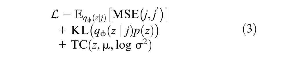
where
The reconstruction loss (mean squared error) measures how well the model reconstructs the input data, ensuring that the generated alternatives are close to the original ones ( 10 ). The KL divergence ensures that the learned latent space follows a standard normal distribution, promoting smoothness and enabling meaningful sampling ( 10 ). The total correlation term further encourages independence among the latent variables, reducing redundancy and improving the quality of the latent representations ( 33 ). This objective function is optimized using stochastic gradient descent with the Adam optimizer ( 34 ). The parameters of the encoder and decoder networks are updated to minimize this loss, effectively learning the distribution of the alternatives and enabling the generation of realistic and diverse choice sets. The model is trained by drawing multiple samples from the approximate posterior distribution and using these samples to calculate the expected reconstruction loss and regularization terms.
The training procedure for the VAE involves several key steps. First, the attributes of the observed alternatives are normalized to ensure consistent scaling across features. Next, the encoder maps the preprocessed input data into a lower-dimensional latent space, capturing the underlying structure of the alternatives in relation to compact latent variables. Once these latent representations are learned, the decoder reconstructs new alternatives by sampling from this latent space, generating alternatives that follow the same underlying distribution as the observed data. Finally, the model optimizes an importance-weighted log-likelihood objective, ensuring that the reconstructed and generated alternatives remain statistically consistent with the patterns observed in the original dataset.
Implicit Perception of Alternatives
In choice modeling contexts, individuals typically do not explicitly reveal all alternatives they consider; instead, some alternatives are implicitly perceived or considered within their choice sets without direct indication. We define the implicit availability/perception of alternatives as the likelihood that an alternative is implicitly included within an individual’s choice set, even though such perception is not directly observable or explicitly stated. This approach assumes that each alternative has an implicit degree of availability or perception represented as a probability. To quantify these implicit perception probabilities, we use the Bayesian conditional (BC) metric (
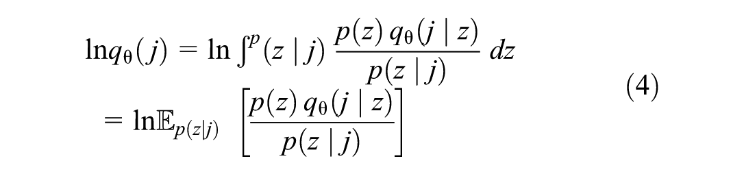
where
Because of the intractable nature of the posterior distribution
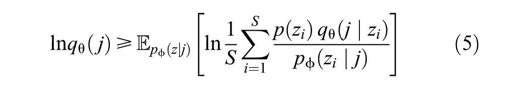
Consequently, the
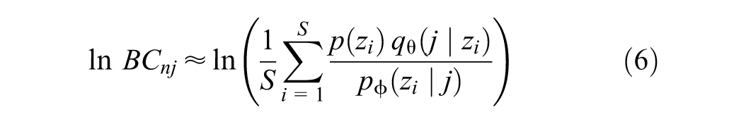
Further theoretical details and broader context are comprehensively discussed by Yao and Bekhor ( 12 ). The process of choice set generation and implicit perception estimation is summarized as follows.
Alternative Generation Steps
Draw
Draw a new alternative
Implicit Perception Estimation Steps
Draw
Draw from the decoder
Draw from prior distribution
Compute
Repeat steps 1–4 for
Calculate
To validate the generated choice sets, we adopted a two-step approach. First, we compared the distribution of generated alternatives with the distribution of chosen alternatives in the dataset. This comparison involved visual methods, such as density plots, and statistical measures. These methods were employed to assess how well the generated choice sets represent observed behavior.
In the second step of validation, the generated alternatives were used to create choice sets for individuals, incorporating the
To provide robust benchmarks, we included two traditional methods for choice set generation: simple random sampling and importance sampling. Simple random sampling serves as a baseline, where alternatives are selected purely at random, without any behavioral considerations. The importance sampling method was implemented following a gravity-based framework introduced by Ben-Akiva and Lerman (
1
). In this framework, the probability of selecting a destination zone is proportional to its size and inversely proportional to its distance from the traveler’s origin. This ensures that larger and closer zones are more likely to be included in the choice set, reflecting the behavioral tendency of travelers to prefer nearby, attractive destinations. The probability of choosing a destination zone

where
The implementation of importance sampling involves several steps. First, a size measure, such as population density or area, is assigned to each destination zone. When specific size data is unavailable, zones are assumed to have equal size, making distance the primary determinant of selection probability. The distance decay parameter
Discrete Choice Model for Destination Prediction
We employ an MNL model for destination choice prediction. The utility function

where
The probability of choosing alternative

Figure 1 illustrates the methodology employed in this paper for choice set generation and destination choice modeling using a VAE. The process starts with data preprocessing to normalize the data. The VAE generates choice sets through an encoder, which compresses input data into latent variables, and a decoder, which reconstructs the data. The encoder consists of two hidden layers producing mean (
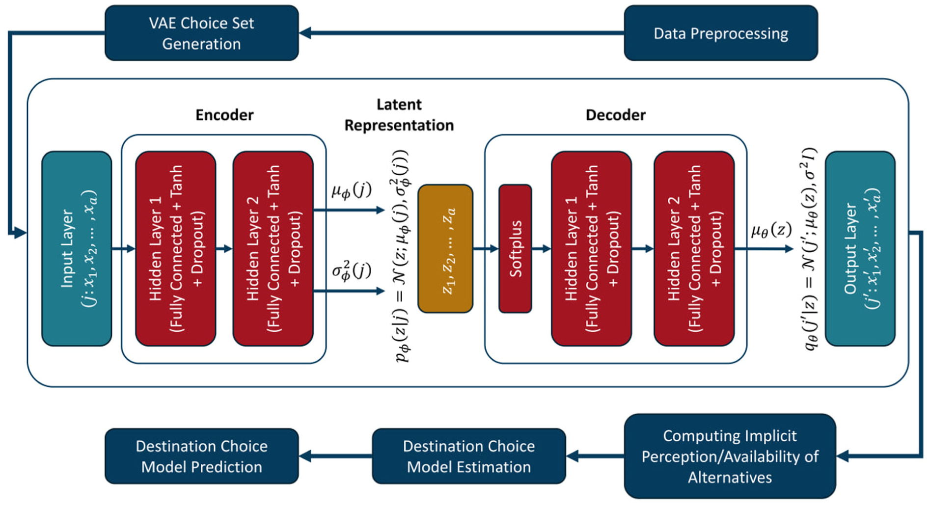
Process of implementing the suggested variational autoencoder (VAE) approach in destination choice modeling.
Study Area and Data
The primary focus of this study is the Island of Montreal, a part of the Greater Montreal metropolitan area. The study area covers a population of approximately 1.9 million people over an area of 462 square kilometers.
The dataset used in this study originates from the Enquête Origine-Destination 2018 survey which has been conducted every 5 years since 1970 ( 36 ). For the first time in 2018, the survey included an online questionnaire alongside traditional telephone interviews. This survey targeted weekday travel behavior and involved approximately 70,000 households, representing nearly 170,000 individuals and accounting for 393,826 trips. Participants in the OD survey were randomly selected and asked detailed questions about their household characteristics, individual demographics, and travel behaviors, capturing all trips made by each household member on the day before the interview.
The OD data covered the Greater Montreal area, but in this study, we filtered our data and focused on the Island of Montreal, as most trip destinations were located within this area. Moreover, the data were filtered to focus specifically on home-based work trips. Individuals under 16 years old and trips with unreasonable travel times (exceeding 3 hours or having zero travel time) were excluded from the analysis. The final database comprised 19,389 observations, representing 4.92% of the total dataset. Figure 2 shows the density distribution of each zone selected as a destination in the study area.
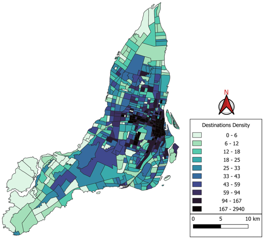
Density (per square kilometer) distribution of each zone selected as a destination in the study area.
Census tract data further enriched the dataset, providing additional attributes such as population, number of dwellings, employment rate, density, and the number of occupations in different categories. The study area was divided into 533 census tract zones, forming the basis for analyzing travel patterns and modeling destination choices in the Island of Montreal. Figure 3 illustrates the distribution of total number of all kinds of residents’ occupations across census tracts and the distribution of population density per square kilometer in each census tract of the study area.
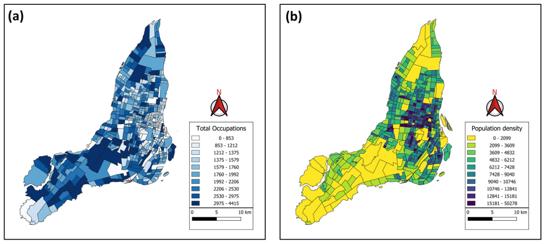
Distribution of: (a) total number of residents occupations (all categories) by census tract, and (b) population density (per square kilometer) by census tract in the Island of Montreal.
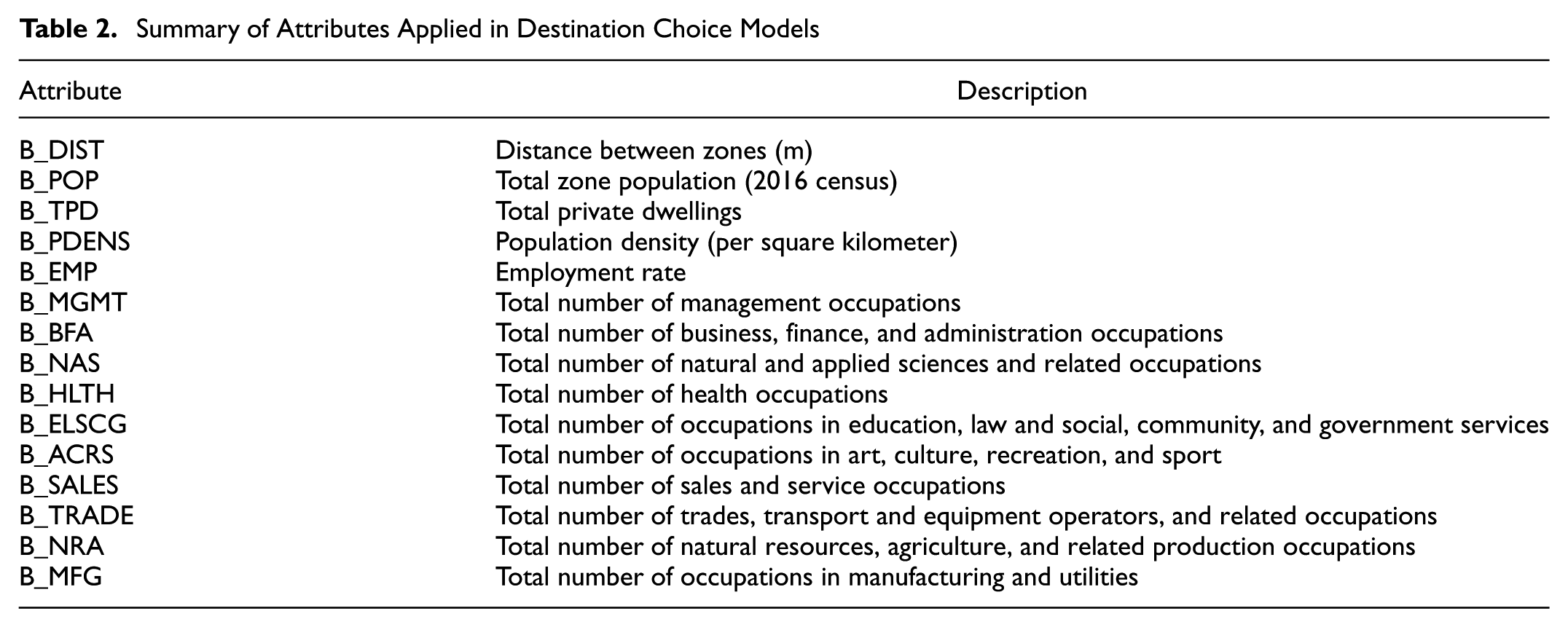
Travel time and distance were initially considered as impedance measures for each trip between the zone centroids. However, because of a high correlation between distance and travel time, the models were estimated using only the distance attribute. Table 1 provides summary statistics of the data and Table 2 details the attributes used in the estimated destination choice models.
Summary Statistics of the Data Features
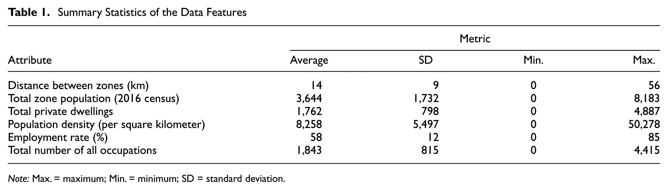
Note: Max. = maximum; Min. = minimum; SD = standard deviation.
Summary of Attributes Applied in Destination Choice Models
Results and Discussion
To train the VAE, a vector of normalized distances between the origin and all destinations is used as the attributes for each chosen alternative. The VAE is then trained to learn the distribution of chosen alternatives. Based on this distribution, 30 new alternatives are generated for each observation, resulting in a total of 581,670 generated alternatives (30 alternatives per observation multiplied by 19,389 observations). The BC term for these generated alternatives is calculated and incorporated into Equation 8 to predict destination choices. We normalized the input data using MinMaxScaler and used the Tanh activation function in hidden layers of both the encoder and decoder. Batch normalization and a dropout rate of 0.5 were applied to improve training stability and prevent overfitting. Weights were initialized using He initialization ( 37 ). The latent space dimension was set to 20 with hidden layers containing 128 neurons each. The encoder consists of two hidden layers, while the decoder has an additional Softplus layer to ensure that the generated values are not negative, as the input values represent distances and cannot be negative. To determine the optimal configuration, we tested a range of hyperparameters, as shown in Table 3. The final chosen values are underlined in the table.
Specifications of Neural Network Variational Autoencoder Model
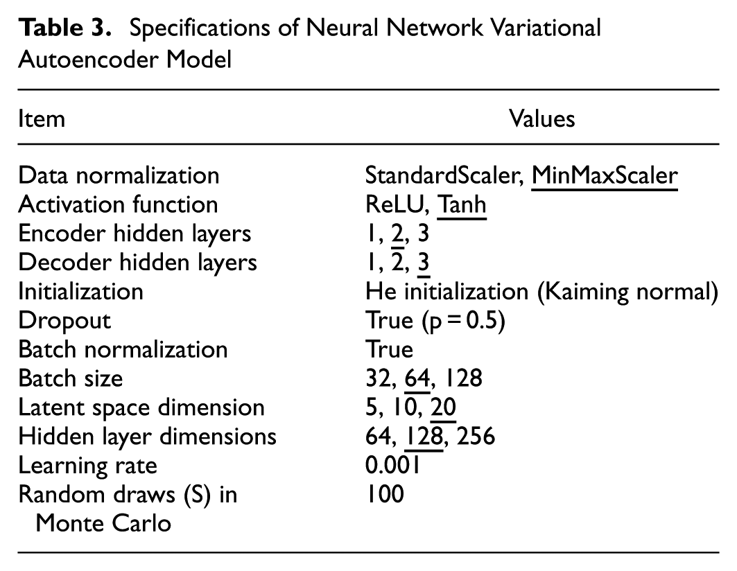
The primary criteria for evaluating each hyperparameter combination were the alignment of the generated alternatives’ distribution with the chosen alternatives’ distribution and the final log-likelihood of the destination choice model. We visually and statistically compared the density plots of generated and chosen alternatives to assess how well the VAE model captured the underlying data distribution, and we used higher log-likelihood values to indicate better performance in capturing the observed data. Based on these evaluation criteria, we selected the hyperparameters that resulted in the generated alternatives having a distribution most similar to that of the chosen alternatives and achieved the highest log-likelihood in the destination choice model.
Alternative Generation Using VAE
To analyze the performance of generated attributes of alternatives by the VAE in recognizing the distribution of the chosen alternatives, we used a KDTree algorithm for efficient nearest neighbor search ( 38 ). This method involves constructing a KDTree using the scaled values from the original dataset and identifying the closest destination for each generated alternative by querying the KDTree. Parallel processing is used to expedite the mapping process, ensuring efficiency and speed.
Evaluating the quality of generated choice sets is inherently challenging because of the unobservable nature of true consideration sets. In our study, we compared the distribution of chosen alternatives from the survey with the distribution of alternatives generated by VAE. While this is not a common approach in the literature, traditional deterministic and stochastic methods do not explicitly aim to capture the underlying distribution of consideration sets. By contrast, the VAE approach seeks to approximate the true distribution of individuals’ consideration sets, making this comparison a meaningful way to evaluate its performance.
The plot shown in Figure 4 presents the comparison between the density of chosen alternatives and generated alternatives by VAE across all zones. The chosen alternatives show specific patterns and the alignment of peaks and variations in the density of generated alternatives with those of the chosen alternatives suggests that the VAE model accurately learns the underlying data distribution, enabling it to generate plausible and diverse alternatives. However, the trained VAE model tends to produce higher density peaks in certain zones, particularly noticeable at the first peak. This happens because the model might generate alternatives biased toward regions with higher prior probabilities when sampling from the latent space, causing the generated density to be more concentrated around popular zones. This bias could actually be beneficial for the choice set generation case, as zones with higher probabilities of being chosen are more represented in the choice sets. Further validation of the quality of generated choices will be discussed in the estimation results of the destination choice model with these generated choices by VAE. Also, to quantitatively assess the similarity between these distributions, we employed two metrics: the histogram intersection index and the Jensen-Shannon (JS) divergence. The histogram intersection index, introduced by Swain and Ballard, measures the overlap between the density distributions of the chosen and generated alternatives ( 39 ). It yielded a score of 0.8634, indicating that 86.34% of the total area under the density curves of the chosen and generated alternatives overlaps. This high score suggests that the VAE model has effectively captured the overall pattern of the chosen alternatives’ distribution.
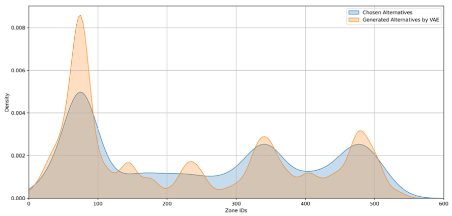
Density plot of chosen and generated alternatives.
The JS divergence, as introduced by Lin, is a symmetric measure of divergence between two probability distributions, providing an additional perspective on the similarity between the distributions ( 40 ). It produced a value of 0.1402, where lower values (bounded between 0 and 1) indicate greater similarity. This relatively low divergence further confirms that the generated alternatives closely mimic the chosen alternatives in distributional characteristics.
Further validation is provided by the cumulative distribution functions (CDFs) of chosen and generated alternatives in Figure 5. The VAE-generated alternatives exhibit a cumulative distribution that closely follows the trajectory of the chosen alternatives’ CDF, further validating the effectiveness of the VAE model in replicating the observed choice behavior.
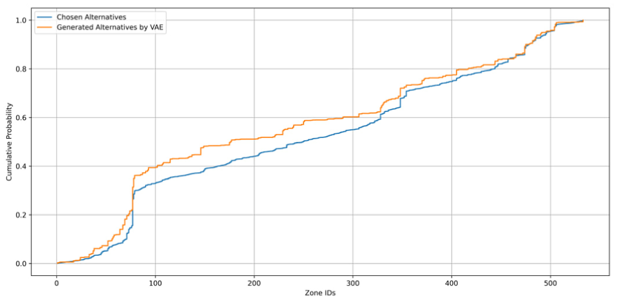
Cumulative distribution functions of chosen and generated alternatives.
To provide additional support for the behavioral realism of choice sets generated by different methods, we analyzed how frequently each generated set included the actual chosen destination. Figure 6 provides a visual comparison among the VAE-based method, importance sampling, and simple random sampling, each generating sets of 30 alternatives per individual. As depicted in Figure 6, the VAE-generated choice sets included the actual chosen alternatives in approximately 25.15% of cases, significantly outperforming importance sampling (7.66%) and simple random sampling (5.59%). These results provide additional support that the VAE approach generates choice sets that more closely reflect observed decision-making behavior.
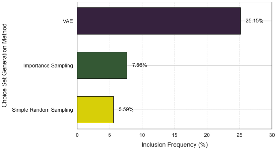
Inclusion frequency of chosen alternatives by choice set generation method.
Model Estimates
The model estimates for the destination choice models provide a comparative analysis of the performance of four different models: the destination choice model with all alternatives available (DC-FA), the destination choice model with choice sets generated by a simple random sample method (DC-SRS), the destination choice model with choice sets generated by importance sampling (DC-IS), and the destination choice model with choice sets generated by VAE (DC-VAE). All these models follow the MNL framework.
Validation is essential to prevent overfitting, where the model fits the estimation dataset well but performs poorly on other datasets. The validation process involves estimating the model with a subset of the total dataset, then applying the estimated parameters to the remaining validation subset. Accuracy is used as a performance measure. In this study, 80% of the database (15,517 out of 19,389 observations) is used for estimation and 20% (3,872 out of 19,389 observations) for validation. The percentage match rate between estimated and observed individual choices is analyzed as a performance metric. Performance measures are detailed in Table 4, including final log-likelihood,
Goodness-of-Fit and Prediction Performance Results
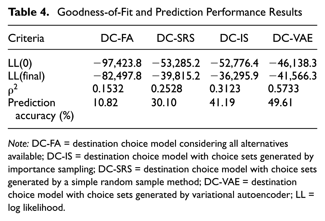
Note: DC-FA = destination choice model considering all alternatives available; DC-IS = destination choice model with choice sets generated by importance sampling; DC-SRS = destination choice model with choice sets generated by a simple random sample method; DC-VAE = destination choice model with choice sets generated by variational autoencoder; LL = log likelihood.
The goodness-of-fit and prediction performance metrics provide a comparative evaluation of the destination choice models. While DC-IS achieves the best (least negative) final log-likelihood at −36,295.9, followed by DC-VAE at −41,566.3, DC-SRS at −39,815.2, and DC-FA at −82,497.8, final log-likelihood alone does not fully capture overall model performance. Each model’s strengths must also be assessed in relation to their explanatory power and predictive accuracy, where clear differences are observed.
The
Prediction accuracy index measures the percent of correct predictions which highlights further distinctions between the models. DC-VAE achieves the highest accuracy at 49.61%, followed by 41.19% for DC-IS, 30.10% for DC-SRS, and 10.82% for DC-FA. The improved accuracy of DC-VAE underscores its ability to generate realistic choice sets that closely align with observed behavior, thereby enhancing predictive performance. DC-IS also demonstrates strong predictive accuracy compared with DC-SRS and DC-FA, confirming the effectiveness of probabilistic approaches such as importance sampling in creating behaviorally consistent choice sets.
To investigate the practicality and scalability of the proposed VAE method in large-scale applications, we compared the computational complexity and resource consumption across the different choice set generation methods (DC-FA, DC-SRS, DC-IS, and DC-VAE) and subsequent discrete choice model estimations. All experiments were executed on a system with an Intel Core i7 14700K CPU, 32 GB of RAM, and Nvidia RTX 4000 Ada GPU. The VAE model was implemented using PyTorch, while discrete choice models were estimated using the Apollo package (version 0.3.2) ( 43 ). The computational times for each method are summarized in Table 5.
Computational Times for Different Methods
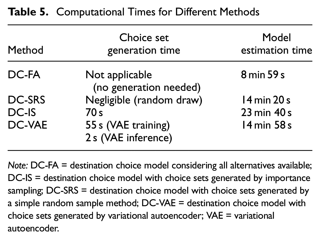
Note: DC-FA = destination choice model considering all alternatives available; DC-IS = destination choice model with choice sets generated by importance sampling; DC-SRS = destination choice model with choice sets generated by a simple random sample method; DC-VAE = destination choice model with choice sets generated by variational autoencoder; VAE = variational autoencoder.
The VAE approach has an initial non-trivial computational overhead associated with training (approximately 55 s for 100 epochs), but the training is a one-time investment. After training, the VAE’s inference phase for generating choice sets is extremely efficient, requiring only about 2 s, which is significantly faster than the importance sampling method (70 s). Although the simple random sampling (DC-SRS) method involves negligible computational effort because of its straightforward random draw process, it performs considerably worse in predictive accuracy than the VAE-based approach. Furthermore, while the DC-IS method offers improved predictive accuracy over DC-SRS, it still requires substantially longer inference times and exhibits some behavioral inconsistencies in its parameter estimations. In contrast, the DC-VAE method strikes a balance: after its initial training period, it achieves excellent inference-time efficiency combined with superior predictive performance.
The parameter estimates for the destination choice models are presented in Table 6. The results indicate that all parameter estimates are statistically significant at the 5% level, as evidenced by t-test values exceeding the critical threshold of 1.96. Across most models, the coefficient for distance (B_DIST) is negative, aligning with the well-established behavioral principle that individuals prefer closer destinations, typically characterized by a negative exponential relationship between distance and destination utility. This negative exponential form represents the diminishing likelihood of selecting a destination as its distance increases, reflecting realistic travel cost minimization and distance decay effects. However, the positive B_DIST coefficient in DC-IS contradicts this expectation and suggests a deeper examination. In the importance sampling approach, alternatives closer to the origin are disproportionately oversampled in the choice set. This results in a choice set where the actual chosen destination often has a longer distance than the majority of sampled alternatives. When the model estimates the likelihood of choosing a destination, it finds that longer distances are systematically associated with chosen alternatives relative to the sampled set, leading to an artificially positive relationship between distance and destination selection. This is a methodological artifact rather than a genuine behavioral preference. Our findings underline that the importance sampling approach, while offering improved predictive performance compared with simpler sampling methods such as random sampling, inherently carries significant methodological bias. Therefore, using importance sampling naively in choice set generation can lead to unrealistic behavioral interpretations and compromised parameter validity.
Parameter Estimation Results
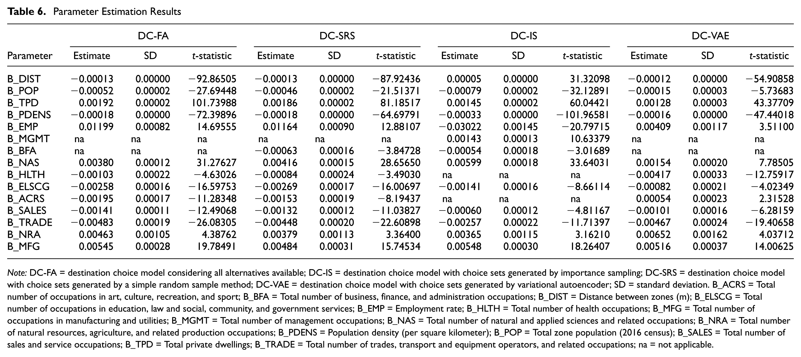
Note: DC-FA = destination choice model considering all alternatives available; DC-IS = destination choice model with choice sets generated by importance sampling; DC-SRS = destination choice model with choice sets generated by a simple random sample method; DC-VAE = destination choice model with choice sets generated by variational autoencoder; SD = standard deviation. B_ACRS = Total number of occupations in art, culture, recreation, and sport; B_BFA = Total number of business, finance, and administration occupations; B_DIST = Distance between zones (m); B_ELSCG = Total number of occupations in education, law and social, community, and government services; B_EMP = Employment rate; B_HLTH = Total number of health occupations; B_MFG = Total number of occupations in manufacturing and utilities; B_MGMT = Total number of management occupations; B_NAS = Total number of natural and applied sciences and related occupations; B_NRA = Total number of natural resources, agriculture, and related production occupations; B_PDENS = Population density (per square kilometer); B_POP = Total zone population (2016 census); B_SALES = Total number of sales and service occupations; B_TPD = Total private dwellings; B_TRADE = Total number of trades, transport and equipment operators, and related occupations; na = not applicable.
In continuation, the negative coefficient for total zone population (B_POP) across all models suggests that zones with higher populations are less likely to be chosen. This effect is strongest in the DC-IS model and weakest in the VAE-based model, reflecting variations in how these models account for population effects. For total private dwellings (B_TPD), the positive coefficient demonstrates that zones with more dwellings are more likely to be chosen, with the strongest effect observed in the DC-FA and DC-SRS models, followed by DC-IS, while the VAE-based model shows a more modest effect. The negative coefficient for population density (B_PDENS) suggests that higher density zones are less attractive as destinations, with the effect being most pronounced in the DC-IS model and least in the VAE-based model. The coefficient for employment (B_EMP) is positive in most models, indicating that zones with higher employment are generally more attractive. However, the DC-IS model shows a negative coefficient, which could suggest complex interactions within the choice set generated through importance sampling. Employment-related attributes, such as B_BFA, B_NAS, B_HLTH, and others, exhibit varying effects across the models, highlighting differences in how each method interprets these attributes. For instance, the positive coefficient for B_NAS is strongest in the DC-IS model, whereas the negative coefficient for B_HLTH is most pronounced in the VAE-based model. These variations underscore the differing strengths and limitations of each model in capturing the impact of destination attributes on choice behavior.
By closely examining the estimated parameters in Table 6 alongside the performance metrics in Table 4, we see that the DC-VAE model produced the most intuitive and realistic parameters, as well as showing strong overall performance. This alignment suggests the DC-VAE method better captures genuine decision-making behavior. In contrast, simpler methods such as DC-FA and DC-SRS, despite yielding generally reasonable parameter estimates, struggled to achieve similarly high predictive accuracy and model fit. This emphasizes that both behavioral realism and predictive performance need to be jointly considered when comparing alternative approaches. The DC-IS method fell between these extremes: it improved predictive performance compared with simpler methods but still exhibited some behavioral inconsistencies in its parameter estimates.
According to Bernardin et al., the most frequently used validation method for destination choice models involves comparing trip length frequency distributions ( 44 ). The plot provided in Figure 7 compares the density distributions of travel distances for real data and three destination choice models. The DC-FA model captures the general shape of the distribution but deviates noticeably, overestimating the frequency of destinations at short distances (around 5–10 km) and underestimating those at longer distances. Its peak is sharper than the real data, indicating poor alignment, and, in some areas, it behaves inconsistently. This “weird” behavior may be because DC-FA considers all alternatives equally available, disregarding behavioral or contextual factors such as distance or attractiveness which often play a critical role in shaping destination choices. The DC-SRS model, while introducing stochasticity, shows significant discrepancies, particularly overestimating lower distances and underestimating higher ones. It also fails to capture the variability observed in mid-range distances (10–20 km), resulting in a flatter overall distribution. The DC-IS model performs better than both DC-FA and DC-SRS, with a distribution closer to the real data. However, it slightly underestimates mid-range distances (10–15 km) and exhibits deviations at longer distances (15–25 km). In contrast, the DC-VAE model aligns most closely with the real data, particularly in capturing the peak around 10 km and the gradual decrease for longer distances. Its shape and spread closely replicate the real data, making it the most accurate method for replicating the real distribution among the evaluated models. To quantify these observations, we employed KL divergence, a measure of the difference between two probability distributions ( 45 ). KL divergence was chosen as it captures subtle differences across the entire distribution by comparing normalized probability densities, offering a complementary perspective to the visual analysis.
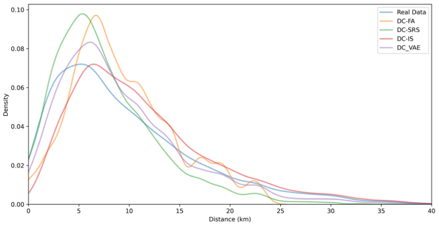
Comparison of trip length distributions.
To ensure a fair and robust comparison, kernel density estimation with a standardized bandwidth was applied to smooth all distributions consistently, and the analysis was restricted to the range of 0–40 km, which covers the most relevant distances in the dataset. The KL divergence results demonstrate that the DC-VAE model achieves the smallest divergence (0.0197), indicating the closest match to the real data. The DC-IS and DC-SRS models follow with divergences of 0.0694 and 0.0891, respectively, showing reasonable alignment but some discrepancies. Conversely, the DC-FA model has the largest divergence (4.8588), highlighting significant deviations from the real data. These findings confirm that the DC-VAE model not only visually aligns better with the real data but also statistically provides the most accurate representation of travel distance distributions.
Further illustration of the comparison of distance distributions between origin and destination across the four models and the real data using box plots (Figure 8) provides additional insights. The real data show a relatively wide spread with a median distance around 10 km and a broad interquartile range (IQR), indicating significant variability in travel distances. Several outliers at longer distances highlight the diversity of observed destination choices.
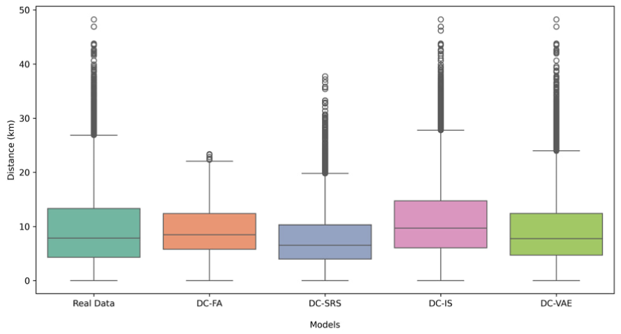
Distance frequency distribution comparison across models and real data.
The DC-FA model underestimates the spread of the real data, with a narrower IQR and a lower median distance. It fails to effectively capture longer-distance choices, as shown by the smaller number of outliers. This misrepresentation may stem from its rigid assumption of equal availability for all alternatives, which disregards key behavioral factors. The DC-SRS model shows a spread closer to the real data than DC-FA but has a slightly lower median. It captures some longer-distance choices but does so less effectively than the real data, as evidenced by a smaller number of outliers and a flatter distribution overall. The DC-IS model demonstrates notable improvements over both DC-FA and DC-SRS. It has a wider IQR and a median that is closer to the real data. Additionally, it captures a reasonable number of outliers, representing longer-distance trips more accurately. However, DC-IS slightly overestimates choices at longer distances, which introduces some deviations from the real data. The DC-VAE model aligns most closely with the real data, effectively capturing the median, IQR, and outliers. It replicates the spread of travel distances observed in the real data and accurately represents longer-distance trips.
Overall, the box plot analysis highlights that DC-VAE is the best-performing method, as it most closely matches the observed variability and central tendency of the real data. DC-IS follows as the second-best method, with noticeable improvements over DC-SRS and DC-FA. This analysis reinforces conclusions from the density plot comparison, further confirming that the VAE-based model offers the most effective approach for capturing realistic destination choice behavior.
Conclusions
This study has explored the potential of using VAEs to enhance choice set generation in destination choice models, focusing on home-based work trips in Montreal, Canada.
The VAE method integrates variational Bayesian techniques with autoencoders to estimate the probability distribution for the underlying choice set generation process, aiming to maximize the likelihood of including the chosen alternatives in the choice set. Initially, the VAE maps alternatives to a lower-dimensional latent space using an encoder model, then generates new alternatives with a decoder model based on these latent representations. The choice set is implicitly created by sampling from this latent space and feeding the samples into the decoder model. Additionally, the VAE model can produce the implicit perception measure when generating new alternatives.
The findings from this study revealed the VAE model’s capability to effectively capture the underlying distribution of chosen alternatives, producing plausible and diverse alternatives. This capability was demonstrated through density plots and CDFs, which exhibited a high degree of similarity between the chosen and generated alternatives. Such visual and quantitative alignment suggests that VAE can mimic the decision-making process of individuals, thereby generating realistic and varied choice sets that enhance the robustness of the destination choice model. This alignment underscores VAE’s potential to address the biases and limitations associated with traditional deterministic and stochastic methods which often fail to capture the full spectrum of potential alternatives.
Moreover, the application of the VAE method to generate choice sets for destination choice models was validated using real-world data and several model structures: DC-FA, DC-SRS, DC-IS, and DC-VAE. The results indicated that models utilizing VAE-generated choice sets (DC-VAE) outperformed those with traditional choice sets with regard to model fit and predictive accuracy. Specifically, the model’s
While this study focused on destination choice modeling for home-based work trips, future research should extend the VAE-based approach to other trip types and different urban areas. This would involve comparing the prediction accuracy of discrete choice models with choice sets generated by VAEs across various contexts and trip purposes. Additionally, using actual job data instead of resident occupation data for census tracts may provide more explanatory power in destination models, making it a valuable direction for future research. Future studies should also examine the performance of destination choice models with various choice set sizes generated by different methods. This would help identify the optimal choice set size and method that balances model complexity with predictive accuracy. Furthermore, integrating VAEs with other DL techniques developed for choice modeling (e.g., Wang et al., Wong and Farooq, and Kamal and Farooq) could enhance model performance and predictive accuracy ( 46 – 48 ).
Investigating whether the training process of the VAE and the ML-based choice modeling can be done simultaneously presents an exciting opportunity. This simultaneous training could streamline the modeling process and potentially lead to even more-accurate and efficient models, as the generative and predictive components would be optimized together. Another future direction could be to adopt other methods for choice set generation in route choice modeling, such as Metropolis-Hastings-based sampling and path size logit-based sampling, for choice set generation in destination choice modeling ( 49 , 50 ). Comparing these methods with the VAE approach would help understand their relative strengths and weaknesses in this new context. It is also important to note that the methods explored in this study rely on sampling mechanisms, meaning their outputs may vary across replications. In this study, because of the computational burden of estimating multiple discrete choice models for each method, we conducted a single full replication per approach. While this setup was sufficient to highlight clear differences in predictive performance and behavioral realism across methods, future work should explore multiple replications to better assess the variability and robustness of results.
Although the VAE-based approach shows promise, it also has potential limitations. The quality of generated choice sets depends heavily on the quality and quantity of the training data. Additionally, while the computational complexity of VAEs can be significant during training, they benefit from modern hardware acceleration (e.g., GPUs) and efficient optimization algorithms, making them scalable for large datasets. Compared with stochastic methods, VAEs offer a unified framework for choice set generation that avoids the need for iterative sampling during inference. Future work should explore techniques for further optimizing VAE training and evaluating the impact of different data preprocessing methods on choice set generation.
Footnotes
Acknowledgements
The authors would like to thank Autorité régionale de transport métropolitain (ARTM) for providing the origin-destination survey data used in this study.
Author Contributions
The authors confirm contribution to the paper as follows: study conception and design: H. Haghi, Z. Patterson, B. Farooq; data collection: xxx; analysis and interpretation of results: H. Haghi, Z. Patterson, B. Farooq; draft manuscript preparation: H. Haghi, Z. Patterson, B. Farooq. All authors reviewed the results and approved the final version of the manuscript.
Declaration of Conflicting Interests
The authors declared no potential conflicts of interest with respect to the research, authorship, and/or publication of this article.
Funding
The authors disclosed receipt of the following financial support for the research, authorship, and/or publication of this article: This research was supported by the Canada First Research Excellence Fund and the Bridging Divides program funded under it.