Sage Journals: Discover world-class research

Abstract

This research is aimed at evaluating the effect of influencing parameters on the dynamic load allowance (DLA) for steel composite bridges subject to autonomous truck platooning (ATP). A comprehensive literature review is presented on platooning configurations and their effect on bridges, the selection of candidate trucks to constitute ATP, and DLA analyses. Next, the modeling of trucks, the road surface roughness generation in MATLAB, and its realization in Abaqus® as 3-D finite element modeling is presented in detail. A parametric study of the DLA is performed for a single span steel girder bridge for a single truck and platoons with two or three trucks, with speed ranging from 60 to 100 km/h, inter-truck spacings between 6 and 10 m, and three road surface roughness profiles (ISO 8608 profile A, ISO 8608 profile B, and ISO 8608 profile C). The results indicate that the resonance of the bridge can be excited by truck platoons for specific speed and inter-truck spacings, which can increase the dynamic load allowance relative to that of a single truck. Combinations of platoon speed and spacing that result in resonance conditions and high DLA vary as a function of surface roughness. When resonance conditions are not encountered, and inter-truck spacings are small, such that all platoon trucks are simultaneously on the span, the DLA is smaller compared with a single truck for smooth surface profiles. Large inter-truck spacings for two-truck and three-truck platoons result in high DLA but lower static loads, which can result in dynamic effects that are not within current Canadian Standards Association (CSA) guidelines, especially for large road surface roughness. ATP on a smooth profile result in only marginal increases of the DLA compared with a single truck and are within current CSA S6 guidelines.

Keywords

autonomous truck platoons dynamic load allowance vehicle–bridge interaction pavement surface roughness CSA S6

Cooperative adaptive cruise control is a promising technology that allows trucks to form platoons with short inter-truck distances using wireless inter-truck communication ( 1 ). Truck platooning is largely accepted by relevant parties because of its potential to reduce greenhouse gas emissions and save fuel. Computational fluid dynamic studies show that driving at closer inter-truck spacing decreases drag forces on the trucks behind the leading truck considerably ( 2 ) and reduces fuel consumption for the leading and trailing trucks ( 3 ). Depending on the platoon parameters, the fuel consumption economy can vary between 7% and 28% for a two-truck platoon (3, 4). The trucking industry accounted for 71.5% of freight transportation in the United States in 2017 (and 72.7% in 2024 according to the American Trucking Association) which implies that significant economic and environmental benefits could be harnessed by the introduction of platooning ( 5 ). Furthermore, given the close spacing between the trucks, platooning reduces the frequency of traffic congestion ( 6 ) and increases traffic throughput ( 7 ). However, concerns about platooning have been raised because of negative impacts on traffic safety resulting from visual obstructions to signage ( 8 ), impacts on lateral traffic safety ( 9 ), and increased pavement distress ( 10 ). To fully realize benefits from autonomous truck platooning (ATP), sophisticated fleet planning and platoon operations would have to be formulated and implemented by the trucking industry ( 1 ). Besides operational issues, the adequacy of the existing infrastructure, in particular bridges, to accommodate the loads from ATP requires investigation to propose fully informed guidelines with regard to the deployment of platooning technology in the transportation system. It is reported that introducing truck platooning at closer spacing could pose a potential risk of structural inadequacy for bridges with lower rating factors ( 11 ).

Sajid et al. investigated the influence of live loads from ATP on the reliability of bridges designed according to existing bridge design guidelines such as the American Association of State Highway and Transportation Officials Load Factor Design (AASHTO LFD) and the AASHTO Load and Resistance Factor Design (AASHTO LRFD) ( 12 ). The study showed that the dynamic amplification factor (or dynamic load allowance) currently given by the AASHTO LRFD ( 13 ) may be conservative for ATPs. This research has a similar objective specific to the Canadian context and the potential impact on the relevant CSA S6, Canadian Highway Bridge Design Code (CHBDC) provisions. The current consensus is that the DLA is expected to be lower with an increase in the number of closely spaced trucks because of the increased static load (14 –16) but needs to be substantiated for the ATPs. This study is aimed at performing an in-depth review of the relevant literature and investigating the causative relationships of different parameters such as coefficient of surface roughness, number of trucks, and inter-truck spacing with the dynamic load allowance using parametric studies and 3-D finite element modeling. A schematic of the extent of the study is shown in Figure 1.

Figure 1.

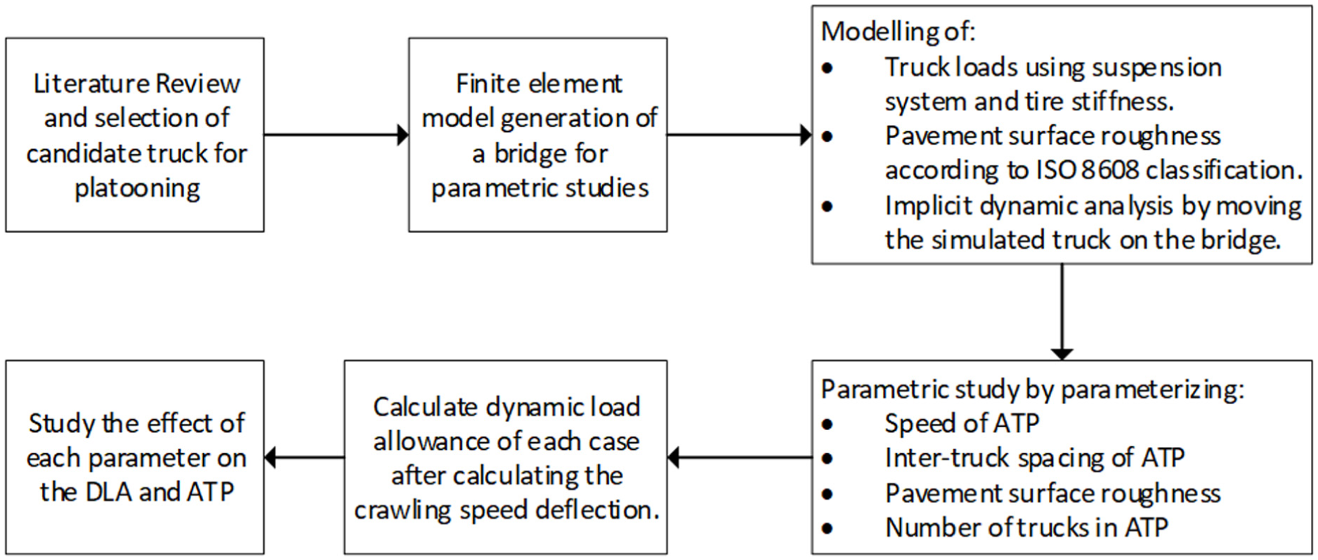
Flow chart of the sequence of research.

Review of Literature on Autonomous Truck Platooning

Autonomous truck platooning has been the focus of significant research interest in the transportation industry over the past decade. In particular, frameworks and models have been proposed to quantify the influence of truck platoons on existing bridges ( 17 ). Most of these are parametric studies on the effect of platoons on the safety of bridges designed according to the existing standards ( 18 – 21 ). Yarnold and Weidner (01) performed a parametric study on the distribution of the shear force and bending moment from truck platoons formed with C5 standard trucks of the Florida Department of Transportation (DOT). A line girder analysis for simply supported and continuous beam systems was performed and bending moments and shear forces were obtained as a function of span length and headway distance between trucks in the platoon; these were then compared with AASHTO LRFD live loads. Concerns were raised for loads on long-span bridges with closely spaced truck platoons. These findings are consistent with those reported by Sajid et al. ( 12 ) and Ling et al. ( 22 ). Tohme and Yarnold ( 19 ) performed analytical and parametric load rating studies for steel bridges subjected to truck platoons. They used a benchmark bridge from the Manual of Bridge Evaluation (MBE) ( 23 ) and performed parametric studies to evaluate the ratio of load ratings from platoons to design load ratings and legal load ratings. The authors reported that allowable stress ratings (ASRs) may be reduced in the positive bending moment region for all the combinations of platoon headways (6 to 12 m) and span lengths (32 to 68 m) considered in the study. Likewise, the ratings may be reduced in the negative moment regions for most span lengths ( 19 ). Similarly, the load factor ratings (LFRs) were adequate for truck platoons in the positive moment region and less so in the negative moment regions for all span lengths. Elshazli et al. have reported results from around 29,000 computer simulations by parameterizing different characteristics of platoons ( 24 ). They have identified the number of trucks in the platoon and the headway spacing as the main critical parameters influencing the bridge rating ( 25 ). Braguim et al. studied the possibility of reducing fatigue damage in steel girder bridges by allowing truck platooning ( 21 ). They performed line girder analyses for sets of truck platoons on simple and continuous span bridges. The stress range and number of cycles were recorded using rainflow counting, and Miner’s rule was used to quantify the fatigue damage. The fatigue damage for different platoon configurations was normalized relative to the AASHTO LRFD fatigue loads for comparison. Although load effects were increased by platooning, the number of stress cycles was reduced because of the synchronized movement of trucks, which in some cases contributed to decreased fatigue damage. Thulaseedharan and Yarnold performed a study for the prioritization of prestressed concrete bridges in Texas for the deployment of platooning ( 26 ). Truck platoon load ratings were used as well as National Bridge Inventory (NBI) structural evaluation condition ratings to prioritize each bridge for detailed evaluations before authorizations for truck platoons.

Wassef ( 27 ) reported on the potential candidate trucks for platooning in a comprehensive study, which includes most of the trucks used by Yang et al. ( 28 ) in their study. However, the Florida DOT C5 trucks were not included by Wassef ( 27 ) as a potential candidate truck, which was reported in earlier studies on platooning ( 19 , 20 ). Yang et al. ( 28 ) performed a parametric study on the influence of variability (CoV) of platoon loads, the headway spacing, span length, and live load factor on the safety of selected bridges (simple and two-span continuous each with six different span lengths ranging from 9.14 to 61 m) designed using the AASHTO LRFD specifications ( 28 ). The effect of bias factors is studied in an aggregate sense in their research; however, the dynamic amplification factor was not parameterized to evaluate its effect on bridge safety. Furthermore, the bridges studied were limited to those designed using the AASHTO LRFD provisions.

In a sensitivity study for the reliability analysis of a steel composite bridge, Sajid et al. determined the safe deployment of ATPs relative to both AASHTO LRFD and LFD bridge design guidelines on current bridges ( 12 ). They calculated reliability indices for steel composite bridges that followed both AASHTO guidelines for diverse settings of ATP live loads by parameterizing the variability, bias, and dynamic amplification ( 12 ). It should be noted that the statistical parameters were also taken into account in an aggregate sense by using load factors by Steelman et al. ( 29 ) for both AASHTO LRFD and AASHTO LFD bridges. Sajid et al. ( 12 ) used the bias factor and coefficient of variation (CoV) in isolation to evaluate their separate effects. It was reported by Sajid et al. ( 12 ) that the reliability could be significantly influenced by the DLA factor currently stipulated in the AASHTO LRFD Bridge Design Specifications ( 13 ). Braley studied bridge deflection under platooning trucks as a function of the number of trucks for two different truck spacings ( 30 ). It was reported in their study that increasing the number of trucks in the platoon would reduce the bridge deflection as is reported in other studies, for instance ( 14 ). Nevertheless, the effect of resonance on the platooning trucks was not specifically studied since only one surface roughness profile was investigated in their study ( 30 ).

In general, the current literature indicates that an increase in the number of trucks on a bridge decreases the DLA because of the increase in the total static load. The CSA S6 provisions describe the DLA in an equivalent static load that is a fraction of the CL-W Load (an idealized five-axle truck used for the purpose of design by CHBDC). It also suggests that increasing the number of trucks will reduce the DLA on the bridge ( 31 ). However, Ling et al. reported that the platooning trucks can excite resonant frequencies on some bridges, which results in an increase in DLA above the levels specified in the Chinese, Euro, and AASHTO LRFD codes ( 32 ). In a later study, Ling et al. propose an increase in DLA factors for small- and medium-span concrete bridges in the Chinese code based on the results obtained for four truck platoons ( 33 ).

Dynamic Load Allowance Provisions by Current Design Guidelines

Different bridge design guidelines provide dynamic amplification factors either as a constant value, as a bridge span length, as a function of span length and bridge deck thickness, or as a function of fundamental frequency. In the CHBDC guidelines, the dynamic amplification depends on the fundamental frequency as shown in Figure 2. The DLA is also dependent on the number of axles, and is applied to the CL-W truck. It suggests the use of component level DLA factors as provided in Table 1. In the CSA S6 commentary, the dynamic amplification is partially dependent on the fundamental frequency, as shown in Figure 2. The corresponding fundamental frequency ( $f_{0}$ ) can be calculated for a given span length ( $L$ ) of a bridge using Equation 1 given by ( 34 ) and ( 35 ).

f_{0} = 82 L_{\max}^{- 0.9}

(1)

Figure 2.

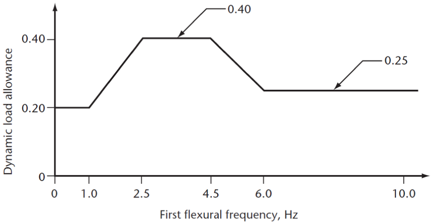
Dynamic load allowance as a function of frequency ( 31 ).

Table 1.

Dynamic Load Allowance for Components other than Buried Structure ( 31 )

S. No.	Component	Dynamic load allowance
1	Deck Joints	0.5
2	Spans where only one axle of the CL-W Truck is used (except for deck joints)	0.4
3	Spans where any two axles of the CL-W Truck, or axles nos. 1 to 3, are used	0.3
4	Spans where three axles of the CL-W Truck, except for axles nos. 1 to 3, or more than three axles, are used	0.25

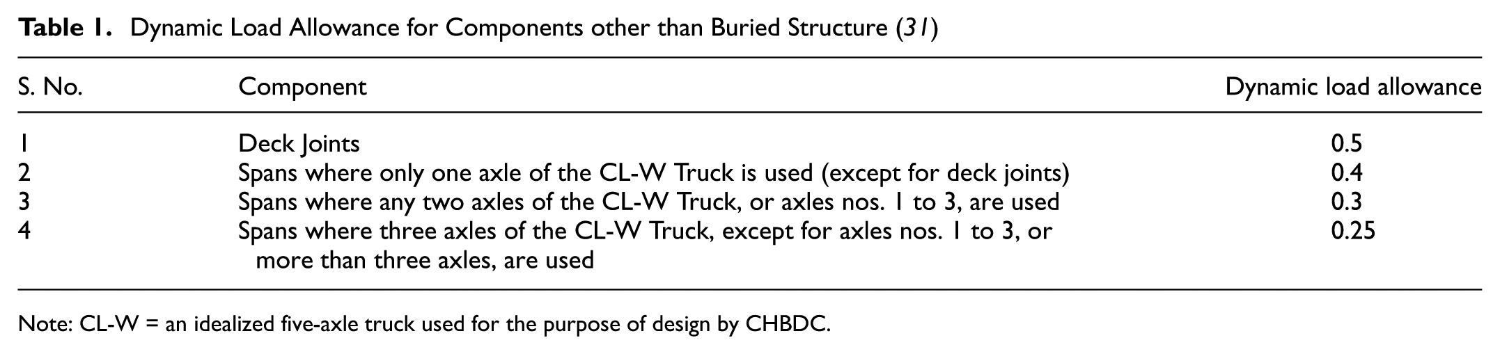
Note: CL-W = an idealized five-axle truck used for the purpose of design by CHBDC.

The AASHTO Standard Specifications for Highway Bridges (2002) provides the following equation to calculate the dynamic amplification factor (also known as impact factor [I]) in which L is the span length (in feet) ( 36 ).

I = \frac{50}{L + 125} \leq 0.3

(2)

According to the AASHTO LRFD (2017) specifications, the DLA at desk joints for all limit states is 75% and 15% for all other components for fracture and fatigue limit states. For all other limit states, it is taken as 33% ( 13 ). The British Standards also use a constant DLA (known as impact factor) of 25% ( 37 ).

The Eurocode on the other hand uses the dynamic amplification factor (DAF) based on either shear force or bending moment. The factor, which is a function of span length and number of lanes, is included in the load values specified in SS-EN 1991-2 Part 2: Traffic loads on bridges. For single lane bridges, the DAFs are given by Equations 3 and 4 and for a two-lane bridge for both moment and shear, the DAF is given by Equation 5. For a four-lane bridge, the DAF of 1.1 is recommended.

DA F_{bending moment} = {\begin{matrix} 1.7 L \leq 5 m \\ 1.85 - 0.03 L 5 m < L < 15 m \\ 1.4 L \geq 15 m \end{matrix}

(3)

DA F_{shear force} = {\begin{matrix} 1.4 L \leq 5 m \\ 1.45 - 0.01 L 5 m < L < 25 m \\ 1.2 L \geq 25 m \end{matrix}

(4)

DAF = {\begin{matrix} 1.3 - \frac{0.4}{100} L L \leq 50 m \\ 1.1 L > 50 m \end{matrix}

(5)

Currently, the British Standard and CHBDC S6 uses a DLA of 1.25, while the AASHTO LRFD uses 1.33. A more detailed review of the national code provisions for the DLA of different jurisdictions is provided in ( 38 ). However, the review does not address platooning trucks moving synchronously on a bridge.

Finite Element Modeling

The finite element method (FEM) code, Abaqus® is used in this paper to model a steel girder bridge similar to the one analyzed in ( 15 ). The general-purpose linear brick element C3D8R was selected. The mesh size for bridge deck and girders was respectively used as 200 and 250 mm after convergence analysis. The steel girders are connected to the concrete slabs using tie constraints. The bridge has five 36.6-m long W40 x 264 girders spaced at 1.625 m (on center) that are simply supported on both ends, with diaphragms every 9.144 m. The girders are supporting a 177.8-mm (thickness) by 8.128-m (wide) bridge slab. The girders are modeled using 413-MPa steel and 55.16-MPa concrete for the slab. The eigen value analysis of the modeled bridge gives resonant frequencies of 1.90 Hz, 2.90 Hz, and 8.20 Hz respectively for the first bending mode, first torsional mode, and second torsional mode. It is worth noting that this model is generated for computational purposes in the parametric study as has been used in other similar studies, such as ( 15 , 32 , 39 ), without field validation. Further, this bridge in the model is for demonstration purposes and changing the geometrical or mechanical parameters will provide different results. The dynamic analysis of the bridge is performed by considering the vehicle–bridge interactions and road surface roughness. The methodologies adopted for modeling both are explained below.

Truck Load Modeling

Selection of Candidate Truck

The selection of a candidate for constituting the platooning is performed in light of the review of candidate trucks. The predominantly used truck in the studies cited above is FHWA Class 9 truck. Wassef ( 27 ) analyzed the weigh-in-motion data sets for different trucks in various states of the United States. The results in Figure 3 show that the predominant truck is FHWA Class 9, which is a five-axle truck. The evidence given in Figure 3 is also reported in previous studies found in the literature ( 40 ). Other researchers have used different trucks in their studies related to platooning. Some of these studies along with the types of trucks they used are shown in Table 2. In all these cases, FHWA Class 9 is shown as a suitable option to act as a candidate truck in homogenous ATPs in future and therefore it is selected as a model for further studies in the literature.

Figure 3.

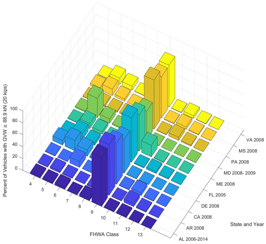
Percent of vehicles for different FHWA classes having gross vehicle weights greater than 88.9 kN for different states in the United States in a particular year. The figure is created using the data set provided in ( 27 ).

Table 2.

Trucks Used to Constitute Platoons in Various Published Studies

Authors	Main premise of research	Truck(s)	Reference
Sajid et al.	Reliability analysis of steel composite bridges subject to ATP	FHWA Class 9 Florida DOT C5 NJTA Type 3S2	( 12 )
Yang et al.	Effects of platooning on girder bridges	FHWA Class 9 Type 3-3 NJTA Type 3S2 Notional rating load	( 28 , 29 )
Yarnold and Weidner	Static load effects of truck platooning on steel girder bridges	Florida DOT C5	( 20 )
Tohme and Yarnold	Load rating of steel girder bridges owing ATP	Florida DOT C5	( 19 )
Ling et al.	Dynamic impact of platooning loads on brides subjected to Platoons	Florida DOT C5 Chinese five-axle Truck European five-axle Truck	( 32 )

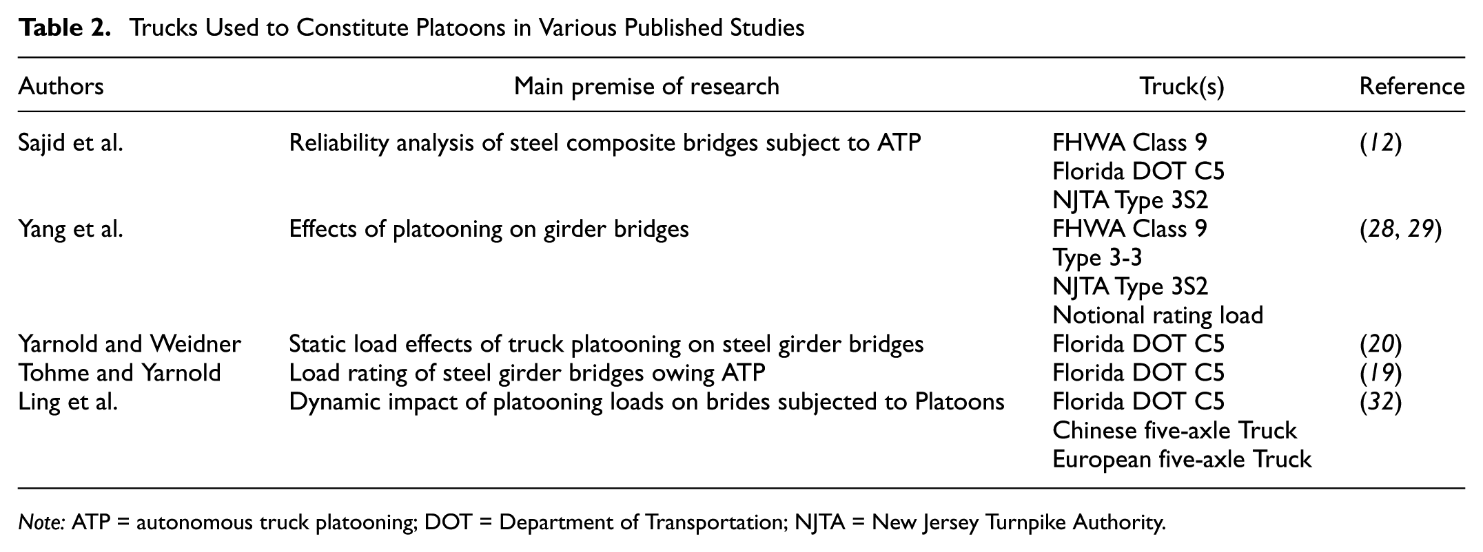
Note: ATP = autonomous truck platooning; DOT = Department of Transportation; NJTA = New Jersey Turnpike Authority.

Modeling of Truck Loads

The truck loads can be modeled as simple point masses to full 3-D finite element models of trucks. The full 3-D models of trucks are generally used to analyze loads in impact (crash) studies. Published studies suggest the use of several techniques to model truck loads. The point mass approach is used in ( 15 ) to model vehicle–bridge interaction for calculating the dynamic amplification factor of long-span bridges. In the point mass approach, the axle weights are modeled on the bridge deck and then moved across to simulate the rolling wheels of a truck. A detailed wheel point mass model has six degrees of freedom: vertical displacement, horizontal displacement, lateral displacement, roll, pitch, and yaw. For the DLA studies, only the vertical degree of freedom is considered in the point mass approach since this is the most important parameter for the current problem ( 15 , 32 ). The point mass approach includes a sprung-mass model to represent the stiffness of the truck suspension ( 41 ). Chang et al. proposed a rigid-disc model imitating a wheel, neglecting the tire deformations, connected to the springs on the top ( 42 ). The disc model is proposed given the shortcomings of the point model moving on a rough surface. The rough surface of the pavement is a track of a series of hills and valleys and the point mass may not touch the valley points. The study reported that for the displacement time history, the use of point model to model the wheel and the disc do not result in a significant difference. However, if the velocity or acceleration responses are required, then a disc model should be used as it results in lesser amplitudes ( 42 ). Afia et al. ( 43 ) used dual spring systems to model both the suspension systems and the tire stiffness. This approach takes into account both the stiffnesses of the truck suspension system and the tires. Ling et al. ( 32 ) used a more detailed approach in modeling the truck loads. They incorporated the rolling and pitching moments as well as the truck suspension system and the tire damping stiffness parameters. Furthermore, instead of using a point to apply wheel loads, the points are applied on a patch equal to the width of the tire. However, while this is a potentially more realistic approach, the quantification of the parameters for each of these unknowns can be subjective which may lead to unrealistic responses.

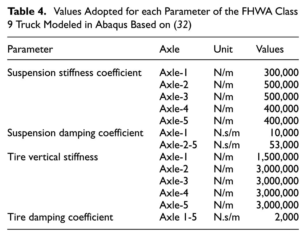
Based on the above reasoning, this paper used a dual system specifying both tire stiffness and damping and the truck suspension system as shown in Figure 4a. More details can be found in ( 44 ). This model closely imitates the quarter car model which is reported in the literature for similar problems ( 43 , 45 ). The axles and their associated loading complying with FHWA Class 9 truck are given in Figure 4b and Table 3 respectively, consistent with the literature. Similarly, the parameters and the parameters adopted to characterize the tires and the suspension system are given in Table 4 in light of Ling et al. ( 33 ). It is worth mentioning that these parameters are not invariantly available in the literature and therefore a more rational approach for normalization or referencing of the final results should be used in order to minimize the uncertainty associated with these values.

Figure 4.

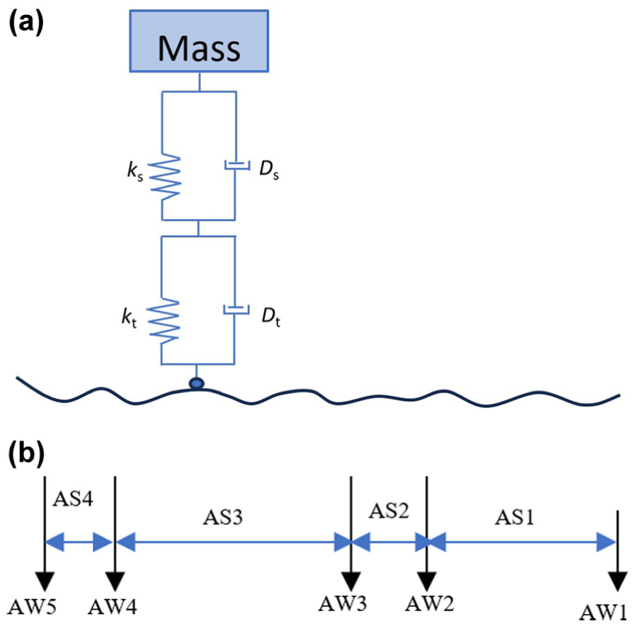
(a) Realization of truck loads from each wheel in the 3-D finite element (FE) model, in which ks, kt, Ds, and Dt are respectively the suspension stiffness, tire stiffness, suspension damping coefficient, and tire damping coefficient; and (b) axle topology of FHWA Class 9 truck ( 12 ).

Table 3.

Axle Spacing and Axle Loads of FHWA Class 9 Truck Corresponding to Figure 5

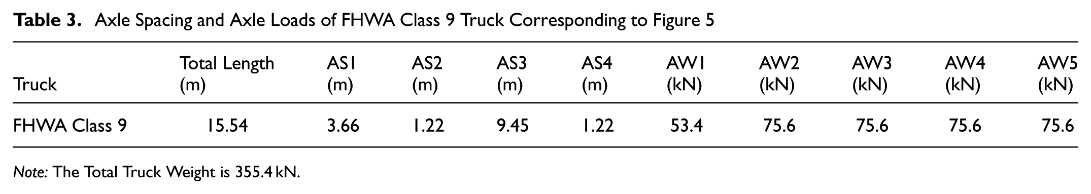
Truck	Total Length (m)	AS1 (m)	AS2 (m)	AS3 (m)	AS4 (m)	AW1 (kN)	AW2 (kN)	AW3 (kN)	AW4 (kN)	AW5 (kN)
FHWA Class 9	15.54	3.66	1.22	9.45	1.22	53.4	75.6	75.6	75.6	75.6

Note: The Total Truck Weight is 355.4 kN.

Table 4.

Values Adopted for each Parameter of the FHWA Class 9 Truck Modeled in Abaqus Based on ( 32 )

Parameter	Axle	Unit	Values
Suspension stiffness coefficient	Axle-1	N/m	300,000
	Axle-2	N/m	500,000
	Axle-3	N/m	500,000
	Axle-4	N/m	400,000
	Axle-5	N/m	400,000
Suspension damping coefficient	Axle-1	N.s/m	10,000
Suspension damping coefficient	Axle-2-5	N.s/m	53,000
Tire vertical stiffness	Axle-1	N/m	1,500,000
	Axle-2	N/m	3,000,000
	Axle-3	N/m	3,000,000
	Axle-4	N/m	3,000,000
	Axle-5	N/m	3,000,000
Tire damping coefficient	Axle 1-5	N.s/m	2,000

Road Surface Roughness Modeling

Generating Road Surface Roughness Profile

The dynamic analysis of the bridge is performed by considering the vehicle–bridge interactions and road surface roughness. Several approaches can be used for the simulation of road surface roughness. The most common are based on either a shaping filter or a sinusoidal approximation (46, 47). The shaping filter approach applies a filter to a white noise signal to reproduce specified statistical properties of the road surface. For the sinusoidal approach, a power spectral density (PSD) function ( 48 ) is used to generate random pavement surface profiles in agreement with the ISO 8608 classification ( 49 ).

The road surface roughness follows a standardized classification system as described in ISO 8608, Mechanical vibration—Road surface profiles—Reporting of measured data. This classification ranges from A to H, where A refers to a smooth road surface, while H refers to a road surface that can only allow crawling speeds ( 50 ). These roughness profiles are a function of the lower and upper limit of power spectral density (PSD) of vertical displacement and PSD of acceleration. Fundamental concepts in ISO 8608 are spatial frequency, road profile, and PSD. Spatial frequency is defined as (cycles/m), contrary to the ordinary unit Hertz (cycles/s). Road profile is the variations in height of the road surface measured along one track on, and parallel with, the road. The roughness coefficient ( $G_{d} (n_{0})$ ) for each class of profile is provided in Table 5 ( 49 ).

Table 5.

ISO 8608 Classification Relative to Roughness Coefficient Values

Road class	$G_{d} (n_{0}) (10^{- 6} m^{3})$
Road class	Lower limit	Upper limit
A	—	32
B	32	128
C	128	512
D	512	2048
E	2048	8,192
F	8,192	32,768
G	32,768	131,072
H	131,072	—

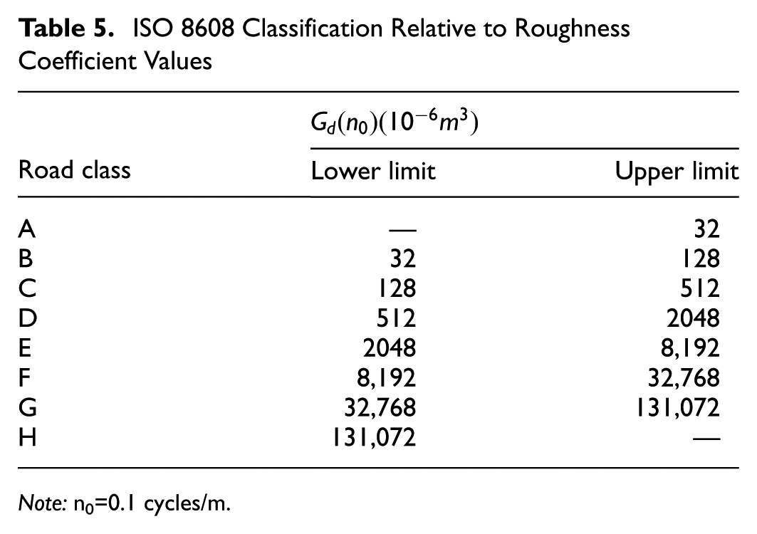
Note: n₀=0.1 cycles/m.

A comparison of different profiles for various classes is provided in Figure 5. It should be noted that the profile generated a random phase angle and a distribution of heights along the longitudinal axis of the bridge. The effect of random phase angle is shown for a single class of surface roughness in Figure 6 for a given profile A-B. It is noted that the random phase angle results in random locations for the “hills” and “valleys” in the profile. The pavement surface roughness profiles are generated using a MATLAB code in light of ( 49 ).

Figure 5.

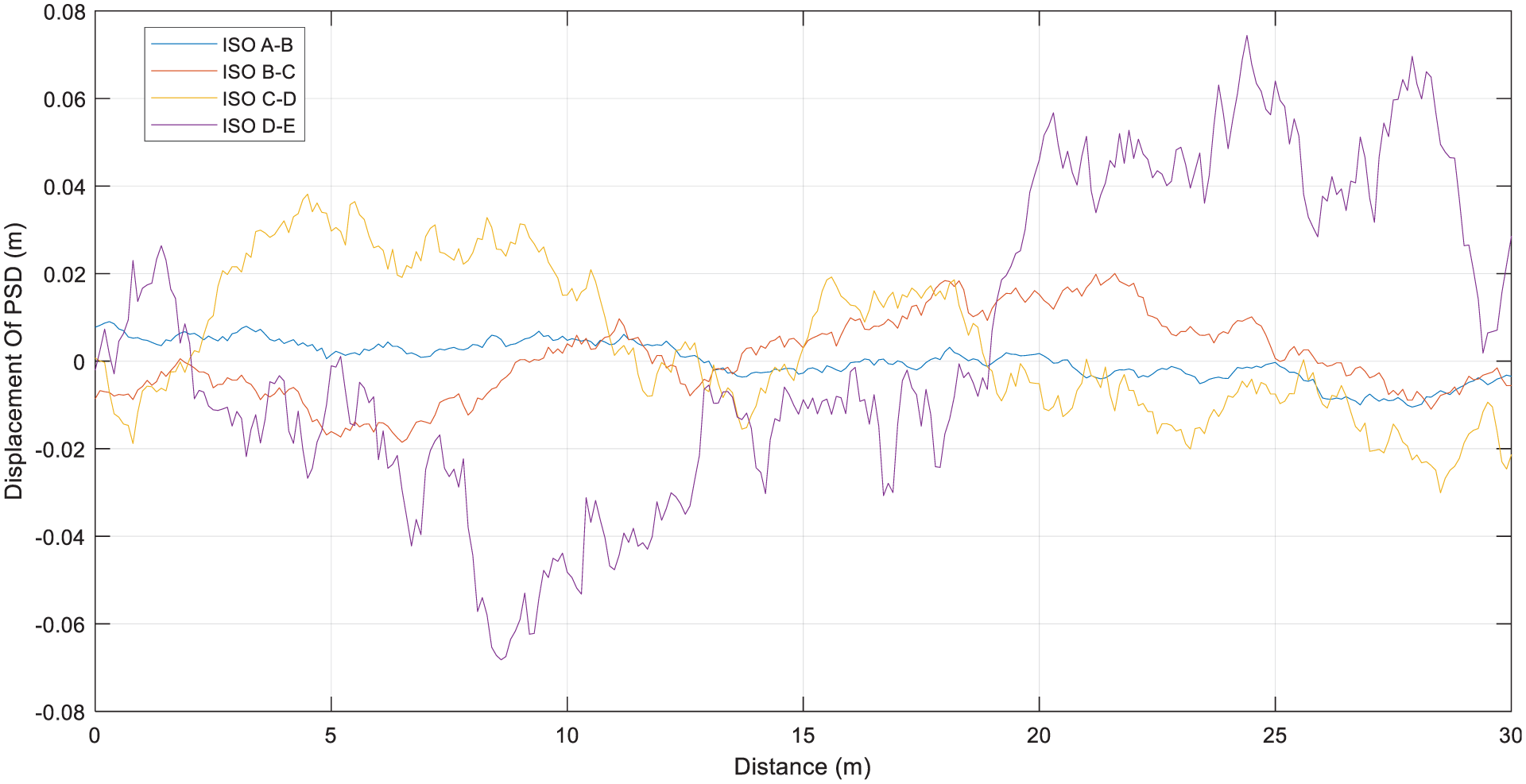
Pavement surface roughness profiles for various roughness classes.

Figure 6.

Effect of random phase angle on the pavement surface roughness profile.

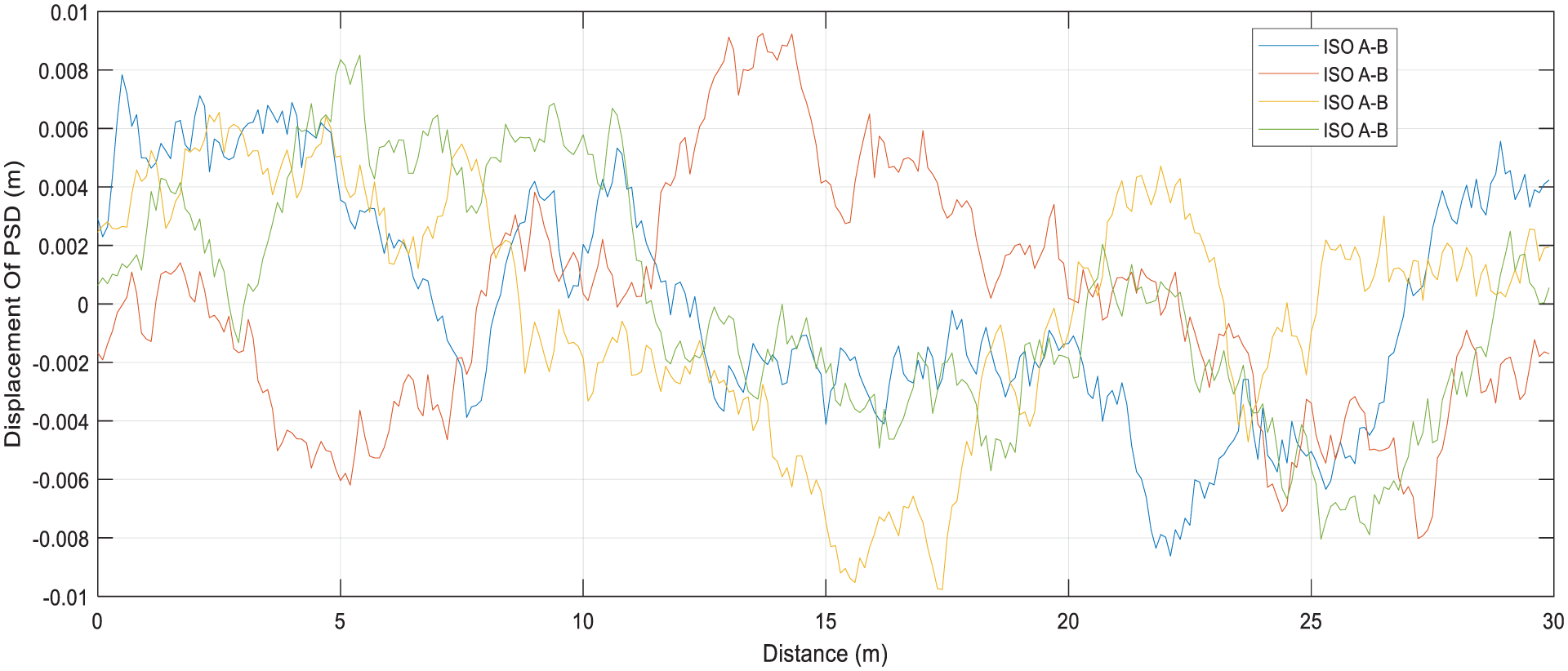
The actual profiles of road surface roughness are classified according to the International Roughness Index ( 51 ) classification system by the World Bank and used in code calibration efforts, such as in NCHRP 368 ( 14 ). The artificial profiles generated according to the classification of ISO 8608 are compared with the actual profiles observed in the field following the IRI classification system by ( 52 ). The sensitivity analysis performed in their study for different parameters of the artificial profiles shows that care should be taken when selecting the inputs to these parameters. In the current paper, the effect of the sampling interval is studied and it is concluded that using a very small sampling interval (of the order 0.01 m) to create the surface roughness profile may not be practical. After some sensitivity analysis, a sampling interval of 100 mm is selected which is consistent with similar studies ( 53 ). The approach for artificial road surface roughness profile generation is consistent with various published studies ( 32 , 33 , 43 , 49 ). For the purposes of this research, three road surface roughness profiles are generated using MATLAB for profile A, B, and C using lower limits of roughness coefficient values for the respective profiles given in Table 5 as shown in Figure 7.

Figure 7.

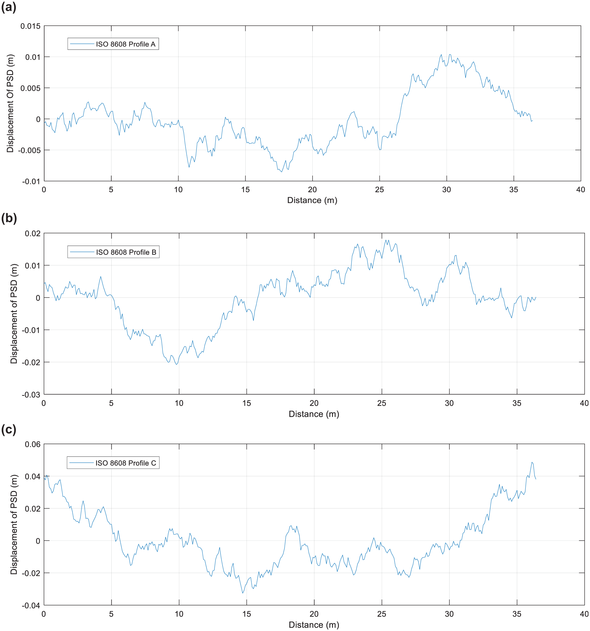
Road surface roughness profiles: (a) ISO 8608 Class A; (b) ISO 8608 Profile B; and (c) ISO 8608 Profile C.

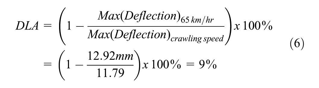
The literature also presents other simplified approaches for the realization of road surface roughness in the finite element code. An example is modeling the surface roughness as total interacting force on the bridge as the sum of weight of the truck and the variation in the vertical interacting force as a result of road surface roughness, the wheel hop, and the associated body bounce vibrations ( 15 ). The wheel hop is a result of the bump at the bridge entrance, which produces an impact that results in vibrations in the range of 16 Hz from the wheels independently from the truck body ( 54 ). This vertical interacting force is taken as 10% of the weight of an HS-20 truck and the resulting vertical interacting force is generated using a sinusoidal function for a rear axle weight of 8 tons (16 kips) and 10% variation. This example is implemented in Abaqus® for the composite bridge modeled above, which results in the maximum deflection of 12.92 mm under truck load at 65 km/h compared with 11.79 mm under crawling speed. The DLA obtained was 9% as shown in Equation 6.

\begin{matrix} DLA = (1 - \frac{Max {(Deflection)}_{65 km / hr}}{Max {(Deflection)}_{crawling speed}}) x 100 % \\ = (1 - \frac{12.92 mm}{11.79}) x 100 % = 9 % \end{matrix}

(6)

The issue in this approach, however, is the lack of relationship between the variation of the vertical interacting forces and the ISO 8608 categorization of roughness profiles. Another example is modeling the surface roughness by generating roughness profiles using a PSD approach for a particular ISO 8608 surface roughness category and then calculating the vertical force as a PSD profile value at that instant, and the stiffness of the suspension system of the passing truck, and subsequently model its vertical forces at each instant of time ( 43 ). For multiple trucks, however, this approach can be inefficient.

Implementation of Road Surface Roughness Profile in Finite Element Tool

The roughness profiles generated using MATLAB are implemented in Abaqus® on the bridge deck for the parametric studies which are explained in the following section. First, the generated road surface roughness profile heights for each interval of longitudinal length of bridge deck are used to generate a 3-D matrix. The heights only change in the longitudinal direction of the bridge deck and they are constant in the lateral direction (which is the transverse of the bridge deck). This modeling strategy is consistent with a similar published study ( 55 ). Following this, a recent tool—RufGen ( 56 ) in Abaqus®—is used to import the generated 3-D profile for each case. An alternative procedure for rough surface generation is writing a user-defined subroutine in Abaqus®, which can be a daunting task. The RufGen plug-in is used to import the surface roughness as an orphan mesh from which a part is created using Create Geometry from Mesh plug-in in Abaqus®. Subsequently, the interactions are defined to assign this part to the bridge deck to characterize the surface roughness. A typical surface roughness defined on bridge deck is shown in Figure 8. This is generated using ISO 8608 Class C profile.

Figure 8.

Close up of the side of the exterior girder and bridge deck to show the roughness variation in the transverse and longitudinal direction of bridge deck.

Following the road surface roughness definition in Abaqus®, the truck wheels are simulated at a given speed on the exterior lane of the bridge deck and implicit dynamic analysis is performed to obtain the deflection time history at the mid-point of the exterior girder. The exterior lane and exterior girders are selected as they undergo the highest deflection under truck loads ( 55 ).

Numerical Simulations

The methodology adopted for this work is outlined in Figure 9. The process starts by developing a numerical model of a steel composite bridge in Abaqus® from the published literature ( 15 ). The bridge is confirmed for its accuracy using frequency analysis in Abaqus®. Subsequently, FHWA Class 9 truck is selected to constitute different truck platoon arrangements with different inter-truck spacings and number of trucks. The inter-truck spacing is defined as the distance between the rear axle of the front truck and the front axle of the rear truck. The lower inter-truck spacing of 6 m selected here, consistent with similar studies such as ( 12 ), creates the worst-case scenario of loading on the bridge but such configuration may create heating problems for engines in rear trucks caused by reduced air-flow and its practical implementation should take that into account. Next, platoons are generated and driven across the bridge on exterior lanes. Each of these generated platoons are then driven across the selected bridge with simulated profiles A, B, and C respectively (using the ISO 8606 classification) at five different speeds in the range of 60 to 100 km/h. In addition, the platoons are moved at crawling speeds to calculate the DLA for each case. Given the crawling speeds of platoons also exhibit vibration of the bridge deck, which is expected, a moving average filter must be used to dampen the deflection time history. However, this approach is computationally more expensive. Alternatively, the centroid of the axle loads is obtained and the platoons are placed on that bridge according to that location and static analysis is performed to obtain maximum deflection at mid-span on the exterior girder. The comparison found the latter approach to be more computationally efficient and to involve less subjectivity since the former would require the selection of order of the filter to completely damp out the fluctuations in the deflection time history and therefore the latter was selected. The set of simulations forms the data set for the analysis of the DLA as a function of speed, inter-truck-spacing, roughness of profiles and number of trucks in a platoon.

Figure 9.

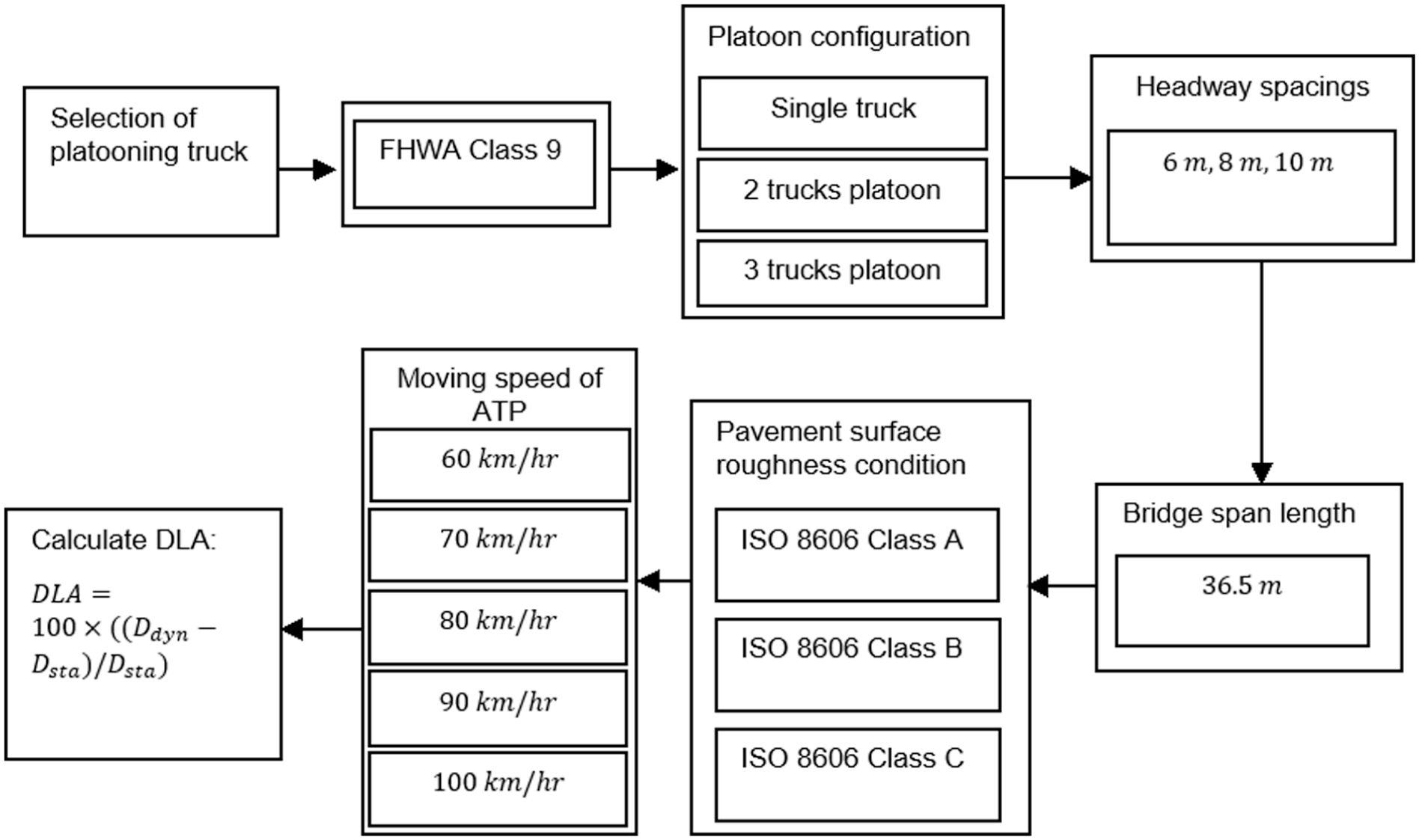
Flow chart of the parametric study and overall methodology for data generation.

The deflection time histories are generated following numerical simulations for each case outlined in Figure 9. Some selected deflection time histories with different characteristic parameters are shown in Figure 10.

Figure 10.

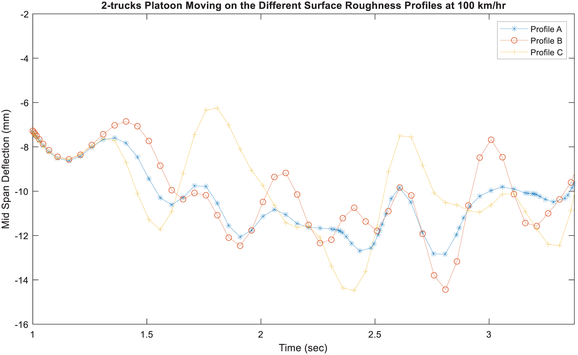
Deflection time histories from selected simulations comparing the effect of road surface roughness intensities characterized by various ISO 8608 profiles. The two-truck platoons have consistent inter-truck spacing of 8 m for all three cases.

Results and Discussion

The parametric analyses are performed to generate data according to the flow chart given in Figure 9. The DLA of 0.25 corresponds to the value recommended in the commentary of the Canadian Highway Bridge Design Code CSA S6.1-19, C3.8.4.5) and is provided as a reference for comparison purposes. First, the DLAs of single trucks on different surface roughness profiles are obtained and compared with the DLA proposed by CHBDC S6 guidelines for various speeds (Figure 11). It can be noted that in all cases, the calculated values are within the limits stipulated by the CSA S6 ( 31 ) provisions except for profile C. As expected, the surface roughness directly influences the DLA values. However, this relationship is not linear as can be noted from Figures 12 –14. For instance, if profile A is considered, the speed values directly influence the DLA from 60 to 80 km/h, but this trend reverses above 80 km/h. Ling et al. ( 32 ) reported resonance for this span length at 80 km/h which is the reason for this trend for the single truck moving on the bridge.

Figure 11.

Dynamic load allowance (DLA) of single trucks modeled on different surface roughness profiles in comparison with CSA S6 provisions.

Figure 12.

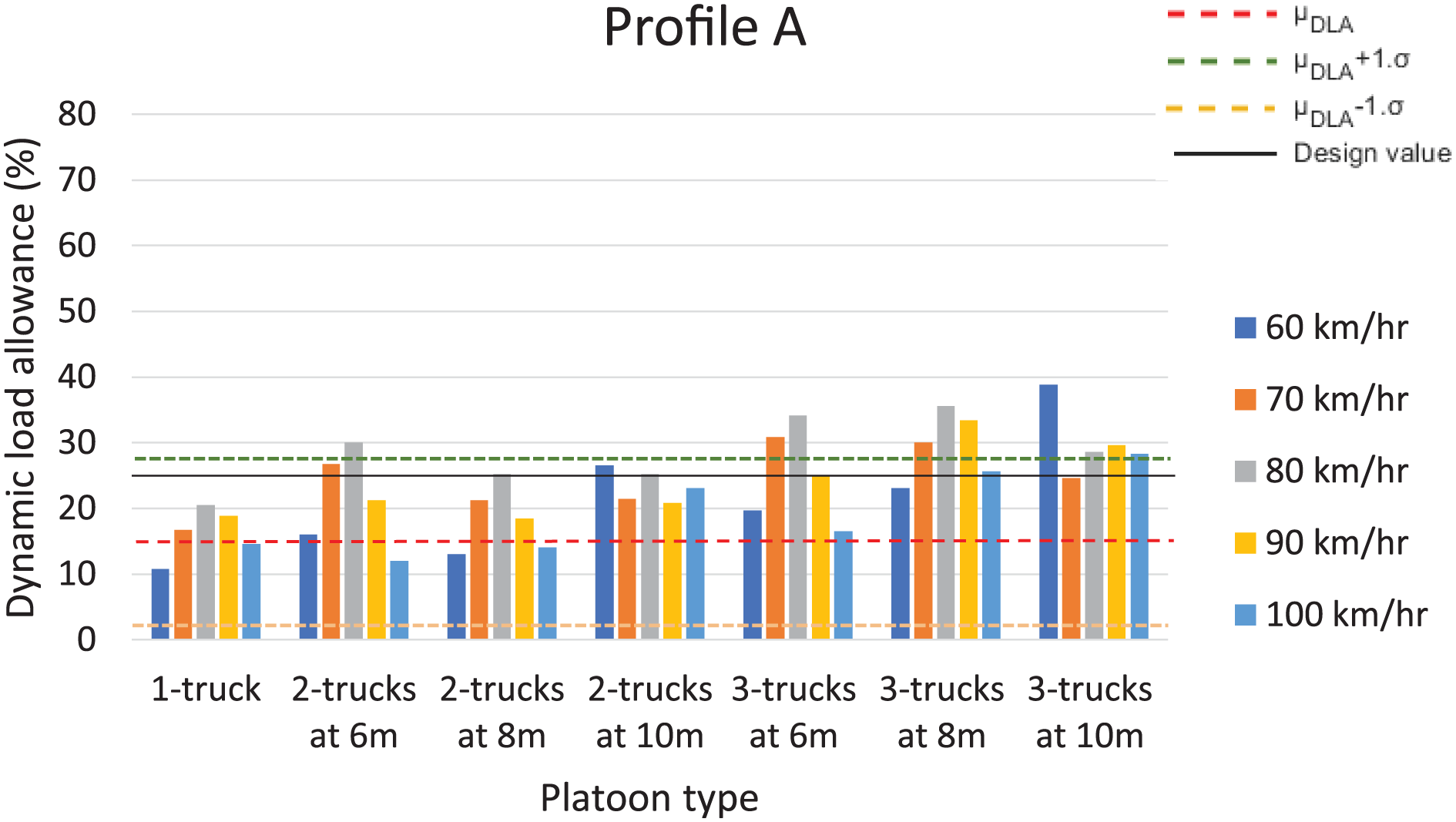
Dynamic load allowance (DLA) of different platoon trucks configurations on surface roughness profile A.

Figure 13.

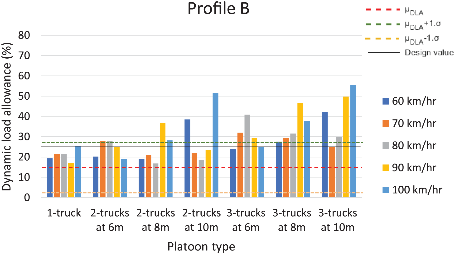
Dynamic load allowance (DLA) of different platoon trucks configurations on surface roughness profile B.

Figure 14.

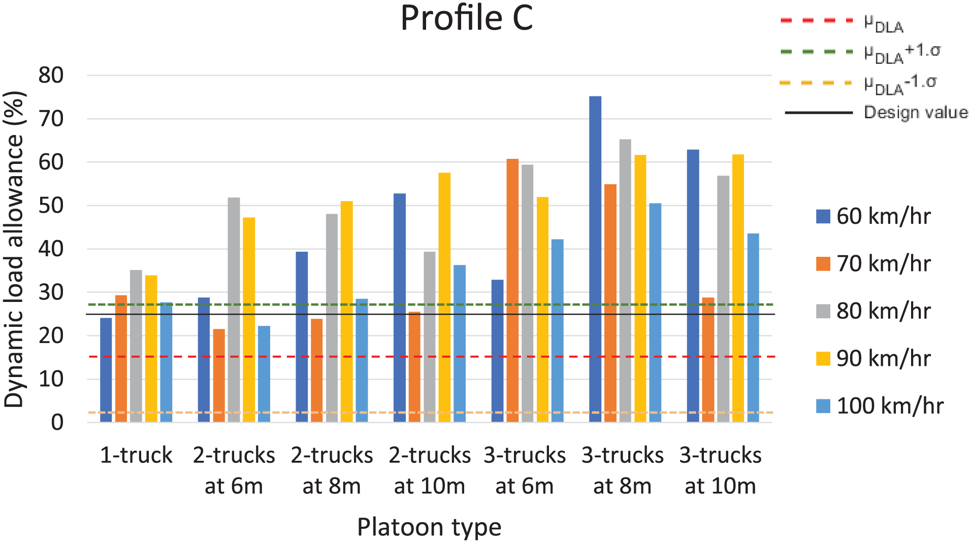
Dynamic load allowance (DLA) of different platoon trucks configurations on surface roughness profile C.

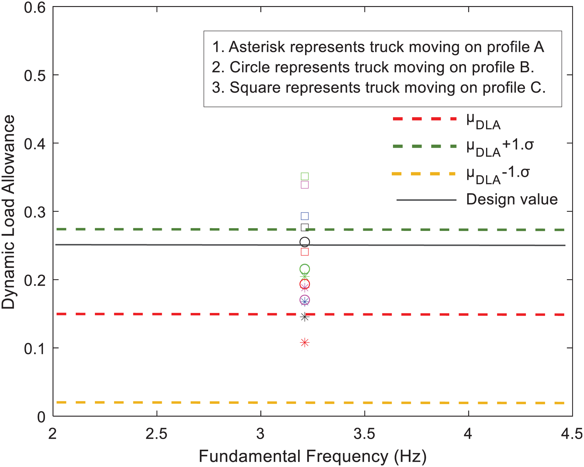
Next, a parametric study was performed for a total of 105 cases using the 3-D finite element model of a bridge generated in Abaqus to determine the effects of speed, spacing, number of trucks in platoons, and the level of pavement surface roughness profiles on the DLA. The value of 0.25 was compared with the DLA for two-truck and three-truck platoons and the three ISO 8608 roughness profiles, as shown in Figures 13 and 14. The DLA was above 0.25 for 13 of 35 configurations with roughness profile A. The DLA was above 0.25 for 18 of 35 cases with roughness profile B, while the DLA was above 0.25 for 30 of 35 cases with roughness profile C. However, the latter is considered exceptionally large for bridges and would probably give rise to speed limitations and therefore smaller DLA. Furthermore, the 0.25 DLA given in Table 1 for multiple axles is calibrated for a CoV of 80%, which accounts for the uncertainty on this value for bridges. Using a DLA of 0.25 and a bias coefficient of 0.6 given in Table C14.3 in CHBDC S6 indicate a mean DLA ( $μ_{DLA}$ ) of 0.15 but with a high CoV of 80%. This results in a standard deviation ( $σ$ ) of 12%. The DLA for the $μ_{DLA} - 1 . σ$ is 3% and the $μ_{DLA} + 1 . σ$ is 27%. This range certainly envelopes the DLA range shown in Figures 12 to 14 for various single and platooning trucks configurations.

In Equation 7, the DLA for a single truck was used as a reference to evaluate the relative effect of platooning trucks on DLA.

Relative difference = \frac{DL A_{platoon}}{DL A_{single truck}}

(7)

Effect of Speed and Inter-Truck Spacing

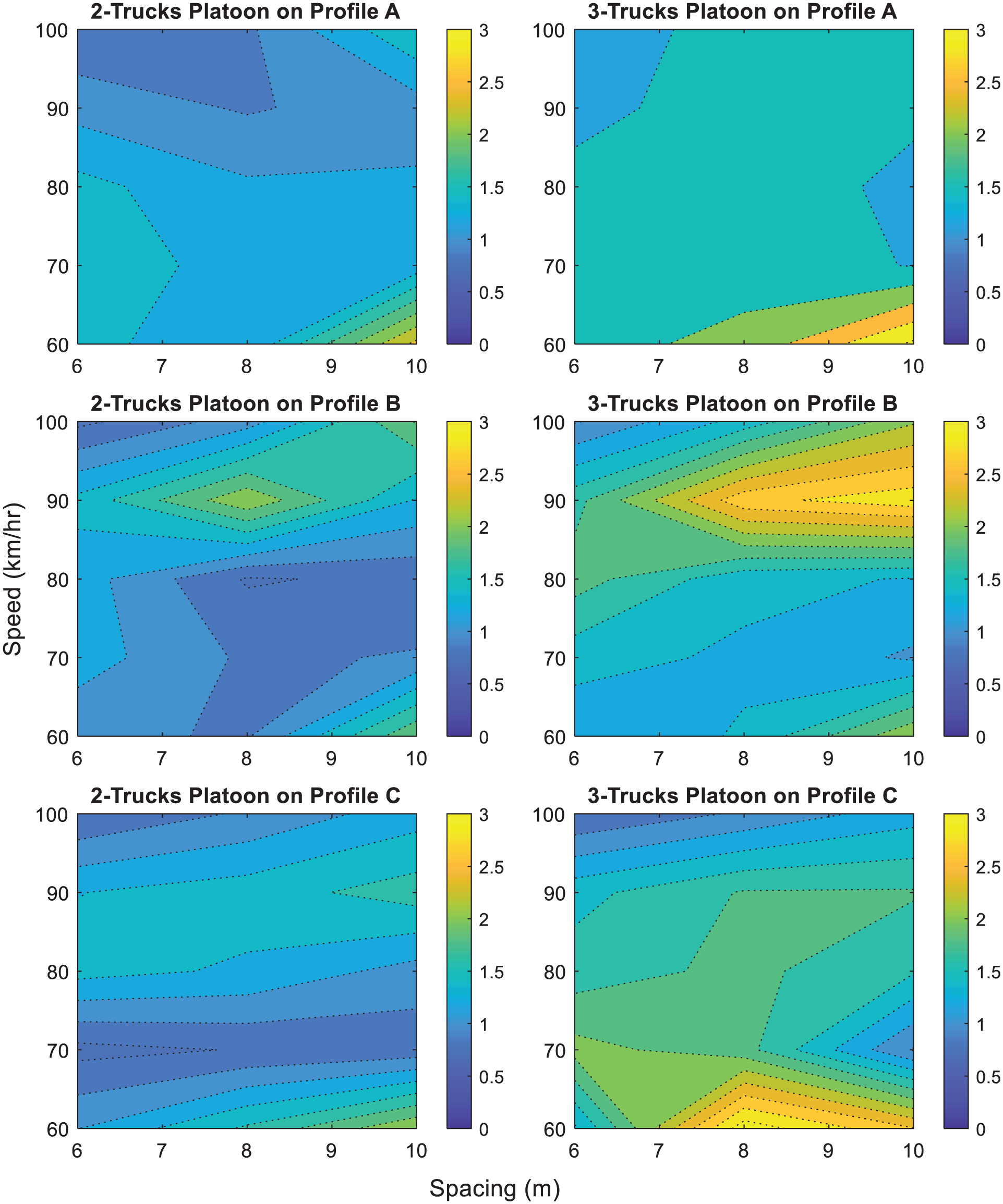
As indicated in Figure 9, speeds ranging from 60 to 100 km/h were considered in this study for all platoon configurations and surface roughness classes. The results indicate that the DLA does not always increase monotonically with increasing speed and decreasing inter-truck spacing. This behavior is attributed to resonance effects that depend both on truck spacing and speed, and the natural frequencies of the bridge ( 30 ). The roughness of the surface profile is also shown to be a contributing factor to the resonance of the bridge. For instance, in Figure 15, the DLA for the same platoon configurations for different surface profiles are shown on the left-hand column of figures as a function of the speed and spacing. It can be seen that the resonance occurs at different speeds and inter-truck spacings for the selected ranges for different roughness profiles. For instance, the highest DLA for a two-truck platoon resulting from resonance effects are observed at 80 km/h and 6 m inter-truck spacing on surface roughness profile A. However, on surface roughness profile B, the highest DLA resulting from resonance occurs at 100 km/h and 10 m inter-truck spacing for the same two-truck platoon. Similarly on surface roughness profile C, the highest DLA resulting from resonance occurs at 90 km/h and 10 m inter-truck spacing for the same two-truck platoon. These observations can be made from Figure 15. The same can be observed for three-trucks platoon configurations on various profiles (Figure 15). For the three-truck platoon configuration, the maximum DLA occurs at 60 km/h and 10 m inter-truck spacing on profile A. However, on surface roughness profile B, the maximum DLA resulting from resonance occurs at 100 km/h and 10 m inter-truck spacing for the three-truck platoon configuration. Similarly on surface roughness profile C, the maximum DLA for the same three-truck platoon occurs at 60 km/h and 8 m inter-truck spacing configuration. The maximum DLA obtained for roughness profile C occurs for a three-truck platoon, inter-truck spacing of 8 m, and 60 km/h (Figures 15 and 16). In some instances, the DLA for platoons is also observed to be smaller than that for the single truck as shown in Figure 16. This occurs for smooth profiles (A and B) for both two- and three-truck platoons but with no specific trend. These observations are consistent with previous results that show a decrease in DLA with an increase in the total static load in the absence of resonance ( 14 ). It can also be observed generally from Figure 16 that lower DLAs relative to a single truck are observed for all the cases studied for ATP moving at 100 km/h at 6-m inter-truck spacing. Similarly, the inter-truck spacing seems to directly influence the DLAs as can be observed for most of the cases of 10-m inter-truck spacing (Figures 15 and 16). The upper limit of inter-truck spacing selected in this study is kept as 10 m as larger spacings can result in higher air-drag which will diminish the fuel savings in platooning. These findings are consistent with Ling et al. ( 32 ) which also suggest that increasing the inter-truck spacing may not be a solution to reduce DLA from platooning loads.

Figure 15.

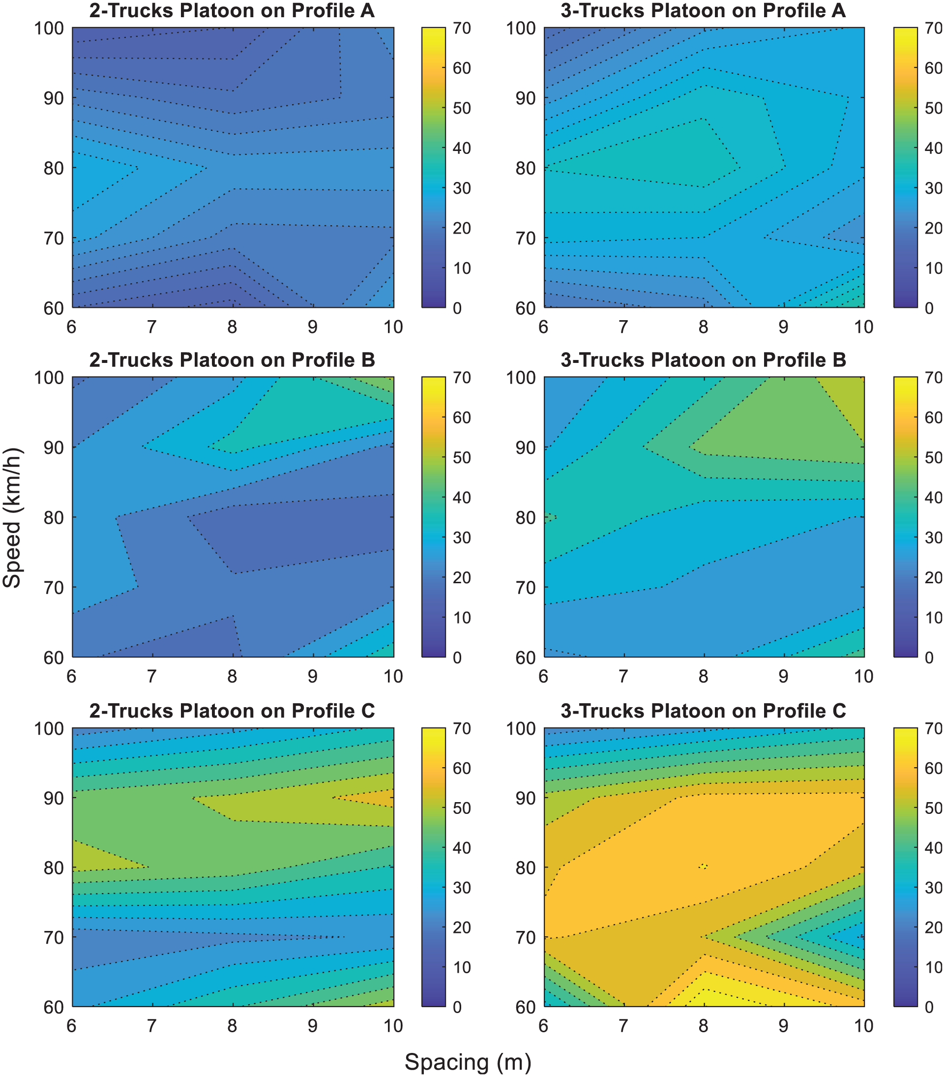
Effect of platoon speed and inter-truck spacing on DLA. The legend represents the DLA in percentage terms.

Figure 16.

Ratio of DLA of different platooning configurations relative to DLA for a single truck as a function of speed and inter-truck spacing.

Consistent relationships are not always observed because of resonance effects between the dynamic platoon loads and the natural frequencies of the bridge. Smaller spacings could also result in the presence of more axles simultaneously on the bridge, which could result in exceeding the loading limits of the bridge ( 57 ). Karbasi et al. ( 58 ) demonstrated that smaller headway spacings can increase the load demand above the capacity of the bridge at any speed.

The number of trucks in a platoon also seems to have a strong influence on DLA, especially for roughness profiles B and C. A higher number of trucks is not an issue from a static load perspective since the bridge span is smaller than the total length of the platoon; however, platoons that are longer than the length of the bridge generate dynamic loads over longer periods of time, which can result in higher DLA as evidenced for three-truck platoons and the roughness profile C (Figures 15 and 16). This issue could not be addressed in the current paper but should be further investigated.25663155902528(a)(a)

Effect of Pavement Surface Roughness

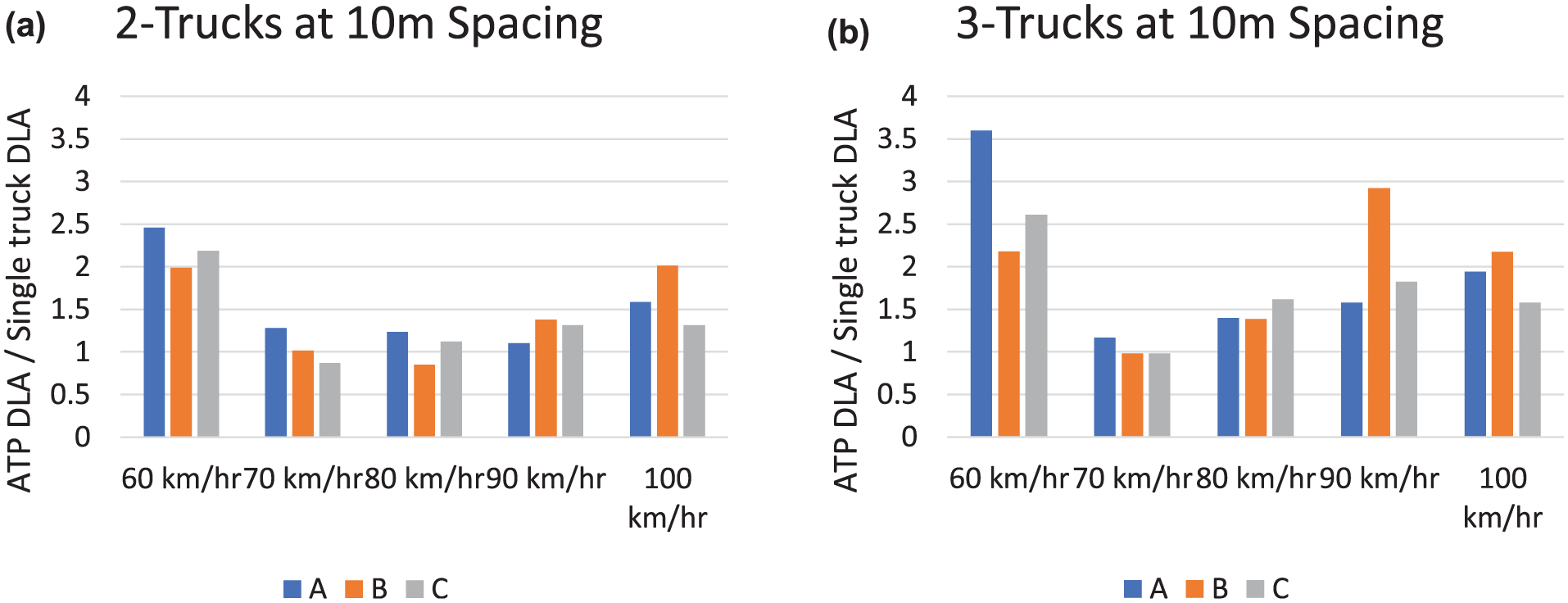
The pavement surface roughness is generally expected to directly increase the DLA, especially when resonance occurs (Figures 11 and 17). The speed at which resonance occurs varies as a function of surface roughness. For example, resonance occurred at 80 km/h for roughness profile A for all platoon configurations except inter-truck spacings greater than 8 m for both two-truck and three-truck platoons. However, different platoon configurations have attained maximum DLAs as a result of resonance conditions at different surface roughness profiles. It is worth noting that the statistics given in Table 14.3C in CHBDC are generally consistent with the limits of mean and standard deviation given in Figure 17 for the various platooning arrangements and single trucks on relatively smoother surfaces (ISO Class A and Class B surface roughnesses). Figures 18 to 20 illustrate the ratio of platoon to single-truck DLA caused by surface roughness for the various combinations of truck platoons investigated. For two-truck platoons with inter-truck spacing of 6 m, the ratio was less than one at 100 km/h for all three surface roughness profiles. A similar trend was observed for almost half of the two-truck configurations on profile B and a few configurations for profile A. There were only a few three-truck configurations (6-m spacing at 100 km/h on profile B, and 10-m at 70 km/h on profiles B and C) where the DLA ratio was less than one.

Figure 17.

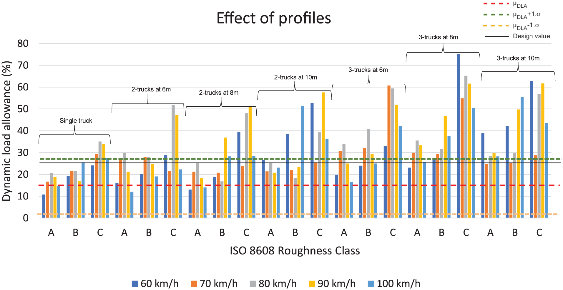
Effect of surface roughness profile on the DLA for different platoon configurations and speeds. The legend represents the DLA in percentage terms.

Figure 18.

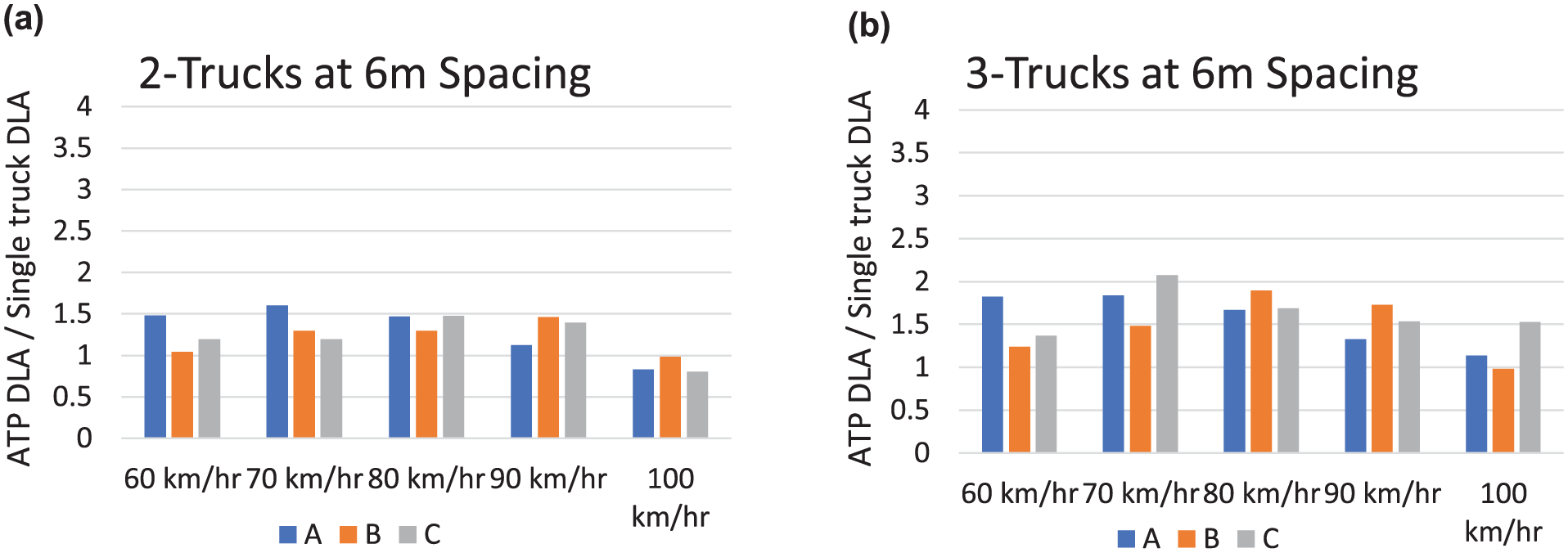
Effect of speed and surface roughness of profile of: (a) two-truck platoon; and (b) three-truck platoon with 6-m inter-truck spacing on the DLA ratio of the respective platoon and that of the single truck. The legend represents the DLA in percentage terms.

Figure 19.

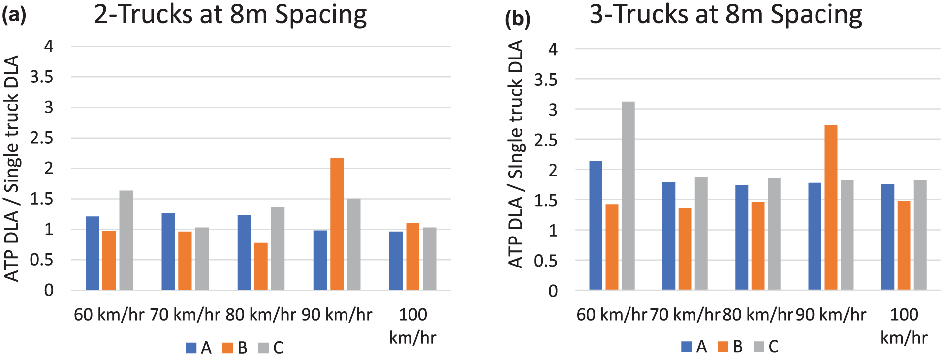
Effect of speed and surface roughness of profile of: (a) two-truck platoon: and (b) three-truck platoon with 8-m inter-truck spacing on the DLA ratio of the respective platoon and that of the single truck. The legend represents the DLA in percentage terms.

Figure 20.

Effect of speed and surface roughness of profile of: (a) two-truck platoon; (b) three-truck platoon with 10-m inter-truck spacing on the DLA ratio of the respective platoon and that of the single truck. The legend represents the DLA in percentage terms.

Concluding Remarks

Autonomous truck platooning is being considered as a cost-saving strategy by the trucking industry; however, the capacity of existing bridges to accommodate this new technology has not been fully investigated.

This paper is aimed at the understanding the dynamic effects of the ATP on a single span steel girder concrete composite bridge. The parameters investigated in the study were the number of trucks (two or three), the inter-truck spacing (6 to 10 m), the speed (60 to 100 km/h) of the ATP, and ISO 8608 road surface roughness profiles (A, B, and C). The bridge geometry, span length, girder spacing, and typology were constant for all the analyses. A computational model of a bridge is used for parametric analysis similar to other published studies. The surface roughness profiles were randomly generated profiles using a PSD approach and subsequently implemented in Abaqus on the bridge deck. The surface roughness profiles generated using PSD were single random realization for each corresponding class (the randomness being introduced by the phase angle) instead of a suite surface roughness generated for each profile. The main conclusions drawn after the analysis pertaining to the selected bridge case are as follows:

a. It was observed that resonance is the governing factor in higher DLA for a given ATP configuration on the bridge, which is a function of surface roughness, platoon configuration, bridge characteristics, and ATP speed.

b. For the ISO 8608 surface roughness Class A, most of the selected ATP configurations result in DLA that are within the current limit specified in CSA S6 for the bridge considered in the article.

c. For the ATP with two or three trucks, the DLA is lower than the DLA for a single truck when the platoon configuration does not enter into resonance with the bridge.

d. An increase in the number of trucks in a platoon with large inter-truck spacing can correspond to resonance conditions that result in higher DLA.

e. Higher speeds for two-truck platoons with close spacing results only in a marginal increase of DLA compared with that of a single truck on rougher surfaces and can result in smaller DLAs than a single truck on smooth profiles.

f. A larger number of trucks in ATP at low speeds and over rough surfaces is conducive to resonance conditions and higher DLA.

Recommendations for Future Work

On the basis of these findings, the following recommendations are suggested as further research to develop comprehensive recommendations:

a. The effect of multiple presence on the DLA should be investigated by simulating other vehicles moving alongside the platooning trucks.

b. More cases should be analyzed to have a sufficiently large sample to perform statistical analyses and formulate recommendations for DLA.

c. Several trucks for platoon lengths greater than the length of the bridge (> 3) should be considered since dynamic effects could be more severe because of the longer duration of dynamic loads.

d. The truck suspension systems stiffness and damping should be further investigated given their influence on the DLA.

e. The investigation should be expanded to bridges with different span lengths, girder spacing, and to continuous bridges with multiple spans. Similarly, other bridge types should also be investigated.

f. Given the significant influence of the pavement surface roughness on DLA, it is recommended to have a survey of the surface roughness of existing pavements on the bridge to quantify the consistency of the surface roughness and the prevalent surface roughness categories.

g. Field studies should be performed on existing bridges as test cases.

Footnotes

Acknowledgements

The authors acknowledge the time and valuable input of the oversight committee members for this project: Alex Au (Ministry of Transportation Ontario), Darrel Gagnon (COWI North America Ltd.), Frédéric Legeron (Parsons Corporation), Majid-Reza Irfani (Ministère des Transports, de la Mobilité durable et de l’Électrification des transports, Quebec), Matthew Sjaarda (WSP Canada), Rosio Morales Rayas (CSA Inc.), and Mark Braiter (CSA Inc.).

Author Contributions

The authors confirm contribution to the paper as follows: study conception and design: Study conception and design: Sikandar Sajid and Luc Chouinard, Finite element modeling and data collection: Sikandar Sajid, and Aizaz Ahmad: analysis, interpretation of results: Sikandar Sajid. and Luc Chouinard; Draft Manuscript preparation and review: Sikandar Sajid and Luc Chouinard. All authors reviewed the results and approved the final version of the manuscript.

Declaration of Conflicting Interests

The authors declared no potential conflicts of interest with respect to the research, authorship, and/or publication of this article.

Funding

The authors disclosed receipt of the following financial support for the research, authorship, and/or publication of this article: This study was supported by the Canadian Standards Association Inc. Toronto, Ontario, Canada.

ORCID iD

Sikandar H. Sajid

References

Bhoopalam

A. K.

Agatz

Zuidwijk

Planning of Truck Platoons: A Literature Review and Directions for Future Research. Transportation Research Part B: Methodological, Vol. 107, 2018, pp. 212–228.

Tsugawa

Kato

Aoki

An Automated Truck Platoon for Energy Saving. In 2011 IEEE/RSJ International Conference on Intelligent Robots and Systems. IEEE, 2011. https://ieeexplore.ieee.org/document/6094549

McAuliffe

Lammert

X. Y

Shladover

Surcel

M. D.

Kailas

Influences on Energy Savings of Heavy Trucks Using Cooperative Adaptive Cruise Control. SAE Technical Paper 2018-01-1181, 2018.

Zhang

Peng

Zhao

Can Autonomous Vehicles Save Fuel? Findings from Field Experiments. Journal of Advanced Transportation, Vol. 2022, 2022.

Bureau-of-Transportation-Statistics. 2017 CFS Preliminary Data. U.S. Department of Transportation, 2018December. https://www.bts.gov/surveys/commodity-flow-survey/2017-cfs-preliminary-data.

Van Arem

Van Driel

C. J.

Visser

The Impact of Cooperative Adaptive Cruise Control on Traffic-Flow Characteristics. IEEE Transactions on Intelligent Transportation Systems, Vol. 7, No. 4, 2006, pp. 429–436.

Lioris

Pedarsani

Tascikaraoglu

F. Y.

Varaiya

Platoons of Connected Vehicles Can Double Throughput in Urban Roads. Transportation Research Part C: Emerging Technologies, Vol. 77, 2017, pp. 292–305.

Alsghan

Chitturi

M. V.

Noyce

D. A.

Road Sign Occlusion Under Truck Platooning. Journal of Transportation Engineering, Part A: Systems, 147, No. 9, 2021, p. 04021045.

Lee

Impact of Automated Truck Platooning on the Performance of Freeway Mixed Traffic Flow. Journal of Advanced Transportation, Vol. 2021, 2021.

10.

Rana

M. M.

Effect of Autonomous Vehicles on Pavement Distress & Road Safety and Pavement Distress Optimization. M.Eng. thesis. Memorial University of Newfoundland, 2021.

11.

Oleson

Scott

Schumacher

Unnikrishnan

Zhu

Impact of Truck Platooning on Loading of Bridges in Oregon. Oregon Department of Transportation, Research Section, 2024.

12.

Sajid

Chouinard

Legeron

Ude

Ajrab

Reliability Analysis of Bridges for Autonomous Truck Platoons. Transportation Research Record, Vol. 2677, No. 1, 2023, pp. 1071–1081.

13.

AASHTO-LRFD. Bridge Design Specifications, 8th ed. American Association of State Highway and Transportation Officials, Washington, D.C., 2017.

14.

Nowak

A. S.

Calibration of LRFD Bridge Design Code, NCHRP Report 368. Transportation Research Board, Washington, D.C., 1999, pp. 9–28.

15.

Lutomirska

Live Load Models for Long Span Bridges. MS thesis. Civil Engineering, University of Nebraska – Lincoln, 2009, p. 1.

16.

Hwang

E.-S.

Nowak

A. S.

Simulation of Dynamic Load for Bridges. Journal of Structural Engineering, Vol. 117, No. 5, 1991, pp. 1413–1434.

17.

Sayed

S. M.

Sunna

H. N.

Moore

P. R.

Truck Platooning Impact on Bridge Preservation. Journal of Performance of Constructed Facilities, Vol. 34, No. 3, 2020, p. 04020029.

18.

Sajid

Chouinard

Carino

Condition Assessment of Concrete Plates Using Impulse-Response Test with Affinity Propagation and Homoscedasticity. Mechanical Systems and Signal Processing, Vol. 178, 2022, p. 109289.

19.

Tohme

Yarnold

Steel Bridge Load Rating Impacts Owing to Autonomous Truck Platoons. Transportation Research Record, Vol. 2674, No. 2, 2020, pp. 57–67.

20.

Yarnold

M. T.

Weidner

J. S.

Truck Platoon Impacts on Steel Girder Bridges. Journal of Bridge Engineering, Vol. 24, No. 7, 2019, p. 06019003.

21.

Couto Braguim

Lou

Nassif

Truck Platooning to Minimize Load-Induced Fatigue in Steel Girder Bridges. Transportation Research Record, Vol. 2675, No. 4, 2020, p. 0361198120973657.

22.

Ling

Deng

Load Effect of Automated Truck Platooning on Highway Bridges and Loading Strategy. Sensors, Vol. 22, No. 20, 2022, p. 7704.

23.

AASHTO. The Manual for Bridge Evaluation, 3rd ed. AASHTO, Washington, D.C., 2018.

24.

Elshazli

M. T.

Ibrahim

Abdel-Rahim

Truck Platooning Impact on Existing Bridges’ Load Ratings. Journal of Structures, Vol. 51, 2023, pp. 1706–1721.

25.

Elshazli

Ahmed

A.-R.

Impact of Autonomous and Connected Truck Platoons in the Pacific Northwest on Transportation Infrastructure. Pacific Northwest Transportation Consortium (PacTrans) (UTC), University of Washington, 2022.

26.

Thulaseedharan

N. P.

Yarnold

M. T.

Prioritization of Texas Prestressed Concrete Bridges for Future Truck Platoon Loading. Bridge Structures, Vol. 16, No. 4, 2020, pp. 155–167.

27.

Wassef

Truck Platooning Impacts on Bridges: Phase I – Structural Safety, FHWA-HIF-21-043. FHWA, Washington, D.C., 2021July.

28.

Yang

Steelman

J. S.

Puckett

J. A.

Linzell

D. G.

Safe Platooning Headways on Girder Bridges. Transportation Research Record, Vol. 2679, No. 1, 2021, p. 03611981211036379.

29.

Steelman

J. S.

Puckett

J. A.

Linzell

D. G.

Yang

Truck Platooning Effects on Girder Bridges. Nebraska Department of Transportation, Lincoln, 2021.

30.

Braley

J. B.

Understanding Vehicle-Bridge Interaction Through Field Measurements and Model-Based Simulations. Rutgers The State University of New Jersey, School of Graduate Studies, 2019.

31.

CHBDC. Canadian Highway Bridge Design Code. Canadian Standards Association, Ottawa, ON, Canada, 2019.

32.

Ling

Cao

Deng

Zhong

Dynamic Impact of Automated Truck Platooning on Highway Bridges. Engineering Structures, Vol. 262, 2022, p. 114326.

33.

Ling

Deng

Cao

Zhong

Determination of Dynamic Amplification Factors for Small-and Medium-Span Highway Bridges Considering the Effect of Automated Truck Platooning Loads. Mechanical Systems and Signal Processing, Vol. 204, 2023, p. 110812.

34.

Tilly

Dynamic Behaviour of Concrete Structures Report of the RILEM 65-MDB Committee. Materials and Structures, Vol. 19, 1986, p. 460.

35.

Paultre

Chaallal

Proulx

Bridge Dynamics and Dynamic Amplification Factors—A Review of Analytical and Experimental Findings. Canadian Journal of Civil Engineering, Vol. 19, No. 2, 1992, pp. 260–278.

36.

AASHTO

ed.

Standard Specifications for Highway Bridge Design, 17th ed. Washington, D.C., 2002.

37.

BSI. 1À2 Eurocode 1. Actions on Structures–Part 2: Traffic Loads on Bridges. British Standards Institution, Management Centre: rue de Stassart, 36 B-1050 Brussels, 1991.

38.

Deng

Zou

Cai

C. S.

State-of-the-Art Review of Dynamic Impact Factors of Highway Bridges. Journal of Bridge Engineering, Vol. 20, No. 5, 2015, p. 04014080.

39.

Nowak

A. S.

Lutomirska

Sheikh Ibrahim

The Development of Live Load for Long Span Bridges. Bridge Structures, Vol. 6, No. 1–2, 2010, pp. 73–79.

40.

Gao

Reliability-Based Evaluation of Bridges Live Load Carrying Capacity in the United States. Estados Unidos, Washington, D.C., 2012.

41.

Yang

Y.-B.

Yau

J.-D.

Vehicle-Bridge Interaction Element for Dynamic Analysis. Journal of Structural Engineering, Vol. 123, No. 11, 1997, pp. 1512–1518.

42.

Chang

Yang

Disk Model for Wheels Moving Over Highway Bridges with Rough Surfaces. Journal of Sound and Vibration, Vol. 330, No. 20, 2011, pp. 4930–4944.

43.

Afia

A. B.

Annan

C.-D.

Dey

Dynamic Behavior of Aluminum Deck-on-Steel Girders Bridges under Vehicular Loads Considering the Effect of Road Roughness. In Presented at IABSE Congress: Structural Engineering for Future Societal Needs, Ghent, Belgium, 22–24 September2021, pp. 1623–1632. DOI: 10.2749/ghent.2021.1623

44.

Sajid

S. H.

Chouinard

Dynamic Load Allowance for Bridges Subject to Autonomous Truck Platoons. Canadian Standards Association, Toronto, ON, Canada, 2024.

45.

Gao

Zhang

Dai

A Stochastic Quarter-Car Model for Dynamic Analysis of Vehicles with Uncertain Parameters. Vehicle System Dynamics, Vol. 46, No. 12, 2008, pp. 1159–1169.

46.

Tyan

Hong

Y.-F.

S.-H.

Jeng

W. S.

Generation of Random Road Profiles. Journal of Advanced Engineering, Vol. 4, No. 2, 2009, pp. 1373–1378.

47.

Lenkutis

Čerškus

Šešok

Dzedzickis

Bučinskas

Road Surface Profile Synthesis: Assessment of Suitability for Simulation. Symmetry, Vol. 13, No. 1, 2020, p. 68.

48.

Andren

Power Spectral Density Approximations of Longitudinal Road Profiles. International Journal of Vehicle Design, Vol. 40, No. 1–3, 2006, pp. 2–14.

49.

Agostinacchio

Ciampa

Olita

The Vibrations Induced by Surface Irregularities in Road Pavements–A Matlab® Approach. European Transport Research Review, Vol. 6, No. 3, 2014, pp. 267–275.

50.

Technical Committee: ISO/TC 108/SC 2. Mechanical Vibration—Road Surface Profiles—Reporting of Measured Data, Vol. 8608. International Organization for Standardization, 1995. https://www.iso.org/standard/71202.html

51.

Múčka

International Roughness Index Specifications Around the World. Road Materials and Pavement Design, Vol. 18, No. 4, 2017, pp. 929–965.

52.

Loprencipe

Zoccali

Use of Generated Artificial Road Profiles in Road Roughness Evaluation. Journal of Modern Transportation, Vol. 25, 2017, pp. 24–33.

53.

Harris

N. K.

OBrien

E. J.

González

Reduction of Bridge Dynamic Amplification through Adjustment of Vehicle Suspension Damping. Journal of Sound and Vibration, Vol. 302, No. 3, 2007, pp. 471–485.

54.

Green

M. F.

Cebon

Cole

D. J.

Effects of Vehicle Suspension Design on Dynamics of Highway Bridges. Journal of Structural Engineering, Vol. 121, No. 2, 1995, pp. 272–282.

55.

Deng

Cai

Development of Dynamic Impact Factor for Performance Evaluation of Existing Multi-Girder Concrete Bridges. Engineering Structures, Vol. 32, No. 1, 2010, pp. 21–31.

56.

Lim

RufGen: A Plug-in for Rough Surface Generation in Abaqus/CAE. SoftwareX, Vol. 22, 2023, p. 101380.

57.

Steelman

J. S.

Puckett

J. A.

Linzell

D. G.

Yang

Truck Platooning Effects on Girder Bridges: Phase II-Service. Nebraska Department of Transportation, 2023.

58.

Karbasi

A. H.

Budisa

Yang

The Impact of Truck Platooning on Traffic Flow Considering Bridge Safety Index. In 2023 IEEE 26th International Conference on Intelligent Transportation Systems (ITSC). IEEE, 2023.

Dynamic Load Allowance of Bridges Subject to Autonomous Truck Platooning

Abstract

Keywords

Review of Literature on Autonomous Truck Platooning

Dynamic Load Allowance Provisions by Current Design Guidelines

Finite Element Modeling

Truck Load Modeling

Selection of Candidate Truck

Modeling of Truck Loads

Road Surface Roughness Modeling

Generating Road Surface Roughness Profile

Implementation of Road Surface Roughness Profile in Finite Element Tool

Numerical Simulations

Results and Discussion

Effect of Speed and Inter-Truck Spacing

Effect of Pavement Surface Roughness

Concluding Remarks

Recommendations for Future Work

Footnotes

Acknowledgements

Author Contributions

Declaration of Conflicting Interests

Funding

ORCID iD

References