
Abstract
Accurate estimation of traffic state under oversaturated conditions is fundamental to a wide range of transportation applications. While intuitive, volume-to-capacity (
Keywords
Accurate traffic state estimation, including speed, demand, and travel time, is fundamental for transportation planning, operations, and management. Traditional estimation approaches heavily rely on link performance functions (LPFs), such as the widely used Bureau of Public Roads (BPR) function (
1
), which estimate travel time using the volume-to-capacity (
Over the past several decades, numerous forms of LPFs have been developed (
1
–
6
). Among these models, the BPR function has remained the most widely adopted owing to its simplicity and ease of implementation. However, most existing LPFs, including BPR, rely heavily on the volume-to-capacity ratio as the key explanatory variable. While intuitive, this formulation raises several issues when applied to oversaturated traffic conditions, particularly concerning how demand is defined and how the
In particular, bottleneck locations such as intersections, freeway ramps, and lane reductions play a central role in determining network performance ( 7 , 8 ). Accurate quantification of travel demand at these bottlenecks is critical yet challenging owing to physical constraints and latent flow behaviors. Inaccurate or biased demand estimation may introduce substantial errors in traffic state modeling, thereby limiting the effectiveness of congestion mitigation strategies and leading to suboptimal infrastructure or policy decisions. These limitations highlight the need for a more theoretically sound and practically applicable approach, particularly in high-congestion or capacity-constrained environments where accurate estimation of demand and travel time is critical.
Motivation
Building on these challenges, the accurate estimation of bottleneck demand is particularly important for a wide range of transportation planning applications, including infrastructure design, long-term planning, and Transportation Systems Management and Operations (TSMO). In oversaturated regimes, traffic demand often becomes latent and unobservable owing to physical bottlenecks, leading to a decoupling between observed volume and actual demand. This phenomenon introduces systematic bias in travel time estimation, particularly in urban networks and corridor bottleneck characterized by recurrent congestion. Existing classical static or quasi-dynamic models, which estimate demand based on observed volume, tend to underestimate true demand and fail to capture queue spillbacks, delayed vehicle entry, and flow breakdown effects.
Figure 1 illustrates the fundamental interaction between traffic demand and supply and highlights the consequences of incorrect demand inference on traffic state estimation. In Figure 1a, the red demand curve shows an inverse relationship between travel cost (e.g., travel time on the Y-axis) and traveler volume (X-axis). Figure 1b presents the blue supply curve, where increasing volume leads to sharply rising travel cost owing to congestion and capacity constraints. (Color online only.) Figure 1c integrates these curves to identify an equilibrium point (Point B) where demand meets supply. However, when demand is misestimated, such as in oversaturated conditions where latent demand remains unobserved, the equilibrium may shift to a false point (Point A), which underrepresents both flow and travel time. This misinterpretation may result in a significant underestimation of actual demand, thereby distorting traffic state assessment and impairing subsequent planning and management decisions.
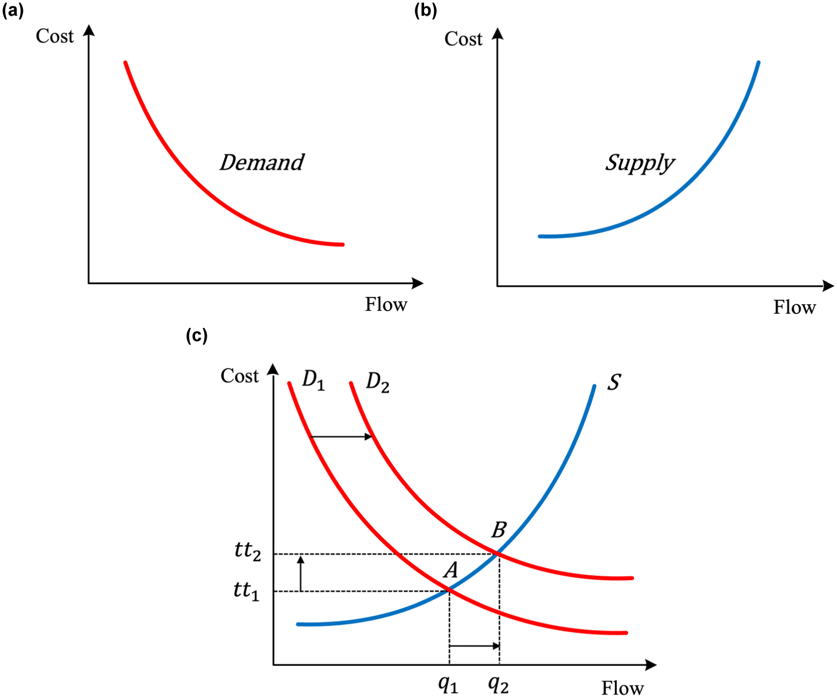
Demand interaction and equilibrium in traffic-flow modeling: (a) Demand curve showing reduced demand as cost increases, (b) Supply curve showing increased cost as flow increases, and (c) Equilibrium point where demand and supply intersect.
A key challenge arises from the inconsistency between empirical traffic patterns and the assumptions underlying conventional LPFs. Detector-based speed-flow plots often display a U-shaped curve: speeds decrease with increasing flow until capacity is reached, followed by simultaneous declines in both speed and flow under oversaturation. However, conventional LPFs such as the BPR function assume a monotonically increasing
Objective and Contributions
This study aims to enhance traffic state estimation under oversaturated conditions by developing a Greenshields-grounded demand inference method capable of capturing latent demand constrained by bottlenecks. A modified demand-delay function is also derived to reflect more accurate congestion dynamics. Together, these models support better-informed decision-making in traffic control, congestion mitigation, and urban mobility management.
This research addresses the limitations of existing demand estimation methods, particularly their inability to account for unobserved demand when the flow is constrained by bottleneck capacity. Two major challenges are targeted: (1) the inability of the volume-to-capacity ratio to represent oversaturated states accurately; and (2) the lack of a practical demand estimation framework within classical traffic flow models like Greenshields model ( 14 ).
The main contributions of this study are summarized as follows:
Improved Demand Estimation Model. An extended Greenshields-grounded traffic flow model is proposed, incorporating a real-time inflow adjustment parameter to estimate latent demand under oversaturated conditions. This model addresses the limitations of the commonly used fundamental diagram (FD)-based symmetric method, which restricts the
Modified LPF. A revised demand-delay function is developed by modifying the classical BPR function to use the demand-to-capacity (
Empirical Validation and Corridor Comparison. The proposed methods are validated using real-world traffic data from two corridors: the West Third Ring in Beijing and the I-405 corridor in Los Angeles. The results confirm that the proposed model significantly improves demand and travel time estimation accuracy, with notable reductions in error metrics compared with benchmark methods. The comparative analysis also reveals differences in congestion dynamics shaped by urban structure.
The remainder of this paper is structured as follows: The second section reviews the related literature. The third section briefly presents the preliminaries that this study is built on. The fourth section presents the proposed methodology. The fifth section describes the case study design and data. The sixth section discusses the numerical analysis results. The seventh section concludes the paper and offers directions for future research.
Literature Review
In a simplified traffic system, where all demand enters upstream of a single congestion point and no other upstream bottlenecks exist, traffic demand at the bottleneck can be estimated by measuring inflow and outflow and accounting for the travel time from the observation point to the bottleneck ( 15 ). However, real-world networks often contain multiple bottlenecks and exhibit congestion propagation upstream ( 16 ). Under such conditions, observed flows within or downstream of the bottleneck do not accurately represent the true traffic demand, especially during oversaturated periods.
Traditionally, traffic demand estimation models are classified into static and dynamic models, based on their ability to capture temporal variation. Static models assume constant demand over time and are widely used for long-term planning. These models rely on historical data, trip generation models, and equilibrium-based traffic assignments. Examples include the Four-Step Travel Demand Model (TDM) ( 17 , 18 ) and volume-delay functions such as the BPR function ( 1 ).
The BPR function and its variants form the foundation of many widely used LPFs. The original formulation was motivated by the practical observability of traffic volume and its intuitive relationship with delay. In particular, the use of the volume-to-capacity ratio as the explanatory variable assumes a monotonic increase in travel time as volume increases, under the assumption that observed volume reflects system demand. This approach has been widely adopted in practice and research owing to the ready availability of volume data from loop detectors, sensors, and traffic counts, especially when direct demand data is unavailable. It also facilitates macroscopic planning and performance assessment in large-scale networks. However, in oversaturated conditions, this assumption breaks down, as traffic volume becomes constrained by capacity and thus no longer represents true demand. This limitation motivates the need to revisit the foundational assumptions of BPR-based models and develop modified formulations that better reflect traffic dynamics under congestion. Several recent studies ( 19 – 21 ) have also emphasized this need.
While effective for macro-level planning, static models fail to capture real-time congestion dynamics such as queue spillbacks and demand surges during peak periods. In contrast, dynamic models consider time-dependent variation in demand and are commonly applied in real-time traffic control, forecasting, and adaptive management. Examples include time-dependent origin–destination (OD) estimation ( 22 – 26 ), dynamic traffic assignment ( 27 ), and machine learning-based approaches. Although dynamic models offer greater flexibility and accuracy, they require substantial real-time data and computational resources. Furthermore, both static and dynamic models often fail to capture excess demand that remains unobservable owing to bottleneck capacity constraints, underscoring the need for improved demand estimation under oversaturated conditions.
One of the most common demand estimation methods relies on observed traffic flow data from loop detectors, automatic counters, or probe vehicles ( 28 , 29 ). These methods assume that observed flow reflects actual demand. However, this assumption breaks down under oversaturated conditions, as observed flow becomes constrained by capacity and no longer scales with demand. Queuing effects further complicate matters: upstream queues can block vehicle entry into the bottleneck segment, and the measured outflow may not reflect total incoming demand. Various correction approaches have been proposed, including backpropagation methods, microscopic simulation, and capacity-constrained models. An alternative and more robust strategy uses traffic density rather than observed flow for demand estimation ( 13 , 30 ). Traffic density is defined as the number of vehicles per unit distance and serves as a key variable in flow theory (e.g., the Greenshields model). Unlike flow, it remains elevated under oversaturated conditions, providing a more reliable indicator of congestion intensity and latent demand.
Several classical and contemporary studies have advanced bottleneck demand estimation. May ( 28 ) introduced the “excess density” method to estimate demand at isolated bottlenecks. Building on this, Jia et al. ( 31 ) applied log-normal fitting to multi-day demand distributions and introduced an autoregressive error model. Huntsinger and Rouphail ( 10 ) estimated bottleneck demand by incorporating queuing effects at signalized intersections into the capacity constraint. Small and Verhoef ( 32 ) proposed a piecewise linear approach for hyper-congestion demand, framing it as “inflow demand” shaped by capacity and queuing. Newell ( 33 ) developed a polynomial-based model linking arrival rates and dissipation flows to estimate demand. Cheng et al. ( 34 ) further extended Newell’s model by refining the polynomial demand formulation for oversaturated conditions.
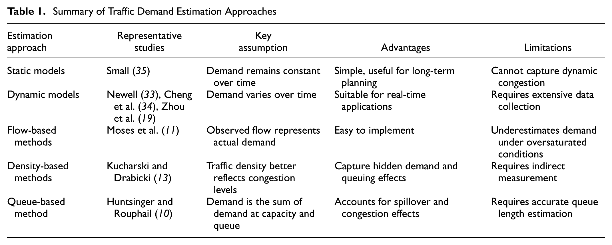
In summary, traffic demand estimation methods vary in their assumptions, data requirements, and performance. Static models offer long-term insights but fail under dynamic congestion. Dynamic models adapt to time-varying demand but require rich data inputs. Flow-based methods are easy to implement but underestimate demand in oversaturated conditions. Density-based approaches provide better accuracy by capturing latent, unobservable demand. Table 1 summarizes the main categories and their characteristics.
Summary of Traffic Demand Estimation Approaches
Preliminaries
This section introduces the foundational concepts that this study builds on, focusing on traffic dynamics under oversaturated conditions and the baseline demand inference method used for comparison. In particular, we present system characteristics relevant to travel delay and congestion at bottlenecks, followed by the introduction of the symmetric method for estimating traffic demand under oversaturated conditions ( 11 , 20 , 21 ).
Characteristics of Traffic Flow Under Oversaturated Conditions
From an analytical modeling perspective, traffic flow through bottlenecks exhibits distinct dynamics during congestion, including oversaturated flow, increasing delay, prolonged travel times, capacity drops, and delayed recovery. These phenomena reduce throughput at bottleneck locations and can lead to upstream congestion propagation, significantly affecting overall network performance. When traffic flow encounters a bottleneck, capacity limitations reduce vehicle speeds below the critical threshold
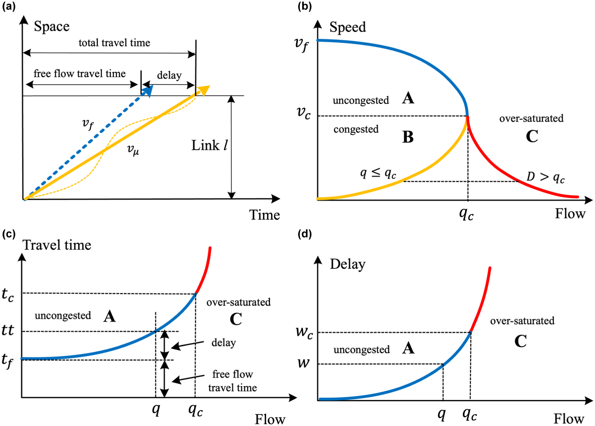
Illustration of traffic flow characteristic in a bottleneck: (a) space-time vehicle trajectory in a bottleneck; (b) speed-flow and demand relationship; (c) flow and travel time relationship; (d) flow and delay relationship. Color online only.
Figure 2a illustrates vehicle trajectories through a bottleneck segment from a space-time perspective. As vehicles traverse the bottleneck of length

The relationship between speed and flow is illustrated in Figure 2b by blue and yellow curves, which represent Regions A and B, respectively. (Color online only.) The upper part Region A represents the uncongested regime, where vehicles primarily travel at free-flow speed
However, as traffic density continues to rise and approaches the critical density
In uncongested conditions, referred to as Region A, the observed flow typically reflects the true demand. However, in the congested regime, referred to as Region C, the actual demand often exceeds the bottleneck capacity. This excess demand cannot be captured by observed flow owing to capacity constraints. As a result, conventional traffic data from detectors significantly underestimates the true demand in Region C. To address this issue, it becomes necessary to apply alternative estimation strategies that can infer latent demand from observed traffic states. The symmetric method serves as one such approach by conceptually reflecting flow values across the capacity threshold, thereby approximating the level of unserved demand during periods of severe congestion.
Figure 2, c and
d
, depicts the relationships between flow and travel time, and flow and delay, respectively. In Figure 2c, travel time increases gradually as flow approaches capacity. Once flow exceeds
In the next section, we introduce the symmetric method ( 11 , 20 , 21 ), which attempts to infer the unobservable traffic demand during oversaturated periods (Region C of Figure 2b) by estimating latent flow not captured by conventional sensors.
Deriving Traffic Demand Using the Symmetric Method
Key Parameters for Demand–Supply Interaction
Accurately estimating traffic demand is critical for understanding bottleneck congestion, as it reflects the extent to which flow is constrained by roadway capacity. From a macroscopic perspective, demand is treated as a static quantity, whereas at the mesoscopic level, it evolves dynamically with traffic conditions. This subsection identifies and ranks key parameters influencing bottleneck demand estimation to improve the characterization of demand–supply interactions under oversaturated conditions.
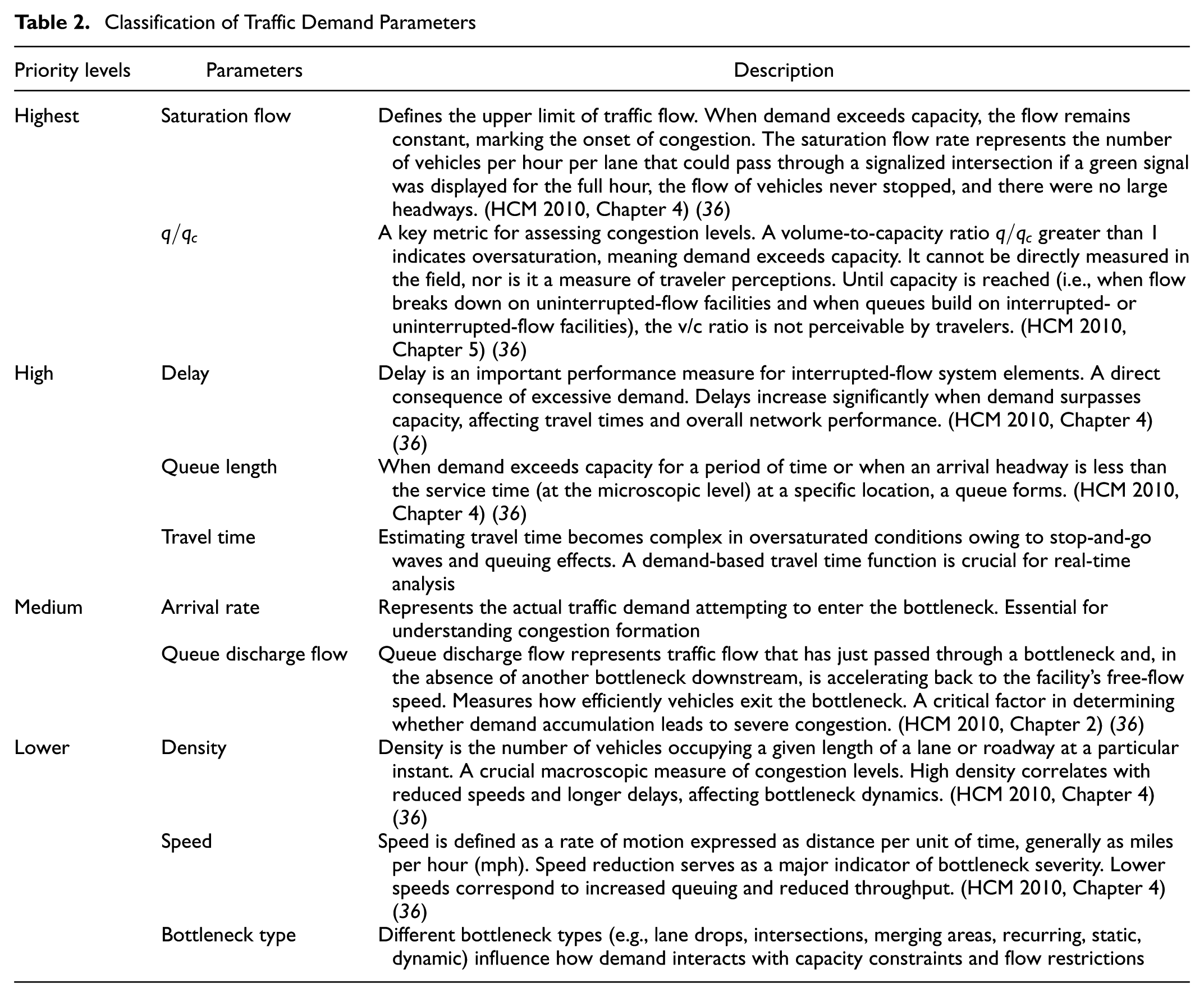
Traffic demand parameters can be grouped by their direct influence on bottleneck formation, congestion propagation, and traffic performance. Saturation flow is one of the key factors in determining the operational capacity of signalized intersections, whereas indicators such as the
Classification of Traffic Demand Parameters
Capacity Adjustment Via the Symmetric Method
Traffic demand can be defined as the sum of vehicles that successfully traverse a segment and those that are queued but intend to pass during the observation period. Accordingly, the total demand D at a bottleneck is given by:
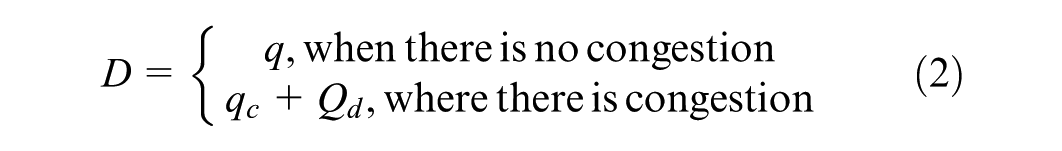
where
The symmetric method (
11
,
20
,
21
), used in this study as a baseline for estimating latent demand under oversaturated conditions, is grounded in the FD of traffic flow. It assumes a mirrored relationship between speed and flow across the capacity threshold
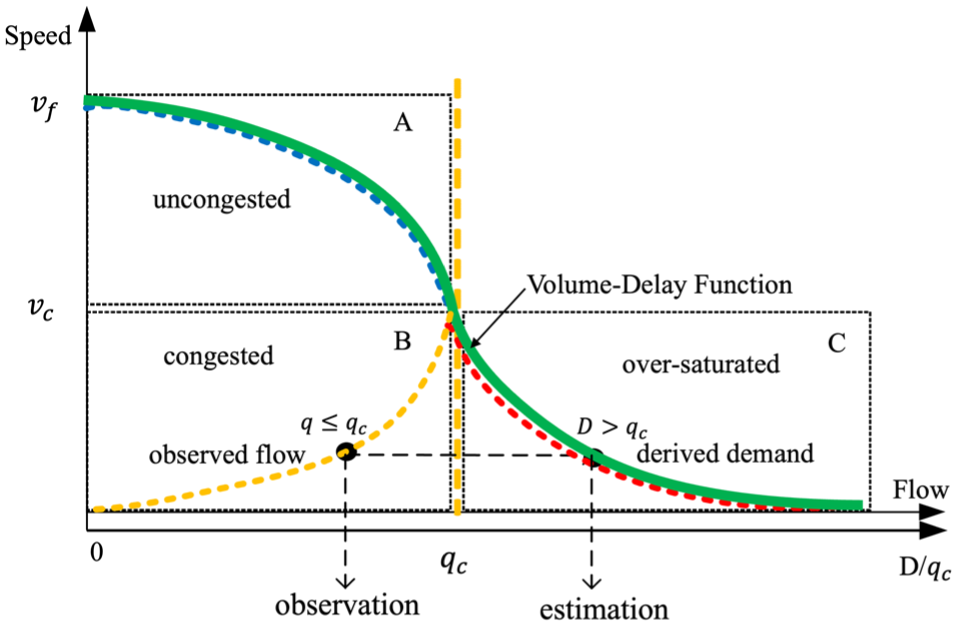
Mapping the demand with the observed flow based on the symmetric method.
The estimated demand of the symmetric method is calculated as:

From Equations 2 and 3, the number of queued vehicles can be expressed as:

Equation 3 leads to the following theoretical range of the

However, under extreme or non-recurrent congestion scenarios such as peak hour, special events, or adverse weather conditions, actual demand may cause
This method is derived directly from the FD and provides a smooth transition between free-flow and oversaturated conditions. Its simplicity makes it suitable for real-time and short-term demand estimation at bottlenecks. However, it does not account for long-term queue accumulation and assumes that queuing dissipates rapidly.
Time-Accumulated Method for Traffic Demand Estimation
From the observational perspective, traffic demand

where
Figure 4 illustrates this method. During congestion, flow decreases and later recovers as traffic clears. This method accumulates flow over time to capture both instantaneous and latent demand, including vehicles delayed but still intending to pass through the bottleneck.
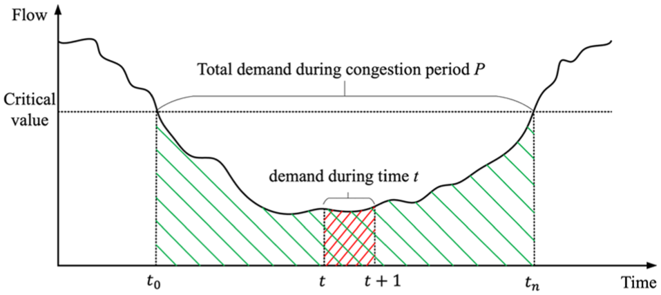
Illustration of the time-accumulated method for demand estimation during congestion conditions.
The time-accumulated method is effective for evaluating peak-hour conditions and long-term congestion patterns. Unlike point-in-time approaches, it reflects the total demand over the entire congested period. This provides a more comprehensive view of system performance and is particularly useful for predicting queue length, as the gap between cumulative demand and throughput indicates potential queue growth.
However, this method is more computationally intensive, requiring detailed time-series data across extended periods. Its accuracy also depends heavily on identifying congestion time boundaries
Methodology
The symmetric method introduced in Equation 3 serves as a useful baseline for estimating traffic demand under oversaturated conditions. However, it tends to systematically underestimate actual demand owing to several inherent limitations. First, bottleneck flow constraints restrict the observed flow
This section introduces a methodological enhancement to improve the estimation accuracy of traffic demand under oversaturated conditions using the symmetric method.
Extending the Greenshields Model for Improved Traffic Demand Estimation
We introduce a correction factor to capture unobserved latent demand. The correction is derived by leveraging the Greenshields model ( 14 ), which offers a theoretically grounded and empirically validated framework for modeling traffic flow at the macroscopic level.
The corrected demand estimation model proposed in this paper is formulated as follows:

where
In the Greenshields model, the relationship between flow
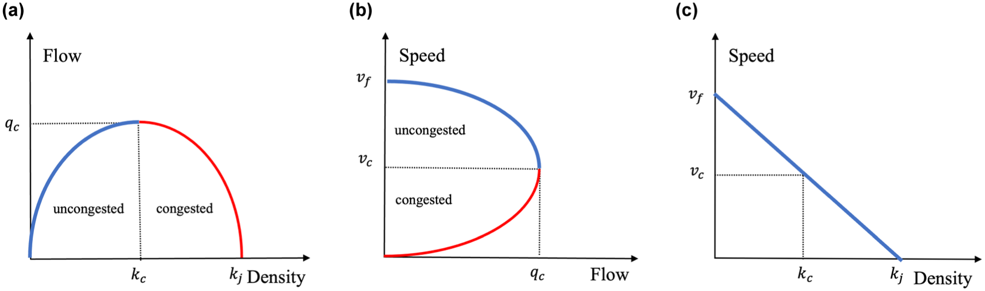
The fundamental diagram (FD) in Greenshields model: (a) flow–density relationship; (b) speed–flow relationship; (c) speed–density relationship.
The mathematic relationships between speed–density and flow–density of the Greenshields model can be utilized as a basis for consistency correction. The equations are given as follows:


According to the Greenshields model, under oversaturated conditions (

Solving for

Thus, the maximum flow occurs at:
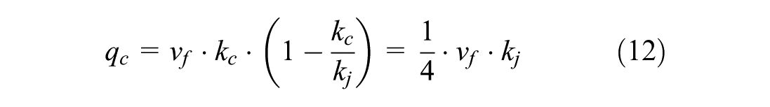
Equation 10 represents the rate of change of flow with density, which in turn affects the unobserved demand component. When density increases beyond

A larger
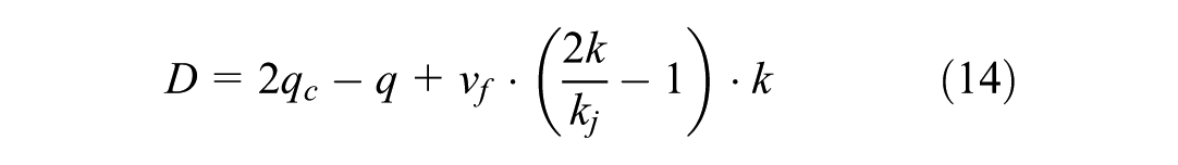
The final corrected demand estimation formula is given as follows:
The behavior of correction factor
(1) When traffic density is low (
(2) When traffic density approaches the critical density (
(3) When traffic density is high (
Specifically, to accurately estimate traffic demand at bottleneck locations, we propose the following solution process.
(1) First, we calibrate Greenshields model parameters by calibrating
(2) Next, we compute the observed flow
(3) Finally, we estimate travel time and perform adjustments by comparing the results with actual observed data.
The

This implies that
Mapping the demand with the observed flow based on the symmetric method.
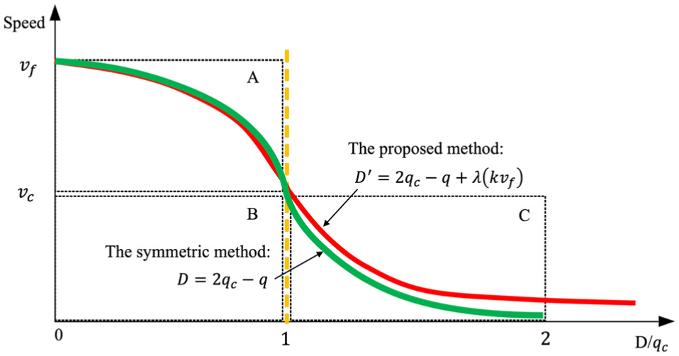
Using the Greenshields-grounded modified demand formulation in Equation 14, the resulting
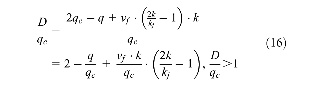
When
Therefore, the proposed modified approach addresses the limitations of the traditional symmetric method ( 11 , 20 , 21 ), providing improved estimation accuracy across varying levels of resolution and enhanced applicability under both typical and extreme congestion conditions.
Derivation of Travel Time Estimation Model
In most papers related to LPFs, researchers have primarily focused on the BPR function in its polynomial form, as it efficiently and simply relates traffic volume to delays, making it widely used in transport planning software. However, it also presents certain inherent challenges (
37
–
39
). The calibrated function may exhibit a non-negligible error when applied to congestion conditions, such as bottleneck. Additionally, the BPR function fails to capture traffic flow dynamics and queue evolution processes (
40
), which limits its accuracy and applicability in describing oversaturated bottlenecks characterized by high density but low throughput. Therefore, in this section, we use the BPR function as a benchmark and modify its key parameter,
The classical BPR function is formulated as follows:

where
Within traffic flow analysis, the
Typically,
In this study, the

By substituting Equations 18 into 17, we derive the modified BPR function characterizing travel time in uncongested conditions as follows:

For the oversaturated conditions, the travel time can be estimated as follows:

In this study, we adopt a piecewise calibration strategy for the proposed LPF to better reflect travel time behavior under different traffic regimes. For uncongested conditions, we retain the classical BPR functional form using the observed volume-to-capacity ratio
However, for oversaturated conditions, where the observed volume becomes constrained by capacity and no longer reflects actual demand, we introduce a corrected demand-to-capacity ratio
Since the behavioral dynamics and explanatory variables differ between the two regimes, the corresponding parameter sets,
Figure 7 illustrates the curve patterns of Equations 18 and 19. Figure 7a depicts the uncongested conditions, where travel time increases gradually as the
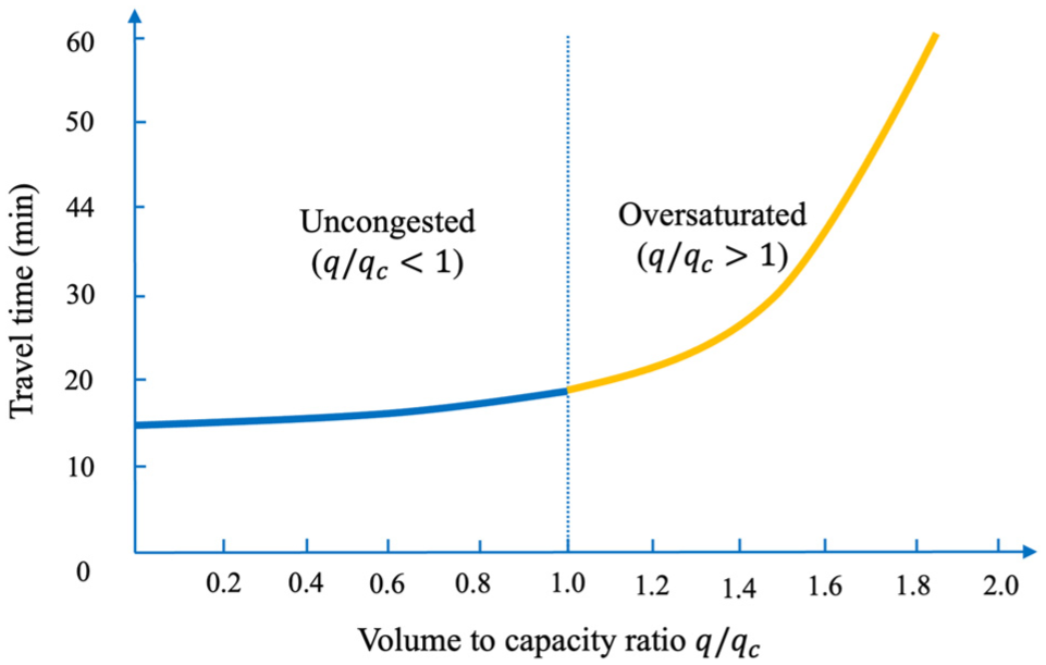
Monotonically increasing relationship between volume-to-capacity ratio and travel time.
By assuming a constant length, the estimated speed can be derived from Equations 19 and 20 as the inverse of travel time as follows:

Therefore, during the uncongested conditions, the estimated speed could be rewritten as follows:

And under the oversaturated conditions, the speed could be estimated as follows:

The relationship between speed and
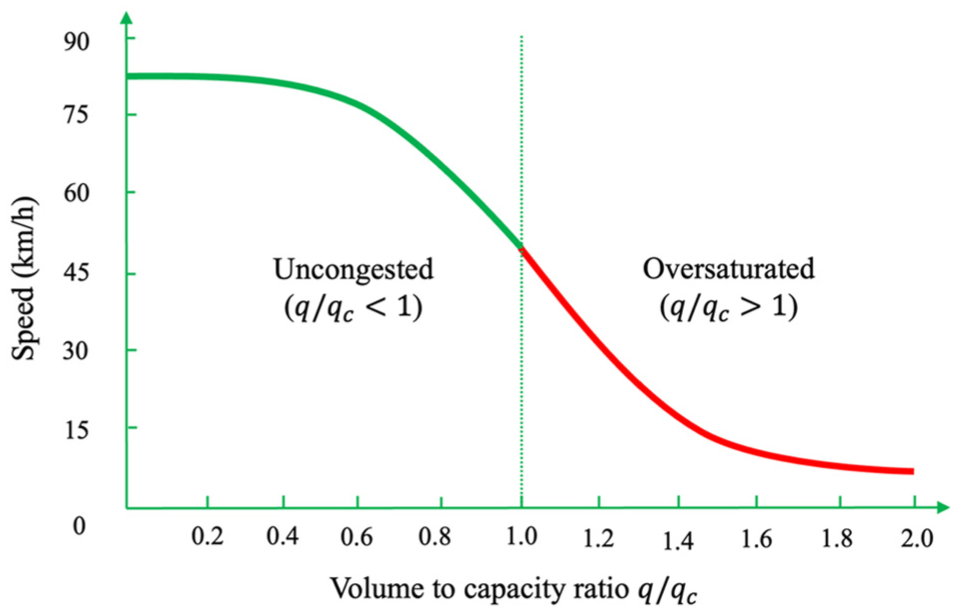
Monotonically decreasing relationship between volume-to-capacity ratio and speed.
In summary, this study derives a macroscopic traffic performance function under oversaturated conditions. When there is no traffic congestion: that is, when
Case Study
Traffic Dataset Overview
To demonstrate the effectiveness and applicability of the proposed demand estimation method under oversaturated conditions, we present two representative case studies.
Case 1: The Beijing West Third Ring corridor. This corridor extends from Wanliu Bridge in the south to Suzhou Bridge in the north, spanning a total length of 14.8 km. It comprises seven interchange bridges and 21 entrance and exit ramps, serving as a major north-south traffic corridor connecting the western urban area of Beijing. Traffic data were collected from 15 detectors along the south-to-north direction of the West Third Ring Road. Multi-day data were collected continuously over 16 days, from Monday, June 15, 2021, to Wednesday, June 30, 2021, covering both weekdays and holidays, with 24-h monitoring each day. The collected data includes traffic flow and speed, recorded at a time interval of 2 min
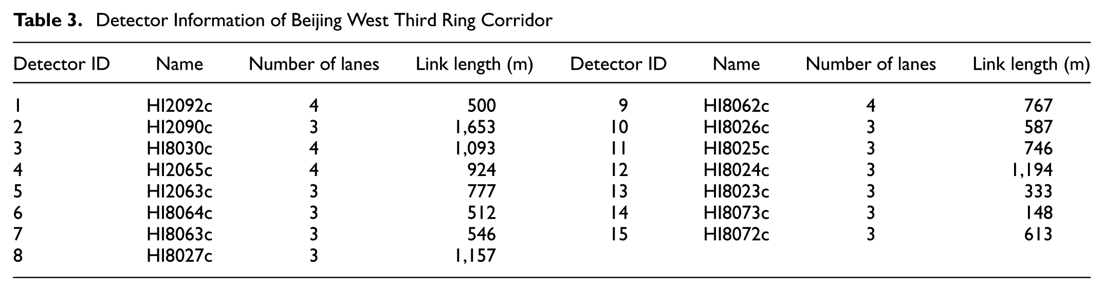
The layout of detector deployment and bottleneck locations on the Beijing West Third Ring corridor is shown in Figure 9, and detailed detector information is provided in Table 3.
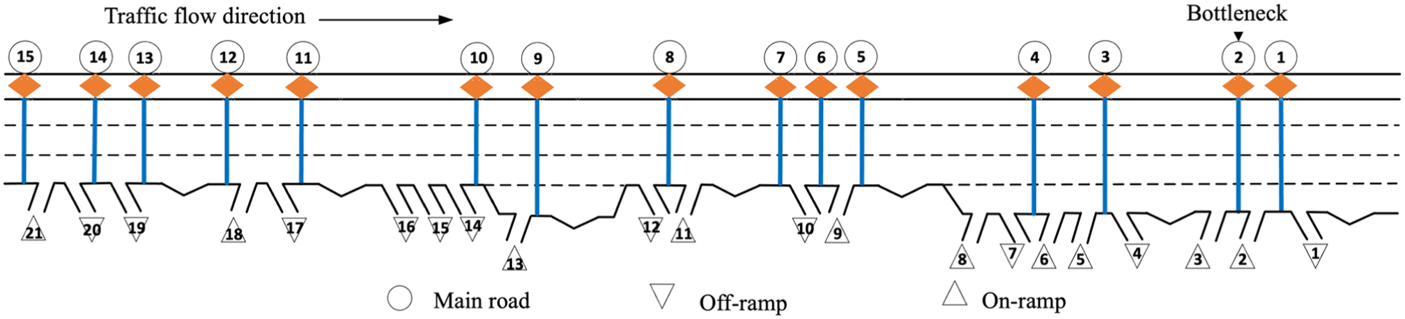
Detector deployment and bottleneck location on the Beijing West Third Ring corridor.
Detector Information of Beijing West Third Ring Corridor
Case 2: The Los Angeles (LA) I-405 corridor. This corridor is the most frequently used expressway leading to Los Angeles International Airport (LAX) and is one of the busiest roads in the United States, serving as a critical transportation artery for the West Coast region. The selected study section covers a south-to-north segment from absolute mileage 12.85 km to 23.90 km, including 22 detectors and 23 entrance and exit ramps. Traffic flow data were collected using magnetometer-based detectors. Multi-day data was collected continuously over 75 days, from Saturday, April 3, 2021, to Saturday, July 31, 2021, covering both weekdays and holidays, with 24-hour monitoring each day. The collected data include traffic flow, speed, and occupancy, recorded at a time interval of 5 min.
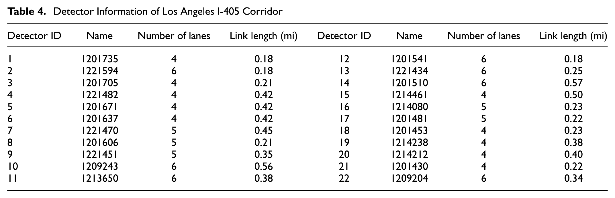
The layout of the Los Angeles I-405 corridor and detector deployment is shown in Figure 10, and detailed detector information is provided in Table 4.
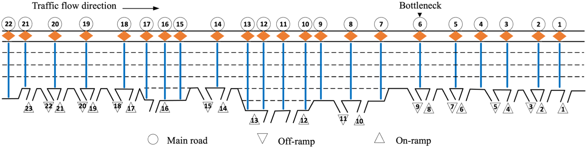
Detector deployment and bottleneck location on the Los Angeles I-405 corridor.
Detector Information of Los Angeles I-405 Corridor
Once the datasets are introduced, we proceed to calibrate FD models using observed traffic data.
Identifying Key Parameters in the Greenshields Model
To apply Equation 13 for demand estimation, we calibrate key parameters of the FD model: free-flow speed
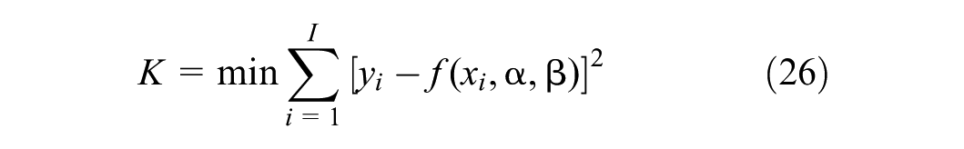
We calibrate the parameters using the least squares method (LSM), minimizing the objective function:
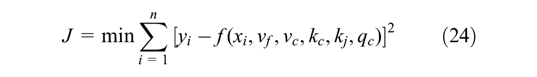
where
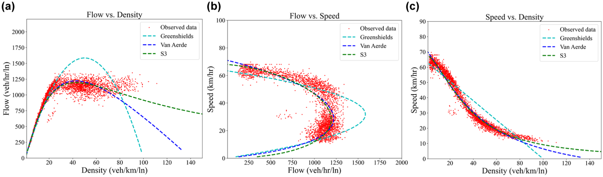
Using this method, we calibrated the key parameters of the Greenshields model, Van Aerde model ( 41 ), and S3 models ( 42 ), providing a solid foundation for subsequent traffic demand and travel time estimation. Although the Van Aerde and S3 models exhibit lower fitting errors and better overall performance, they are used primarily as benchmark models. Given that this study builds on an extension of the Greenshields model, its calibration results are adopted for all subsequent analyses.
The fitting curves for the representative cases are shown in Figures 11 and 12. The coefficient of determination (R2) reaches 0.83 for the Beijing West Third Ring dataset and 0.87 for the Los Angeles I-405 dataset using the Greenshields model, indicating a strong agreement with observed data. These results confirm that the calibrated parameters are sufficiently accurate for supporting the analyses that follow. In future work, we will consider refining alternative traffic flow models and improving demand estimation methods.
Fitting the fundamental diagram (FD) for the Beijing West Third Ring corridor: (a) flow–density relationship; (b) speed–flow relationship; (c) speed–density relationship.
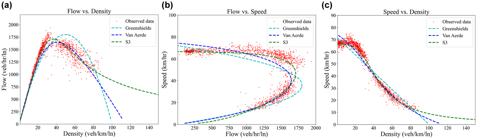
Fitting the Greenshields fundamental diagram (FD) for the Los Angeles I-405 corridor: (a) flow–density relationship; (b) speed–flow relationship; (c) speed–density relationship.
Table 5 summarizes the key calibrated parameters for the two cases across different traffic flow models. This section focuses solely on the Greenshields model. For the Beijing West Third Ring dataset, the free-flow speed is 62 km/h, with a critical speed of 31 km/h and a critical density of 45 veh/km/ln (vehicle per kilometer per lane), resulting in a capacity of 1,380 vphpl. The jam density is 100 veh/km/ln. In the Los Angeles I-405 corridor, the free-flow speed is slightly higher at 70 km/h. While the critical speed is higher at 35 km/h, the critical density remains the same at 50 veh/km/ln. The jam density is also 100 veh/km/ln, but the higher free-flow and critical speeds lead to an increased capacity of 1,750 vphpl. This comparison suggests that the Los Angeles I-405 corridor exhibits more efficient traffic flow, as indicated by its higher capacity and critical speed, potentially reflecting better road performance or differing traffic conditions.
The Calibration of Traffic Flow Key Parameters
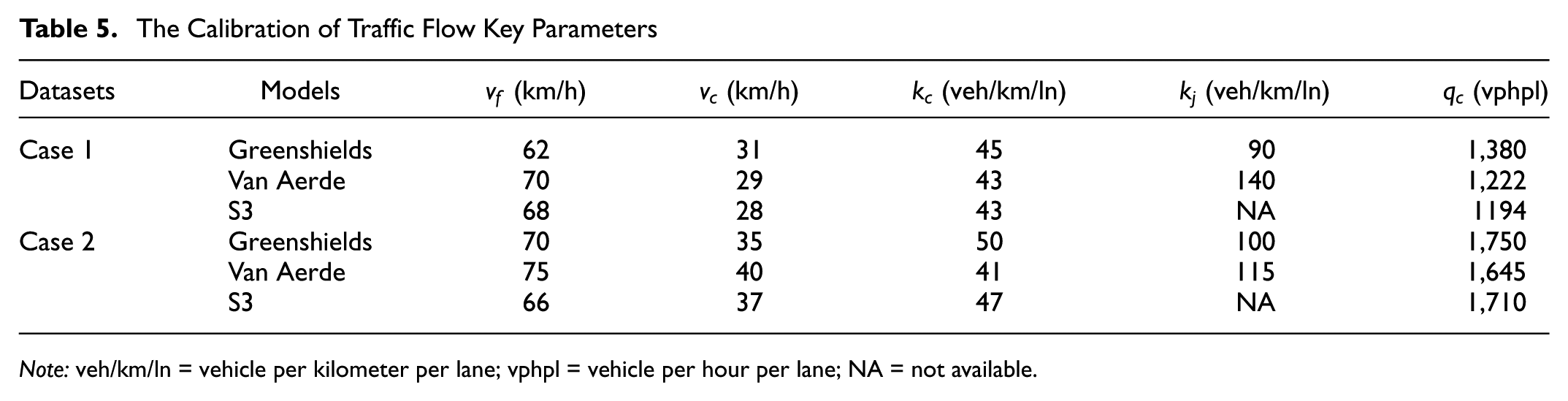
Note: veh/km/ln = vehicle per kilometer per lane; vphpl = vehicle per hour per lane; NA = not available.
Results and Discussion
Traffic Demand Estimation
Aggregate Traffic Demand Using Multi-Day Data
Based on the model calibration of traffic bottlenecks in Section 4, key parameters at the bottleneck can be obtained, as shown in Table 5. Furthermore, traffic flow can be classified into congested and non-congested states using the critical speed
Here, we introduce the average queue discharge flow during the congestion period [

The average queue discharge flow serves as a critical indicator of bottleneck outflow capacity during congestion and provides a necessary basis for inferring latent demand and accurately characterizing oversaturated traffic conditions.
The statistical analysis of multi-day data reveals the distribution of traffic demand,
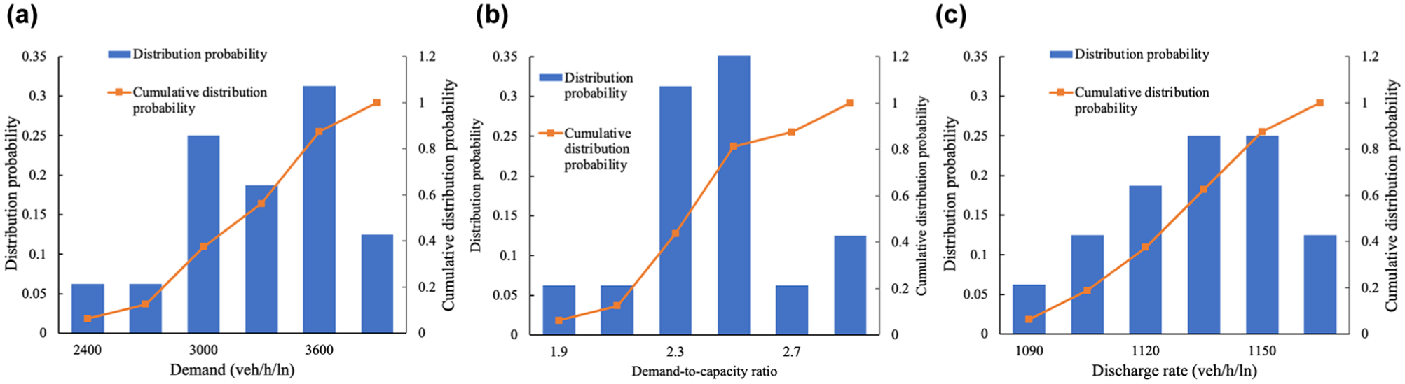
Distribution of traffic demand, demand-to-capacity ratio and discharge rate with weekday in Beijing West Third Ring corridor: (a) demand distribution, (b) demand-to-capacity ratio distribution, and (c) discharge rate distribution.
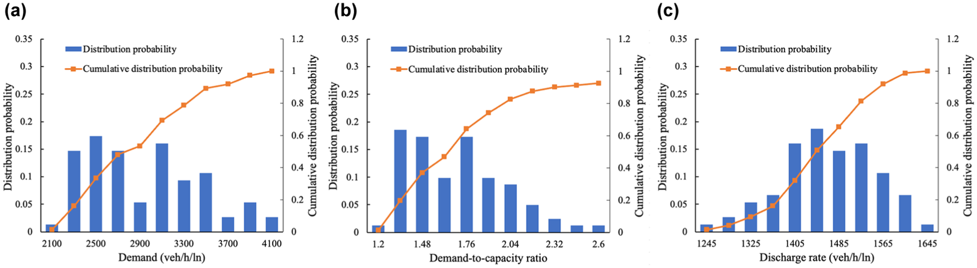
Distribution of traffic demand, demand-to-capacity ratio and discharge rate with weekday data in the Los Angeles I-405 corridor: (a) demand distribution, (b) demand-to-capacity ratio distribution, and (c) discharge rate distribution.
Overall, the average traffic demand during congestion is higher in the Beijing case than in the Los Angeles case, and the
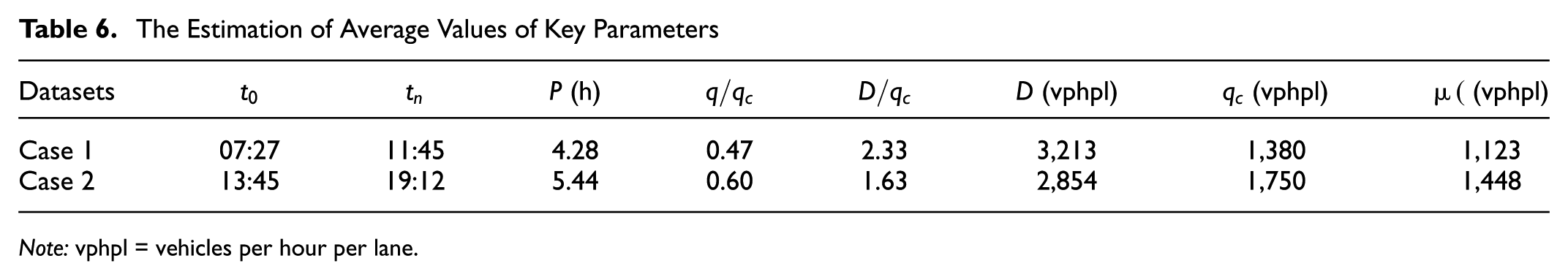
By averaging the data across multiple days, we derive the representative values of key parameters summarized in Table 6. It can be observed that the congestion duration at traffic bottlenecks in the Beijing case is 4.28 h, while in the Los Angeles case, the peak-hour congestion duration is 5.44 h. This indicates that traffic bottlenecks along the I-405 corridor in Los Angeles experience longer congestion periods than those along the West Third Ring corridor in Beijing.
The Estimation of Average Values of Key Parameters
Note: vphpl = vehicles per hour per lane.
As discussed earlier, the
Furthermore, a comparison of the dynamically estimated traffic demand, road capacity, and average queue dissipation rate during congestion is shown in Table 6. In the Beijing case, the traffic demand, road capacity, and queue dissipation rate during congestion are 3,213 vphpl, 1,380 vphpl, and 1,123 vphpl, respectively. In the Los Angeles case, these values are 2,854 vphpl, 1,750 vphpl, and 1,448 vphpl, respectively.
In both study cases, it is evident that traffic demand during congestion far exceeds road capacity, and the queue dissipation rate during congestion is lower than road capacity in both cases. Additionally, the queue dissipation rate during congestion is lower in the Beijing case than in the Los Angeles case, while the traffic demand during congestion is significantly higher in Beijing. This further confirms that congestion in the Beijing case is particularly severe.
Disaggregated Traffic Demand Estimation by Weekday Classification
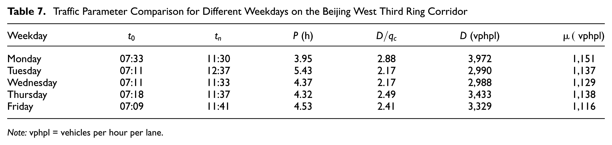
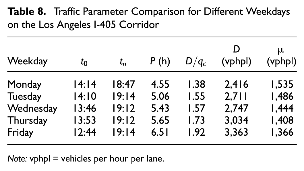
To better manage traffic demand and control traffic flow on different weekdays, we conducted an analysis based on various weekday types. The summary of the Beijing West Third Ring case is shown in Table 7, while the summary of the Los Angeles I-405 case is presented in Table 8.
Traffic Parameter Comparison for Different Weekdays on the Beijing West Third Ring Corridor
Note: vphpl = vehicles per hour per lane.
Traffic Parameter Comparison for Different Weekdays on the Los Angeles I-405 Corridor
Note: vphpl = vehicles per hour per lane.
The results indicate that in the Beijing West Third Ring case, the maximum
Travel Time and Speed Estimation
In this section, we use LSM to estimate travel time and speed, corresponding to Equations 26 and 27, respectively. The observed travel time data are fitted using Equation 19 for uncongested conditions and Equation 20 for oversaturated conditions, and the observed speed data are fitted using Equation 22 for uncongested conditions and Equation 23 for oversaturated.
Specifically, this involves minimizing the following objective functions for uncongested and oversaturated conditions:
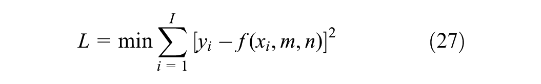
where
We used symmetric method (
11
,
20
,
21
) and quasi-density method (
13
,
35
) as the benchmark model and compared the travel time and speed estimation between the benchmark model and our proposed model. The evaluation metrics are the mean absolute percentage error (MAPE) and R2. The travel time fitting results in oversaturated conditions are shown in Figure 15. In oversaturated regions, the symmetric method yields
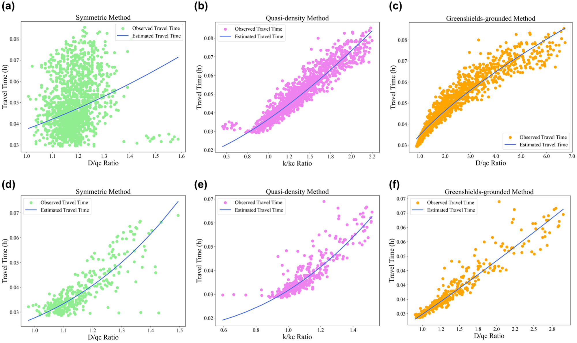
Travel time fitting results among different cases: (a) symmetric method in Beijing case; (b) quasi-density method in Beijing case; (c) proposed method in Beijing case; (d) symmetric method in the Los Angeles (LA) case; (e) quasi-density method in the LA case; (f) proposed method in the LA case.
Although all three methods use the same BPR functional form, their estimation accuracy varies owing to differences in how demand is modeled. The symmetric method applies a mirrored demand estimate; however, it is not suitable under oversaturated conditions as its range does not exceed 2. The quasi-density method uses density-based
Table 9 compares the travel time performance of the symmetric method, quasi-density method, and the proposed method in two cases using MAPE and R2 as evaluation metrics. In Case 1, the symmetric method yields a MAPE of 18.51% and an R2 of 0.21, the quasi-density method achieves a MAPE of 5.91% and an R2 of 0.94, while the proposed method slightly improves the performance with a reduced MAPE of 5.15% and an increased R2 of 0.95, which indicates enhanced prediction accuracy and better model fit. In Case 2, the advantage of the proposed method becomes more pronounced. Its MAPE significantly decreases to 3.86%, compared with 8.54% for the symmetric method and 6.56% for the quasi-density method. Its R2 also improves from 0.83 to 0.95, demonstrating superior accuracy and improved model fit in this scenario. Overall, the proposed method outperforms the benchmark models in both cases, especially in Case 2, suggesting it is more suitable for estimating and predicting traffic demand under oversaturated conditions.
Comparison of Travel Time Estimation Errors in Oversaturated Conditions
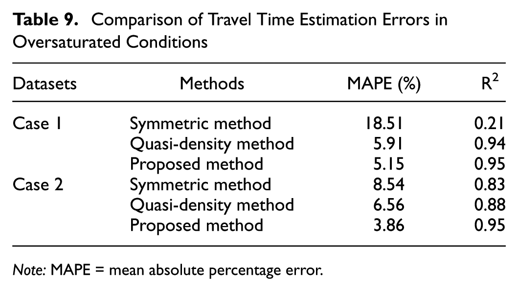
Note: MAPE = mean absolute percentage error.
Table 10 compares the speed estimation errors of the benchmark methods and the proposed method in two cases. In Case 1, the symmetric method yields a MAPE of 19.92% and an R2 of 0.13, while the quasi-density method achieves a MAPE of 6.22% and an R2 of 0.93. The proposed method further reduces the MAPE to 5.30% and improves the R2 to 0.96, indicating better estimation accuracy and model fit. In Case 2, the proposed method shows a more substantial advantage, with the MAPE dropping from 8.28% (symmetric method) to 4.05%, and the R2 increasing from 0.82 to 0.96. These results suggest that while the quasi-density and proposed methods perform similarly in Case 1, the proposed method demonstrates a clear improvement in Case 2, particularly under oversaturated conditions. The fitting results for speed are illustrated in Figure 16, which align with the patterns observed in Figure 8b under over-saturated conditions.
Comparison of Speed Estimation Errors in Oversaturated Conditions
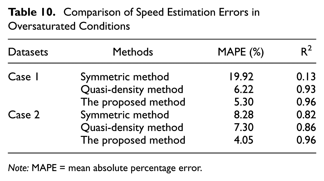
Note: MAPE = mean absolute percentage error.
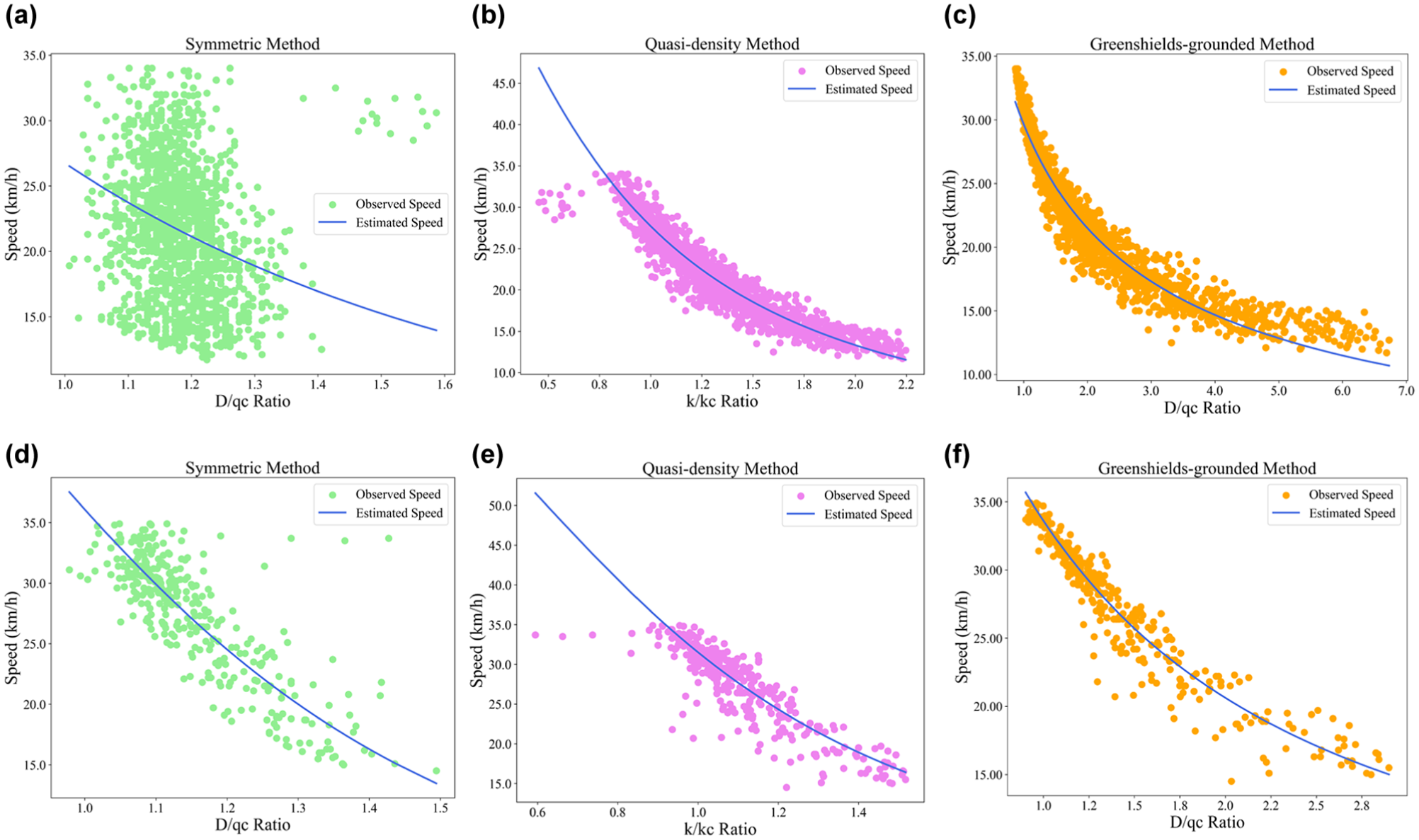
Speed fitting results among different cases: (a) symmetric method in Beijing case; (b) quasi-density method in Beijing case; (c) proposed method in Beijing case; (d) symmetric method in the Los Angeles (LA) case; (e) quasi-density method in the LA case; (f) proposed method in the LA case.
As shown in Tables 9 and 10 and Figures 15 and 16, the symmetric method fails to provide satisfactory estimation performance for both travel time and speed in the Beijing case. This is primarily owing to its inherent limitation in representing demand when the
Travel Time Index Analysis
The Travel Time Index (TTI) is an indicator used to measure the level of traffic congestion. It represents the ratio of travel time under congested conditions to travel time under free-flow conditions. TTI is commonly used to quantify the efficiency of road systems and helps transportation planners and researchers assess the severity of traffic congestion. It can be calculated as follows:

Further, we could derive the following Equation 29 for estimate TTI for uncongested conditions and Equation 30 for estimate TTI for oversaturated conditions.


In the section ‘Identifying key parameters in the Greenshields model’, by fitting the proposed model with observation data, we could derive the calibrated parameters
The Results of Calibrated Parameters and Estimated Travel Time Index (TTI)
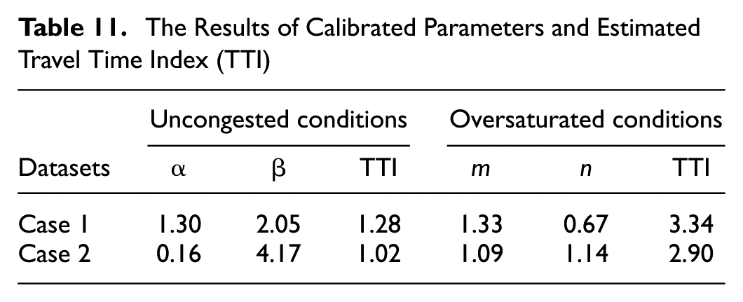
Furthermore, from the calibrated parameters, Case 1 has
This finding demonstrates that the proposed model more accurately reflects traffic conditions when congestion occurs and better captures the relationships between traffic variables in oversaturated traffic systems. The travel time index obtained using this method is more reliable and provides a more accurate estimate of traffic congestion.
Analysis of Congestion Causes and Regional Differences
The analysis of the causes of congestion on urban expressways can be summarized from two perspectives: travel demand and road supply.
From the perspective of travel demand, the fundamental reason for congestion is that traffic demand exceeds the road supply capacity. Travel demand is reflected in the origin–destination characteristics of individual trips and the traffic volumes observed at expressway entrances and exits. Additionally, a significant number of lane-changing behaviors occur near expressway ramps and weaving areas, especially during congestion periods. These lane changes increase traffic demand, as drivers attempt to avoid long queues by switching lanes. From the perspective of road supply, urban traffic planning and the structural design of expressways also contribute to congestion. Expressway congestion is associated with several factors, including insufficient road infrastructure, structural design issues, job-housing imbalance, road network density, road hierarchy, insufficient lane capacity, excessive weaving zone length, the number of entrances and exits, spacing between ramps, and the presence of dedicated bus lanes. These factors influence the capacity and smoothness of expressway traffic flow.
The analysis of urban expressway congestion can also be categorized into dynamic and static causes. Dynamic causes of congestion include the mainline traffic volume on expressways, the traffic volume at entrance and exit ramps, and the frequency of lane changes in weaving areas. Static causes of congestion include the job-housing separation ratio, road network structure such as network density, road hierarchy, and the capacity to accommodate through traffic, roadway infrastructure including the number of mainline lanes, the length of weaving zones and transition sections, the number of interchanges, and the presence of dedicated bus lanes, as well as entrance and exit ramps with reference to their number, types, and spacing.
Table 12 summarizes several factors that may influence congestion across the two case study corridors, including road supply capacity, traffic demand, dedicated bus lanes, job-housing separation, number of mainline lanes, number of entrance and exit ramp, and total corridor length. Beijing West Third Ring Road functions as a major urban arterial that links the northern and southern parts of the city. In comparison, Los Angeles I-405 freeway offers essential access to LAX and ranks among the busiest expressways on the West Coast.
Comparison of the Causes of Traffic Congestion Between Two Cases
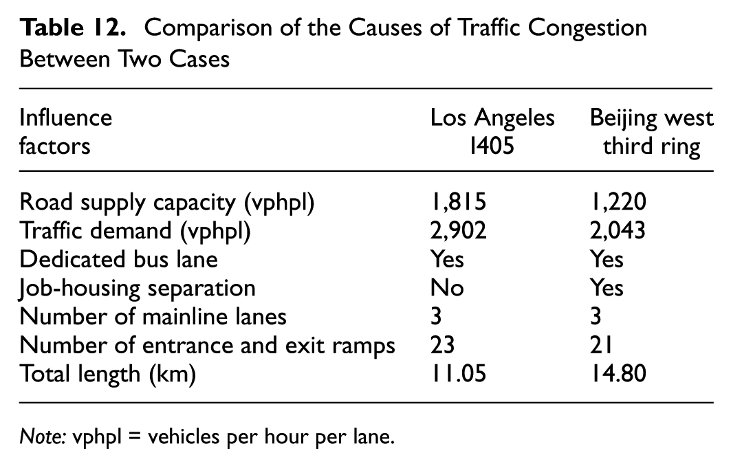
Note: vphpl = vehicles per hour per lane.
Supplementing this, Table 6 shows that traffic demand on West Third Ring corridor in Beijing is significantly higher than that on the Los Angeles I-405 corridor, while its capacity
While job-housing separation may be one contributing factor to Beijing’s higher congestion levels, this interpretation remains descriptive and should not be interpreted as causal. Other contextual factors, including land use distribution, traffic signal control, and vehicle ownership rates, may also play important roles. Our current analysis does not disentangle these variables; thus, future research could employ multivariate or causal modeling approaches to quantify their individual contributions.
In summary, the comparative case study highlights the value of the proposed demand estimation method in accurately capturing travel demand and congestion levels under oversaturated conditions. The findings also underscore the need to consider regional and structural factors when interpreting traffic performance and designing targeted mitigation strategies.
Limitations of the Greenshields-Based Framework
While the Greenshields model offers analytical tractability and has been widely applied in macroscopic traffic flow modeling, its assumption of a linear speed–density relationship does not fully capture the nonlinear characteristics of real-world traffic, particularly under oversaturated conditions. Our empirical analysis presented in Figure 11 shows that vehicle speeds often stabilize during congestion rather than continue to decline, forming a plateau-like region that deviates from the classical Greenshields curve.
This observation suggests that the model may not adequately reflect congested flow dynamics in dense urban networks. Although the proposed correction term improves demand estimation consistency under these conditions, it does not account for all sources of estimation error, such as variations in driver behavior, unexpected incidents, or network-level interdependencies. Therefore, the Greenshields model should be interpreted as a first-order approximation rather than a fully realistic representation of oversaturated traffic.
To improve applicability, future work may explore more flexible formulations of the FD, such as triangular or trapezoidal models, or integrate hybrid empirical–theoretical approaches that allow better modeling of stabilized-speed behavior and flow breakdown mechanisms.
Conclusions
This study proposes an improved traffic demand estimation method suitable for oversaturated traffic conditions by extending the Greenshields model with the introduction of real-time inflow rates as an adjustment parameter. A modified LPF incorporating the
Furthermore, a comparative analysis of the two case studies reveals that the Beijing West Third Ring Road exhibits higher traffic demand, lower road capacity, and a lower average queue discharge rate compared with the Los Angeles I-405 corridor. A macroscopic analysis indicates that job-housing separation is the primary cause of severe congestion in the Beijing West Third Ring Road corridor, whereas the Los Angeles I-405 corridor benefits from a more balanced urban structure, leading to lower congestion levels.
By optimizing existing traffic demand estimation models, this study enhances their applicability to oversaturated traffic conditions, thereby improving the accuracy of congestion forecasting and transportation planning. Future research directions include:
(1) Artificial intelligence techniques can be integrated to enhance the accuracy of real-time traffic demand estimation. This includes leveraging deep learning models such as long short-term memory (LSTM), graph neural networks (GNN), and Transformer architectures to capture complex traffic patterns, as well as applying reinforcement learning to optimize flow control strategies.
(2) Improving the continuity of segmented estimation by employing Bayesian inference or time-series smoothing algorithms to ensure consistency in flow estimation across different road segments.
(3) Expanding the study to large-scale traffic network assignment, exploring optimization approaches based on dynamic traffic assignment, constructing cross-resolution segment flow interactions, and utilizing multi-agent reinforcement learning to optimize route selection, thereby enhancing the overall network traffic distribution balance and efficiency.
Footnotes
Author Contributions
The authors confirm contribution to the paper as follows: study conception and design: Yuyan (Annie) Pan, Xianbiao Hu; data collection: Yuyan (Annie) Pan; analysis and interpretation of results: Yuyan (Annie) Pan; draft manuscript preparation: Yuyan (Annie) Pan, Xianbiao Hu, Qing Tang, Yanyan Chen, and Xuesong (Simon) Zhou. All authors reviewed the results and approved the final version of the manuscript.
Declaration of Conflicting Interests
The authors declared the following potential conflicts of interest with respect to the research, authorship, and/or publication of this article: Xianbiao Hu is a member of Transportation Research Record’s Editorial Board. All other authors declared no potential conflicts of interest with respect to the research, authorship, and/or publication of this article.
Funding
The authors received no financial support for the research, authorship, and/or publication of this article.
Data Accessibility Statement
The data used to support the findings of this study are available from the corresponding author on request.