
Abstract
Estimates of future switching times for traffic signals are mandatory information to enable Green Light Optimized Speed Advisory (GLOSA) or similar eco-drive applications. Because of the adjustment of the signalization to match current traffic situations, obtaining reliable switching time estimates for traffic-actuated signals is challenging because they are not derivable based on bare statistics. An expectation in machine learning (ML) algorithms is that they can identify and learn existing causalities and relations based on provided data. Considering this, the most recent research focusing on predicting traffic-actuated signals’ switching times utilizes predictive ML models trained with historical switching times and detector data. Nevertheless, these algorithms probably cannot comprehensively capture each intrinsic relation and boundary condition existing in signal programs. Therefore, a general exclusion of implausible predictions, which, for example, violate permitted green windows or durations, should not be taken for granted. Considering this, this paper presents a methodology for testing the plausibility of predictive ML model outputs, enabling further evaluations of the reliability of applied predictive models. The methodology further incorporates procedures for preventing, identifying, and adjusting implausible switching time predictions, aiming to enhance the reliability of switching time predictions for traffic-actuated signals. The performance of the developed procedures is evaluated using prediction experiments conducted with historical data from multiple real-world traffic-actuated signal systems. The results indicate that the developed procedures can contribute to enhanced forecast accuracy. The magnitude of the achievable accuracy gains, thereby, depends on the existing generalization degree of the applied predictive models.
Keywords
Green Light Optimized Speed Advisory (GLOSA) and similar Cooperative Intelligent Transport Systems (C-ITS) eco-drive applications provide drivers (human or (semi-)autonomous) with strategies, for example, speed recommendations, to avoid unnecessary braking, stopping, and acceleration maneuvers in front of traffic signals. As shown (e.g., in [1–9]), their application promises reduced fuel or (electric-)energy consumption and decreasing quantities of emitted pollutants and greenhouse gases. Various approaches cover the development and evaluation of GLOSA and eco-drive algorithms. To reduce waiting times and fuel consumption, for example, (10–13) propose algorithms incorporating upcoming traffic signal information within the vehicle’s adaptive cruise control system.
Unfortunately, in the scope of GLOSA/eco-drive related studies, traffic signals are often assumed to be pretimed, or the future switching times, which are a mandatory input for optimizing the driving strategies, are assumed to be known. Only a few studies consider traffic-actuated signals, which are, however, most prevalent in urban areas where GLOSA is expected to be most effective ( 14 ). Because the current traffic in the intersection area influences the control decisions of traffic-actuated signal control, the traffic signal controllers cannot forecast their behavior. Therefore, to provide switching time information for traffic-actuated signals, these switching times must be explicitly predicted. The accurate prediction of switching times—and the general lack of these predictions—currently pose an unresolved challenge, despite their role in enabling the practical application of GLOSA and similar eco-drive systems for actuated signals. Consequently, the benefits of GLOSA (for actuated signals) cannot be utilized until a way is found to provide accurate estimates of phase durations and switching times ( 14 , 15 ).
Some approaches, for example, (16–19), which focus on or incorporate the prediction of traffic-actuated signals switching times, incorporate historical switching time data but do not consider detector parameters. However, bare switching time statistics are insufficient to provide accurate estimates, especially when certain phases must be requested to be switched (which is generally indicated with the help of detectors); a similar situation applies when green times can vary sufficiently in relation to length and position in the cycles. According to the findings of Stevanovic et al. ( 15 ) and Krumnow et al. ( 20 ), this is even the case if the incorporated switching time statistics originate from periods under the same traffic conditions. Consequently, most of the recent research on switching time forecasts (STF) of traffic-actuated signals aims to predict future signalization by utilizing historical data from traffic signals, including detector data, and applying machine learning (ML) algorithms for training predictive models. These models are explicitly trained to directly predict certain switching events based on (current) input data. While some works, for example, (21–23), compare the performance of different ML algorithms to predict the switching times of traffic-actuated signals, others focus on evaluating the performance of specific algorithms. In Weisheit and Hoyer ( 24 ), the application of support vector machines is proposed. Eteifa et al. ( 25 ) describe a long short-term memory neural network-based approach. A graph-based Bayesian approach, suited to predict switching times of traffic-actuated signals, operated with a stage-oriented signal control, is presented by Bodenheimer et al. ( 26 ). In Heckmann et al. ( 27 ), we presented a similar approach. However, the scope of stage-oriented approaches is limited because not every intersection’s signalization is controlled in a stage-oriented manner. In Heckmann et al. ( 28 ), we presented an approach to predict traffic-actuated signals by predicting future sequences of general states of signalization involving the application of Extreme Gradient Boosting (XGBoost). This approach is tuned to provide predictions of the state and switching times of each motorized traffic-related signal (MT signals) of the target intersection for a defined minimal prediction horizon of 30 s. Therefore, this approach overcomes the flaw of systematically inconstant-sized covered prediction horizons, which is present in other approaches.
A key expectation in ML algorithms is that they can identify existing patterns, causalities, and relationships based on the provided training data. Theoretically, this provides the advantage of allowing the rolling out of an ML-based STF approach to predict the switching times of various intersections without requiring excessive effort by a human engineer (or programmer) to manually implement or consider each relationship between multiple features and the target values. The contribution of expert knowledge (e.g., in relation to how traffic signal systems operate) should, nevertheless, be considered beneficial for providing reliable and well-performing predictive models. On the one hand, by selecting and engineering valuable features and on the other hand, by tuning the hyperparameters used to train those models. These aspects have received a certain amount of consideration in the scope of previous research work. However, it is likely that, even when a carefully chosen selection of features that contain or allow it to derive any control-relevant information is provided, applied machine algorithms cannot fully capture each important intrinsic relationship and boundary condition. Therefore, without further effort, it cannot be taken for granted that the output of implausible switching time predictions is excluded with certainty. In this context and in the further scope of this paper, implausible predictions are considered as outputs that violate constraints of the signal control logic, for example, predictions that infringe on the minimum or maximum green durations or permitted green windows.
In previous research, the performance of applied predictive approaches and predictive models is generally measured by comparing predicted values with the ground truth to calculate specific evaluation scores, for example, mean absolute error (MAE) values. However, testing the plausibility of made predictions could enable a more in-depth and targeted evaluation of the performance and reliability of the applied predictive models. In particular, it might contribute to uncovering generalization deficits. Furthermore, plausibility tests can be implemented at an earlier stage, directly in the switching time prediction procedure. Therefore, implausible predictions can be identified and classified as unreliable ad hoc. Moreover, identifying implausibility at this stage allows us to perform immediate adjustments of the prediction output.
In this context, this paper investigates how this potential can be exploited and evaluates whether the additional effort is worthwhile. To the best of our knowledge, an approach that combines an ML-based approach with a plausibility check to identify and adjust implausible predictions has not been covered in the field of STF. This paper builds on the framework and findings of our previous research ( 28 ). To develop and implement procedures for identifying and adjusting implausible predictions, knowledge about the operation of traffic signal systems, as well as historical switching time and detector data, is utilized.
Methodology
To provide answers to the previously formulated research questions, prediction experiments with historical switching time and detector data of a real-world traffic-actuated signalized intersection are conducted and evaluated.
For conducting those switching time predictions, the existing framework of the STF approach presented in Heckmann et al. ( 28 ) was utilized, systematically adapted, and extended. In total, a four-step research methodology was undertaken.
In the first step, the historical data from a chosen traffic-actuated signal system was preprocessed and prepared for the application of XGBoost. The second step involved developing procedures for preventing, identifying, and adjusting implausible predictions, which were then implemented in the existing framework. The third step was testing these procedures with prediction experiments and evaluating whether they could provide performance benefits to predict the switching times of the chosen traffic-actuated signal system. In the last step, the developed procedures were applied to the historical data of additional intersections with traffic-actuated signal systems to evaluate the generalizability of the findings.
Prediction Concept
At signalized intersections, each connected signal’s state and switching times are determined by the signal control unit, which operates based on defined rules, always ensuring that the overall intersection’s signalization is in a state that ensures traffic safety. Therefore, the current overall state of an intersection’s signalization can be considered as the combination of the current state of each intersection’s signal. Considering this, the main idea of the applied STF approach in this paper is to determine the switching times of motorized traffic-related signals (MT signals) of the targeted intersection, based on predicted sequences of the overall signalization states of motorized traffic (MTSSt).
The approach’s key methodology is exemplified with a simplified signal timing plan, as shown in Figure 1. The target features, for applying predictive ML models, are the future switched MTSSt (
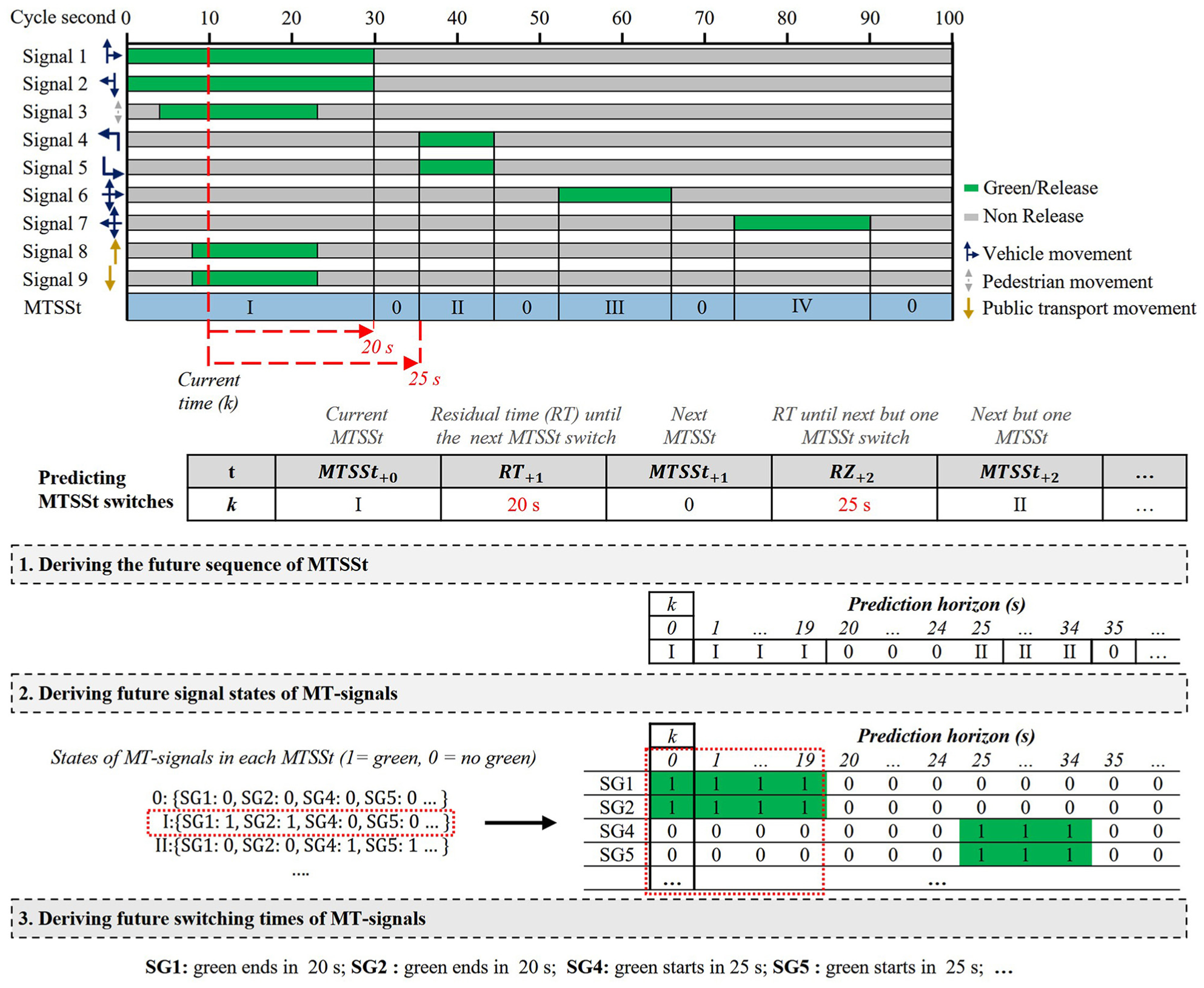
Methodology for deriving future switching times of MT-related signals by previously predicting switches of MTSSts.
A determination of the switching times of pedestrians and public transport vehicles was omitted because those user groups are not the potential primary users of the GLOSA or eco-drive applications. In addition, this simplification is beneficial because the number of switched distinct MTSSts is significantly lower than the number of unique overall signal state combinations if the states of each road user’s signals were considered. Furthermore, the methodology applies to distinct types of applied phasing schemes, whether a National Electrical Manufacturers (NEMA) scheme, phasing schemes of the German Guidelines for Traffic Signals (RiLSA [ 29 ]) (stage- or signal group (SG) oriented signal control), or comparable schemes are applied. In cases where, for example, all MT-related signal heads involved in a certain phase always show green at the same time, the number of unique MTSSts would correspond to the number of unique simultaneity switchable combinations of phases and an offset state in which each MT signal’s state is red.
For predicting the targets relating to future MTSSt switches based on the results of our previous studies ( 22 , 27 , 28 ), the Python implementation of the ML algorithm XGBoost ( 30 ) is applied. XGBoost is a gradient boosting framework that uses an ensemble of decision trees to make predictions. Therefore, each tree is trained to correct the errors of the previous tree. To prevent overfitting, the algorithm includes regularization.
Data Description and Preparation
The historical data of Intersection 002 Katzensprung (Figure 2), selected for the investigations of this paper, was provided to us by the German city of Kassel’s local urban traffic and roads authority. A coordinated traffic-actuated signal control with a cycle time of 100 s was applied to signal the traffic streams at the four-way intersection. Nine of the 37 signal groups engage in signaling MT-related movements. For adjusting the signalization to the current traffic, information gathered by 37 detectors was used (see Figure 2).
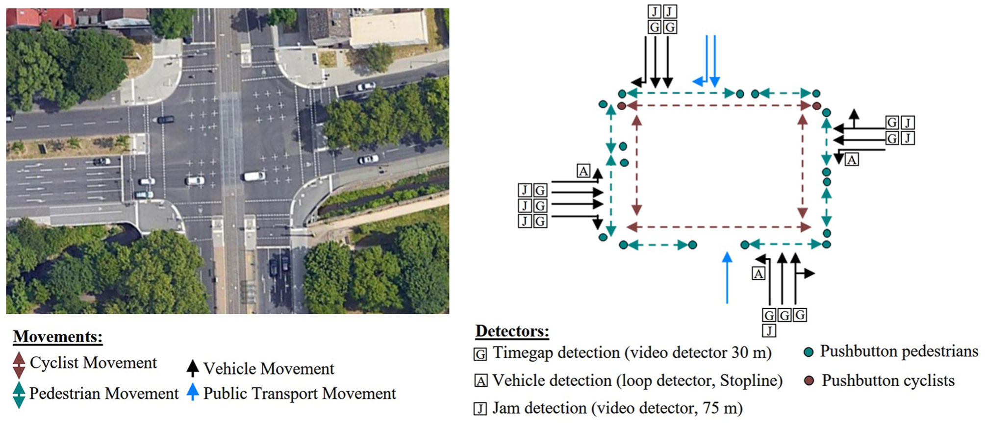
Signalized movements, lanes, and detectors at Intersection 002.
The signal control is operated stage-oriented. According to the RiLSA, a stage is “a part of a signal program during which a given signalization status remains unchanged” ( 29 ). The period of a stage reaches from the green start (GS) of the last released stream until the next green end (GE) of any released stream. Therefore, the green times of traffic streams that have the right of way during the same stage must not start simultaneously. Because of differing distances to conflict zones and for optimizing the efficiency of the intersection’s signalization, offsets between the GSs of traffic streams, released in the same stage, are often present. Furthermore, as exemplified in the stage flow shard of Intersection 002, several non-conflicting traffic streams can have the right of way during the period of a stage. Transition (periods) are switched between stages and contain individual, generally predefined sequences of signaling states to ensure that conflict zones are cleared before conflicting streams are released. The 17 defined stages are divided into eight logic blocks, which are passed through cyclically, where certain blocks contain one stage, and others contain up to four distinct stages (Figure 3). Not requested blocks are skipped, and the switched stage in blocks that contain multiple stages is chosen based on the current traffic situation. Because of the implemented coordination, Stages 1 and 7 are switched in every cycle, and others, which contain, for example, public transport or pedestrian releases, are only switched if requested. However, the coordination can be abandoned in favor of public transport releases.
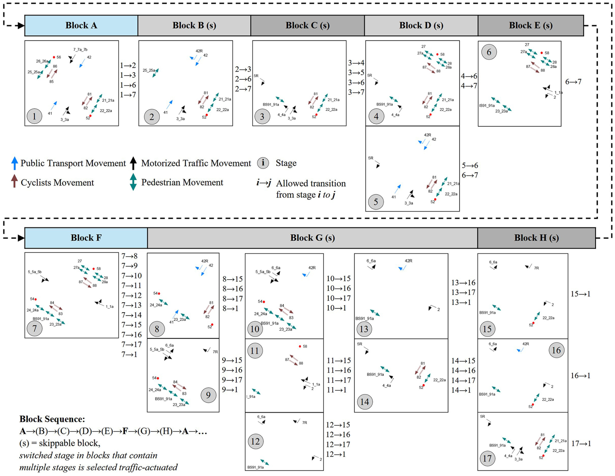
Stage flow chart of Intersection 002.
Furthermore, as shown in Figure 3, stages that contain (almost) identical released movements are held in multiple logic blocks. This enables the catch-up of green times for traffic streams that were not previously requested or were skipped because of the switching of a prioritized stage. In addition, because of a traffic-actuated control operation, referred to as transition manipulation, if certain conditions are satisfied, a running transition can be aborted in favor of a transition to another stage before the overall state of the stage is reached. As a result, deviations from the predefined characteristics of the signal state pattern of transition periods described in the RiLSA ( 29 ) are possible at the given intersection. Four different traffic-actuated signal programs (SP) tuned for specific traffic demand scenarios and traffic volumes are applied, whereby on weekends and public holidays, the operation of SP3 is omitted.
SP1: morning (peak) hours (5:30–8:30 a.m.).
SP2: daytime periods outside peak hours (8:30 a.m.–2:30 p.m. and 6:30–9:00 p.m.).
SP3: afternoon (peak) hours (2:30–6:30 p.m.).
SP4: late evening and night hours (9:00 p.m.–5:30 a.m.).
Raw Data Preparation
The provided raw data of Intersection 002 consists of daily log files, which contain cycle seconds and timestamps of signal state and detector state changes, as well as received announcement messages from public transport vehicles.
Because the data source originates from infrastructure-side logging, it does not include vehicle trajectory or driver-specific information. The same applies to environmental influences, such as weather and visibility conditions, which were not recorded, because the signal control logic at the intersection does not incorporate this information. Control decisions are primarily influenced by detector actuations (made by vehicles and pedestrians) and consider public transport priority. As a result, identical temporal constellations of detected actuations and user requests consistently lead to the same control decisions, regardless of the external conditions such as weather or visibility. Therefore, a combination of the given data source with weather or visibility-related data from external sources was omitted.
A Python script was applied to extract all relevant data of the signals related to the visualized movements and the detectors shown in Figure 2. Negotiable information in the context of STF, like the data of signal heads that only display hazard warnings, is removed. To obtain a data structure that contains the respective status of signal heads and detectors for each second, gaps between logged state changes of signal heads and detectors are filled. Periods for which no data is available for certain detectors and signal heads are cleansed. Signal states were unified and only differed between green ( = 1) and not green ( = 0). The key feature relating to the switched MTSSt is derived by assigning a unique identifier (integer number) for each unique combination of MT-related signal states that occur. A detailed description of this procedure can be found in Heckmann et al. (
28
). The target features: the future switched MTSSt (
Considering the given time series forecast task, adding information referring to previous switching and detector actuation events appeared mandatory, because XGBoost does not incorporate a built-in lookback period. Therefore, features related to the time since (TS) the last state change of signals, detectors, MTSSt, and public transportation (PT) requests were added. Consequently, features relating to previously switched MTSSts are also added. The selected extracted targets and features are summarized in Table 1. This selection also provides information like minimum and maximum green times, even if these are not provided as explicit features. For example, the highest occurring
Selection of Extracted Targets and Features
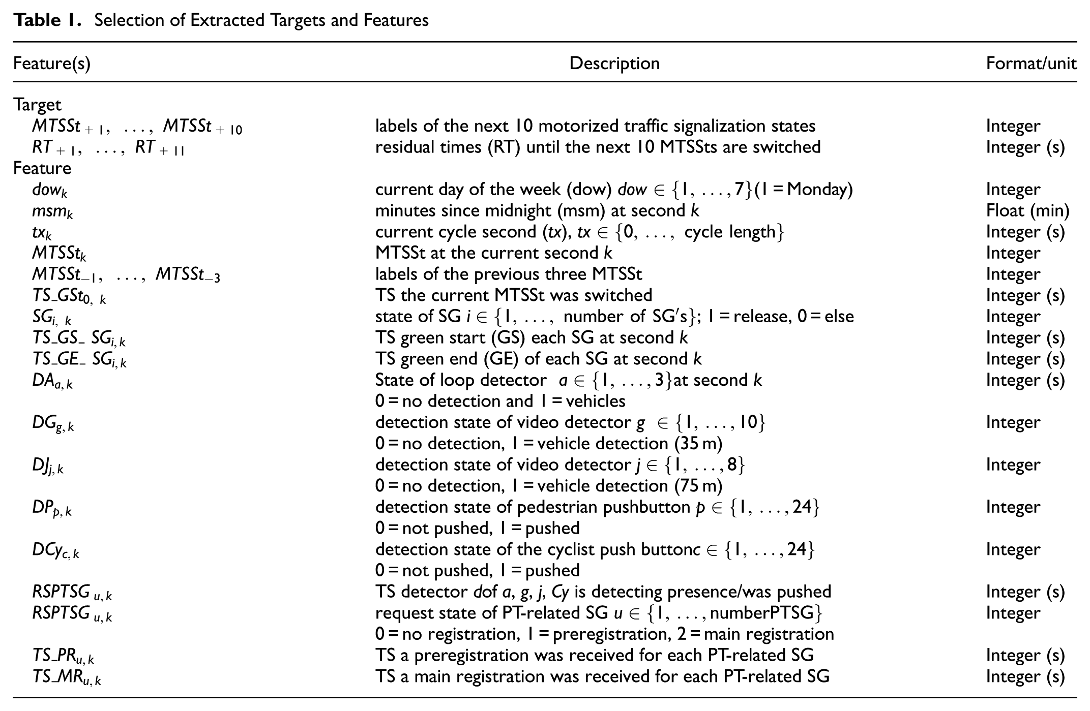
However, providing this information as explicit features or tracking if the minimum green duration of a signal is reached has not yet been shown to be beneficial. This may be because of the applied ML algorithm or the selected intersections under research. Therefore, the usefulness of providing these features should be reviewed in each application case.
Identification and Adjustment of Implausible Predictions
In the SP, boundary conditions and causalities are set (even) for traffic-actuated controlled signals.
These are, for example, regulations in relation to allowed green durations and, especially when cycle times are defined, green permission windows related to the elapsed time in the cycle. Furthermore, the spaces of allowed signal state combinations (overall states) and phasing sequences are limited to provide traffic safety or because of performance reasons. These boundaries and causalities also apply when the signalization is considered at the layer of MTSSts. As such, the space of switched MTTSts and permitted state succession sequences is also limited. Certain MTSSts only have one permitted successor; others can have multiple ones. The duration for which MTSSts are switched also relies on their position within the MTSSt sequence and the elapsed time in the cycle, but it can also be influenced by traffic.
As a result, the targets of successive MTSSt switches are related to the preceding ones. Based on a suitable selection of features extracted from current and past data, one could expect that these boundary conditions and causalities are learnable by the chosen ML algorithm. To support this, as in the chosen feature selection (Table 1), features relating to previous MTSSt switches can be incorporated. Furthermore, as in Heckmann et al. ( 28 ), a cascading prediction procedure can be applied, where previously made predictions are used as additional features for predicting switches further in the future.
However, if boundary conditions and causalities are known or can be identified, they can be used to evaluate the plausibility of made switching time predictions. Furthermore, they can be considered directly in the prediction procedure to spare unnecessary predictions. To exemplify: if a certain MTSSt only has one permitted successor state, this subsequent state must not be predicted. The causalities relating to permitted state changes can also exist within certain MTSSt sequences. Similarly, RT predictions can be spared if certain MTSSt:
are always switched for a fixed duration or,
are switched for a fixed duration within a particular state sequence.
In addition to saving effort/time by sparing unnecessary predictions, making incorrect predictions in cases where a model has not learned those causalities can be avoided. Moreover, all permitted state changes and permission periods for MTSSt related to cycle seconds can be involved. If a plausibility check reveals that a predicted state cannot follow its predecessor, the predictions can be adjusted to match the boundary. Therefore, the proportion of wrong state predictions could be reduced. Similar adjustments can be made for implausible RT values. In addition, the determined signalization and switching times of the MT signals can be checked for plausibility. This enables adjustments of identified implausible switching times as well. Nevertheless, the existing boundaries must be identified first to enable plausibility testing and subsequent adjustments. Because we were not provided with the intersection’s explicit controller logic, the historical data provided was utilized. For this, a Python script that analyses the MTTSt state sequences occurring in the data was developed and applied. This script identifies:
permissible MTSSt sequences;
permission periods of all MTSSt related to cycle seconds;
the minimum and maximum switching duration of each MTSSt.
barley and within certain sequences, and store them as key–value pairs in a Python dictionary. This is achieved by analyzing the MTSSt sequences and their durations that occur in the preprocessed historical switching time data. An appropriately large number of historical data points analyzed ensures that all switchable sequences and state durations (variations) are covered. Because of the operation mode of the script relying only on historical switching time data, they are not limited to the traffic signal system under investigation; they can also be applied to the data of traffic signal systems of other intersections.
A similar script is crafted to obtain the minimal and maximum switching durations and cycle time-related permissible green windows of each MT signal. In the following sections, these dictionaries are related to MTSSt-constrains-dict and MT-Signal-constrains-dict.
Procedure for Adjusting Implausible Predicted MTS States and Residual Time Values
Certain ML methods, like XGBoost, offer an alternative where predictive models can output a vector for all values for which they were trained. This option is often referred to as predict proba(bility). The output vector contains a confidence probability for each possible output value (predictions). Therefore, the value with the highest confidence corresponds to the value that would be the output if a default prediction is performed.
Considered in relation to an adjustment of implausible predictions, applying the predict proba method of XGBoost instead of default predictions appeared exploitable for this task. The output of confidence vectors allows the application of an iterative procedure aiming to identify the most probable value, which fulfills the set criteria of the applied plausibility test. In this iterative procedure, the output value with the highest confidence can first be checked to determine whether it is plausible. If this is not the case, the next probable value can be checked. This process can be repeated until a value that fulfills the set criteria is found. By applying such a procedure, the trained ML model and its learned relationships can still be exploited. Outside of cases where the likelihood of a switching event can be classified as certain, this procedure should be considered superior compared with picking or guessing fitting values based on bare statistics.
To identify and adjust implausible prediction outputs, we implemented a prediction framework that involves two of the described iterative procedures. One is for checking predicted MTSSt values, and another is for predicted RT values. The concept of the overall framework is shown in Figure 4. Building on an alternating prediction of RTs and future switched MTSSts, the next 10 MTSSt switches, oriented from a current second k, are covered.
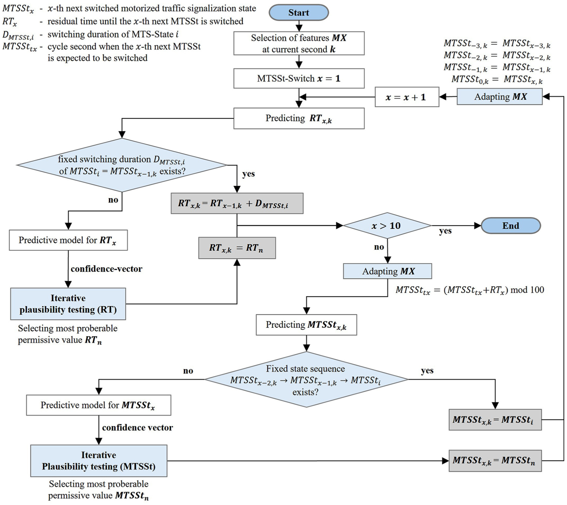
Overall framework for preventing, identifying, and adjusting implausible MTSSt and RT values.
Because
Initially, based on the MTSSt-constrains-dict, if the current switched MTSSt features a fixed duration is checked. If this is the case, none of the prediction models are utilized. Instead, the corresponding target’s value is determined based on the already elapsed switching duration of the current state and the known fixed switching duration of this MTSSt. Suppose no certain outcome, in means of a fixed duration, is derivable. In that case, the iterative plausibility check and adjustment procedure for RT predictions is triggered, which is described in detail in the following sections.
In succession of the prediction of
During the alternating prediction procedure, the feature selection is constantly adapted based on the predictions made to provide the predictive models with recent information, as described at the beginning of this subsection.
The methodologies of the procedures for identifying the most probable permissive RT and MTSSt values, which are triggered if no certain RT or MTSSt value can be determined, are shown in Figure 5. As input for both iterative procedures, the information noted in the MTSSt-constrains-dict and a confidence vector given by applying the trained predictive models are utilized. The values in the confidence vector are sorted based on the given probabilities. Then, the possible target values are evaluated for plausibility, beginning with the value with the highest confidence (
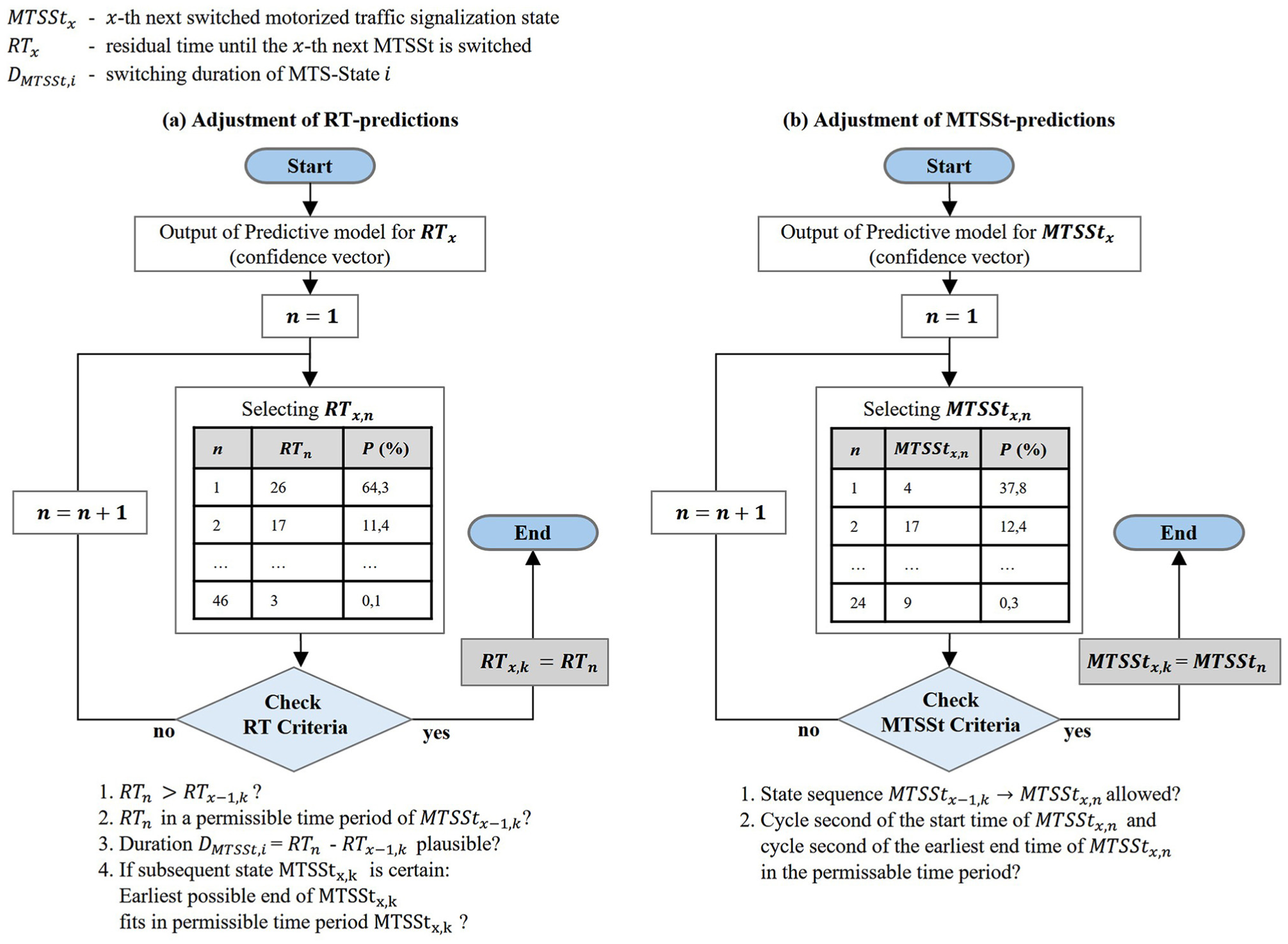
Methodologies for identifying the most probable plausible RT: (a) and MTSSt (b) values.
For RT predictions (see Figure 5a), the conditions that must be satisfied for considering an RT value as plausible are as follows. The potential RT- value until the
For the MTSSt predictions, the iterative procedure covers two conditions that must be satisfied to consider a potential next switched MTSSt as a plausible prediction for the
To prevent a no-prediction output from being made if no value is found that passes all criteria, two fallback layers are considered. For simplicity, these are omitted in Figure 5. As a first fallback, the output value with the highest initial confidence, which satisfies most of the criteria, is chosen. If such a value does not exist, the most confident value based on the confidence vector is chosen.
In relation to the mentioned fallback layers, these layers may not be triggered within the first MTSSt and RT predictions; they become more relevant with an increasing temporal horizon, where uncertainties for checking for permissible time periods may evolve.
Procedure for Adjusting Implausible Determined MT Signal’s State Sequences
A further procedure was developed to check the MT-Signal-state sequences derived from the MTSSt switch predictions for implausible outputs (Figure 6). The procedure can be used independently or in succession to the procedure shown in Figure 4. In a first step, based on the MT-Signal-constrains-dict, green states for time periods outside the permissive periods are removed. Then, the predicted remaining duration of currently running green periods is checked for plausibility. Because these periods have already started, the predicted duration can be checked to see if it is within the scope of the minimum and maximum allowed green durations. This allows shortening of too long periods and lengthening of too short ones with high confidence (see Figure 6). In the last step, existing leftover, too short periods located in the derived sequences are cleansed. For each SG, an individual threshold value that depends on the minimum allowed green duration is chosen.
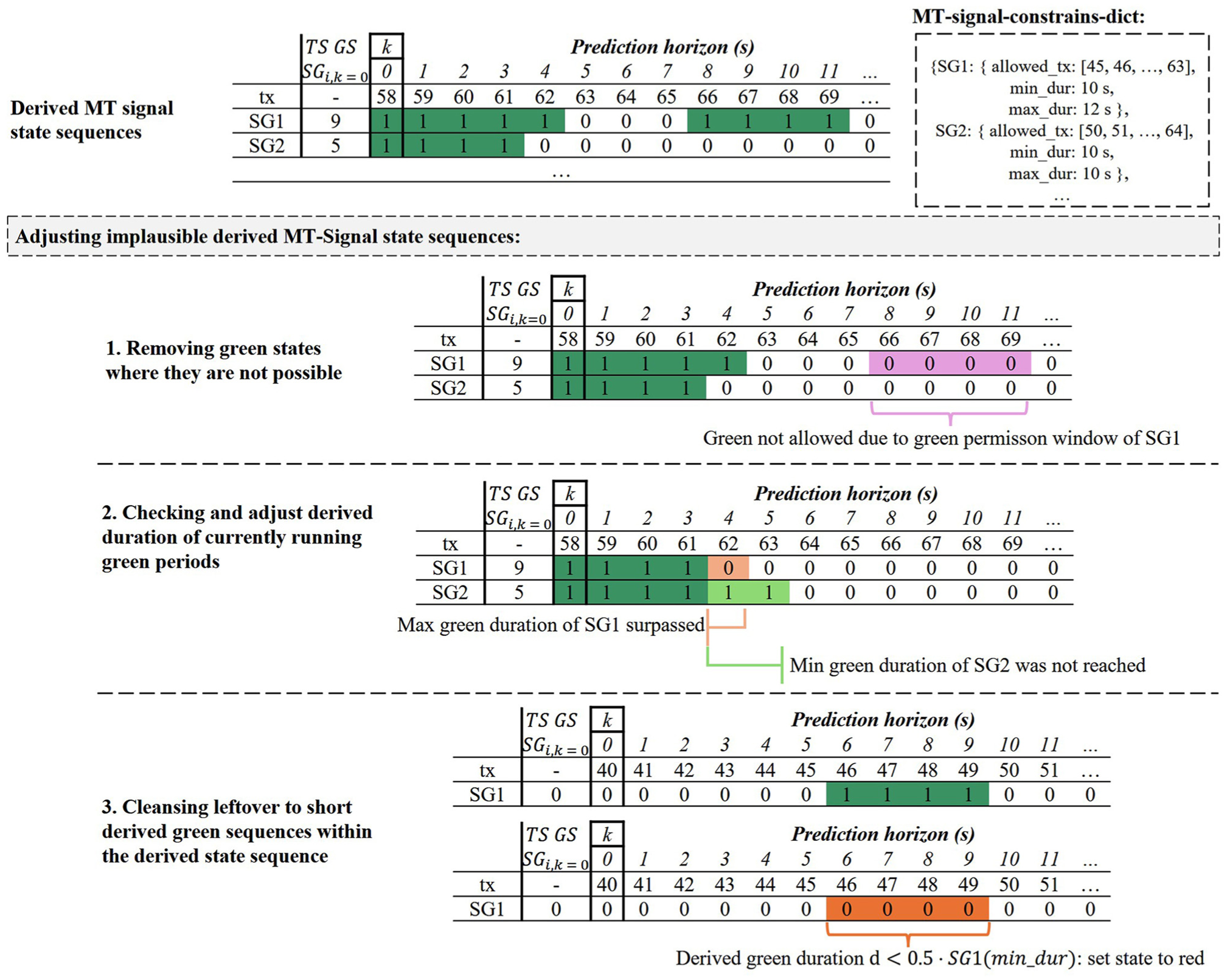
Methodology for plausibility testing and adjusting derived MT-signal state sequences.
Prediction Experiments
To test whether the application of the previously described procedures that consider given boundary conditions and restrictions for preventing, identifying, and adjusting implausible switching time predictions is beneficial, prediction experiments are conducted. In the scope of those experiments, besides the baseline case (0) in which neither of the procedures is applied, each application combination is considered.
Adjusting MTSSt-switch-predictions (A) (Figure 4)
Adjusting derived MT-signal state sequences (B) (Figure 6)
Applying both procedures (A + B)
To consider differing traffic loads and demand scenarios, ranging from average to peak traffic volumes, data models based on raw data logged during the active time of SP2 and SP3 between February and April 2023 are selected.
For each SP, the selected data models are split into different training and test data sets. For SP2, all samples of the previous month, except the last 200,000 instances, are selected as training data, and the first 400,000 samples of the following month are selected as test data. The spared last 200,000 samples of the previous month are selected as validation data for the training procedure. For SP3, the same splitting procedure is applied; however, because of SP3’s lower monthly runtime, a reduced sample sizes of 150,000 for the test data and 50,000 samples for the validation data are selected. The comparatively high numbers of continuous test samples are selected to cover the scope of different daily and weekly demand scenarios, and because of the condition that continuous predictions for the future would be required in a real-time application.
Each training data set is used to train predictive models for the 21 defined target features described in the first subsection. Adaptations of the feature selection related to the previously switched MTSSt, as shown in Figure 4, are made in the training procedure. For these training tasks, the real target values of previous switches are used. The applied sets of hyperparameters were optimized and chosen based on a grid search conducted with data models consisting of historical data from January 2023.
The trained models are applied to the test data sets for each of the four application cases. For the predictions for the baseline case, the same alternating prediction order, as shown in Figure 4, is used, but neither adjustment nor setting procedures for safe outcomes are applied. Therefore, the output of the predictive models remains unchanged.
Results and Discussion
To compare the performance of the application cases and to evaluate the reliability of the made switching time predictions, an evaluation horizon of 30 s, equal to the minimal provided horizon to be covered by predictions, is chosen, and the evaluation metrics described as follows are used.
The accuracy (ACC, Equation 1) is considered as the share of signalization sequences of MT signals, covering their signal states for the next 30 s, which are predicted accurately to the second, without any deviation. In Equation 1, sequences that entirely match the ground truth are denoted as true positives (TP). Deviating sequences are denoted as false positives (FP). Because not every sequence must cover a signal change (SC), additional individual accuracy scores are calculated for sequences that contain at least one signal change (switch sequences) and sequences that do not contain any signal change (non-switch sequences).
In a GLOSA application case, the correct SC from red to green and vice versa must be predicted with only minor deviations. Minor deviations might be tolerable if there is a large temporal distance from the switching event. Therefore, the following additional measures are used for evaluation.
The positive predictive values (PPV in Equation 2) provide the ratio of predicted SCs that match the ground truth. In contrast, the sensitivity (true positive rate [TPR] Equation 3) provides the ratio of correctly predicted SCs to all actual signal changes of the ground truth. In Equations 2 and 3, correctly predicted SCs are denoted as TP, and incorrectly predicted ones are referred to as FP. The SCs that are present but are not predicted are termed false negatives. To calculate both measures, we check if the correct SCs (green–not green and vice versa) are contained in the predicted signalization sequence.
The prediction error (deviation) for the time to signal change (T2SC) of accurate SC predictions is measured using the MAE (Equation 4) and the Root Mean Squared Error (RMSE) (Equation 5). In both cases,


Obtained Results for Intersection 002
Figure 7 shows the obtained accuracy values for predicting the MT signal state sequences. Therefore, for each application case and signal program, the presented results are averaged over the nine motorized traffic-related signals of Intersection 002 and both related test data sets (from March and April). As shown in Figure 7, for non-peak hour periods during the active time of SP2, the baseline case accurately predicted the second signalization sequence of MT signals for the next 30 s in 82.88% of all cases. Especially when no SC occurs in the next 30 s, this is predicted with high confidence of 97.23%, measured by the ratio of correctly predicted non-switch sequences and the total number of actual non-switch sequences. Compared with the baseline case, Procedure A provides a slightly higher accuracy of 82.9%. The same tendencies are also found in the results of the predictions made for the peak hour periods during SP3’s active time, where Procedure A also provided slightly improved ACC values.
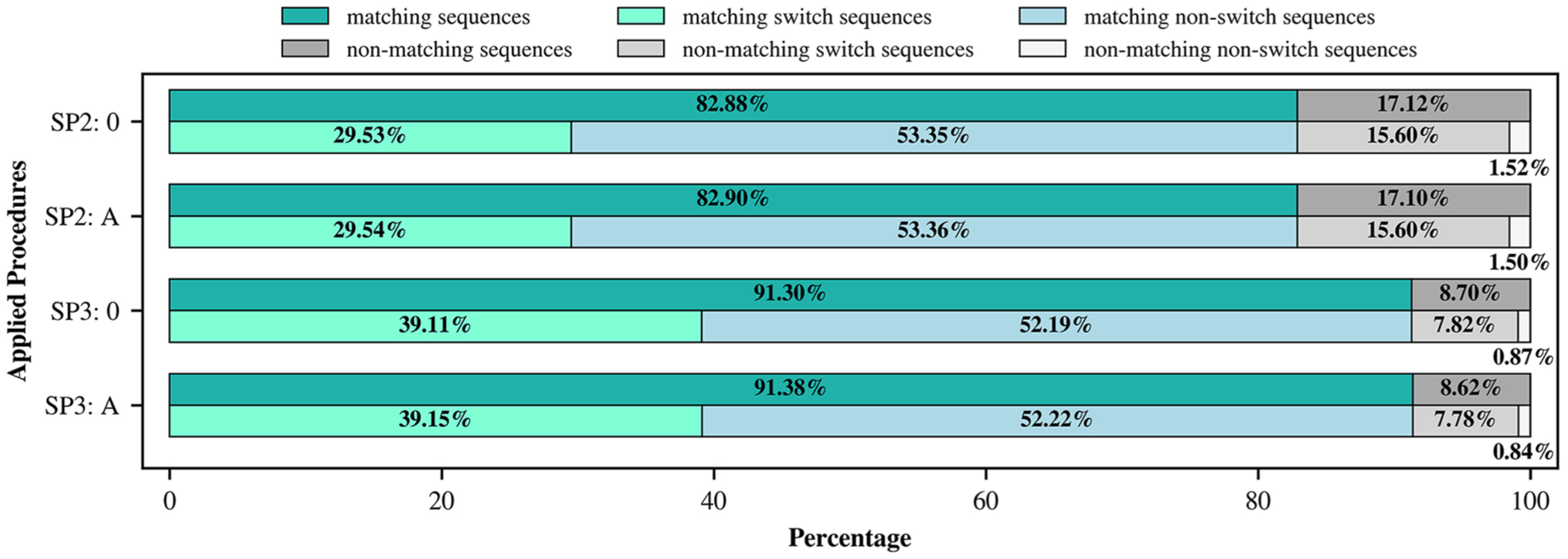
Accuracy of the predicted MT-signal state sequences for Intersection 002.
The derived, respectively predicted signalization sequences contain up to three signal changes. For SP2, applying the baseline case provided a PPV of 95.66% and a TPR of 93.67% (Table 2). This means that, on average, 9,566 of 10,000 predicted signal changes occur in the ground truth, and only 633 of 10,000 SC of the ground truth were not derivable in the predicted signal state sequences. For the T2SC predictions of actual signal changes included in the signal state sequences of the next 30 s, an MAE of 1.02 s and an RMSE of 2.68 s were obtained. In comparison, Procedure A provided a slightly higher PPV measure of 95.71%, a marginally lower TPR value of 93.66%, the same average MAE value of 1.02 s, and a slightly lower RMSE value of 2.67s. For periods during SP3’s active time, such as for the achieved ACC values, applying Procedure A only provides slightly higher improvements. Nevertheless, a higher prediction quality can be deduced for those periods compared with non-peak hour periods. This is because of the higher densities and volumes during peak traffic conditions, which lead to more regular and in some cases almost continuous detector actuations at the intersection. In such scenarios, traffic-actuated signal control often converges toward fixed-time-like behavior by repeatedly switching the same patterns until the demand situation at the intersection changes. Consequently, this switching behavior reduces the variability in signal timing and increases the predictability of switching patterns.
Obtained Quality Measures for Signal Change Predictions for Intersection 002
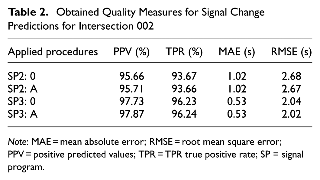
Note: MAE = mean absolute error; RMSE = root mean square error; PPV = positive predicted values; TPR = TPR true positive rate; SP = signal program.
The differences between the RMSE and MAE values primarily result from the presence of a small number of larger deviating T2SC predictions, which have a disproportional strong impact on the RMSE because of its quadratic error term. These often occur in cases where a detector actuation that triggers one or more switching events has not yet happened at the time of prediction. Because new T2SC predictions are generated every second, these late-occurring events can lead to several temporally distant and inaccurate predictions being made before the system behavior becomes predictable with the existing feature scope. Most predicted switching times exhibit low deviations, but some predictions show distinctly higher deviations. This results in a right-skewed error distribution, where most predictions cluster around low error values, but a long tail of larger errors remains. This distribution pattern is reflected in the cumulative error distribution (CED) plot (see Figure 8), where a steep rise in the lower error ranges is followed by a flattened tail.
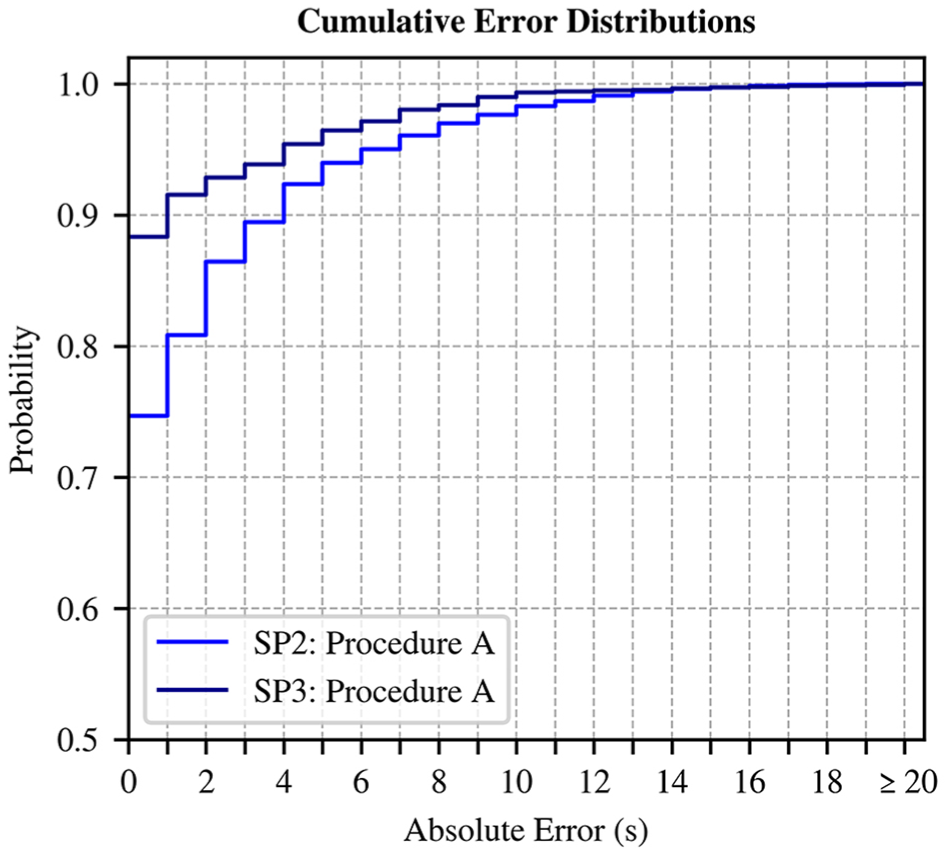
Cumulative error distribution of T2SC predictions by Procedure A for Intersection 002.
Overall, the application of Procedure A only provided minor enhancements. The space for potential improvements could be expected to be small if the developed procedure is applied in combination with well-generalized predictive models. In this context, the obtained results indicate that the applied predictive models are well-generalized, up to the degree that they only output very few detectable implausible predictions. This assumption is further supported by the results obtained for applying Procedure B, which only resulted in the adjustment of a few thousand predicted signal state sequences of the next 30 s compared with the about 10 million predicted sequences. As a result, improvements were only determined in higher decimal place ranges of the applied evaluation metrics. Therefore, no appreciable performance gain could be deduced either for the bare application of Procedure B or for the subsequent application of Procedure B (A + B). However, the small number of adjustments indicates that most derived signal state sequences pass the incorporated plausibility tests. Therefore, even if no distinct increased prediction accuracy was achieved, the application of Procedure B further shows that nearly no predictions that violate green permission periods or do not comply with the permitted green durations were made.
Deducing, however, whether predictive models are well-generalized or not based solely on obtained evaluation metrics can be a challenging task. As such, applying the developed procedures has been shown to be beneficial, as they provide a comparison case. This is further exemplified in Table 3, which presents the results of additional experiments conducted for the same train and test data splits of SP2. The models, however, were trained with less optimized sets of hyperparameters. For the baseline case, an accuracy for the signal state sequence predictions of 80.67% was obtained. In contrast, Procedure A provided an enhanced ACC of 82.74%, indicating that a share of implausible predictions were made by applying the baseline prediction procedure. However, the ACC values obtained for Procedure A come close to the achieved accuracies presented in Figure 6. The same applies to the obtained PPV of 95.22%, TPR of 93.9%, and the obtained average MAE and RMSE values of 1.01 and 2.64 s (Table 3).
Prediction Quality Measures Obtained by Less Generalized Predictive Models
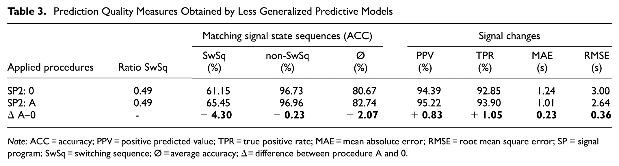
Note: ACC = accuracy; PPV = positive predicted value; TPR = true positive rate; MAE = mean absolute error; RMSE = root mean square error; SP = signal program; SwSq = switching sequence; Ø = average accuracy; Δ = difference between procedure A and 0.
Figure 9 shows the CED and differences in error shares between the suboptimal baseline case and Procedure A. Procedure A provided a higher share of T2SC values predicted with no or only minor deviations (Figure 9). At the same time, the share of T2SC predictions with higher temporal deviance from the actual switch time is lower (Figure 9, a and b ). Given the symmetric percentage differences in the error shares, the proportion of inaccurate T2SC predictions is distinctly lower for Procedure A; at the same time, the proportion of predictions with no or only slight temporal deviations is greater (Figure 9c). In the context of Figure 9c, symmetric differences were used to account for unequal total prediction counts, as Procedure A predicts a slightly higher number of actual signal changes.
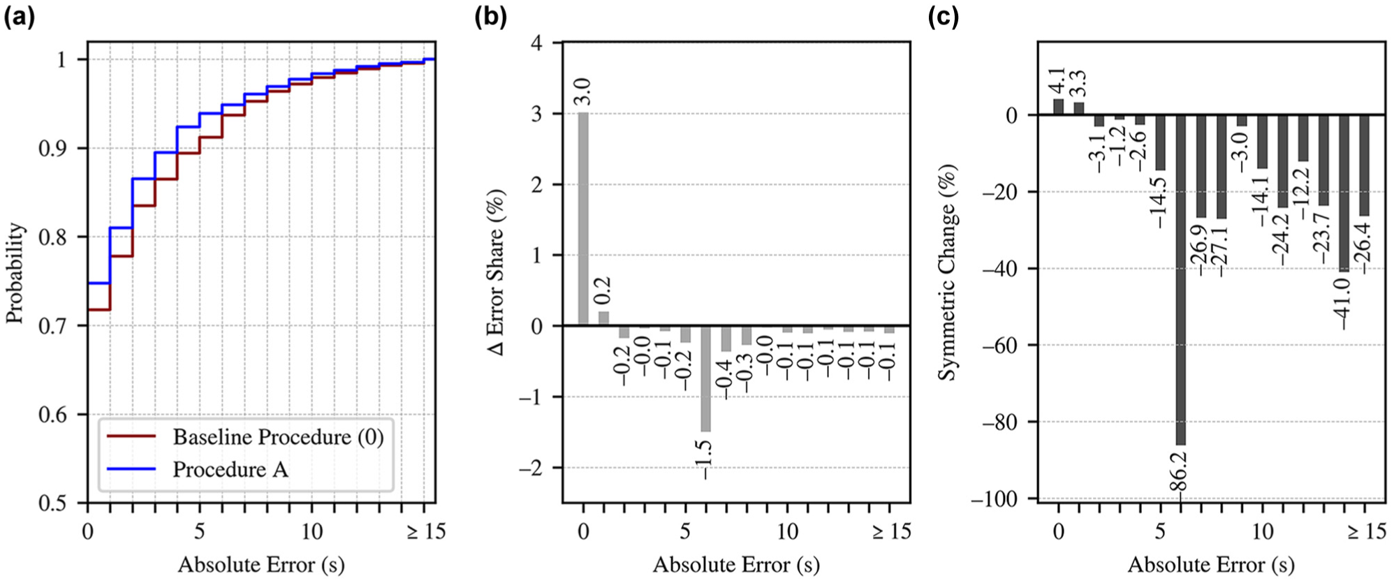
(a) Cumulative error distribution; (b) absolute; and (c) symmetric percentage differences in error share by error class of T2SC predictions between the suboptimal baseline case (0) and Procedure A (Intersection 002 SP2).
Overall, the application of Procedure A, combined with the less generalized models, provided an enhanced prediction quality, as deduced by the improvements in every considered evaluation metric (Table 3) and based on the lower rates of inaccurate T2SC predictions (Figure 9). Furthermore, the gap between the prediction quality achieved by well-generalized models compared with less generalized models appears to be reduced because of the application of Procedure A (see Figure 7 and Tables 2 and 3). These results show the potential of the incorporated methods for preventing, identifying, and adjusting implausible predictions, for enhancing, respectively, securing a decent degree of accuracy, if they are applied to less generalized predictive models. Furthermore, a notable reduction can be observed in the 6-s error class, showing an absolute change of 1.5% and a symmetric reduction of over 85% (Figure 9, b and c ), which are distinctly higher than those in the neighboring classes. This pattern may point to the limited generalization capabilities of the less-tuned predictive models used in the baseline case, leading to a higher share of implausible predictions. Considering this, a comparison between the application and non-application of Procedure A may also help to identify insufficiently generalized models.
Results Obtained for Additional Intersections
Additional experiments were conducted to determine whether the previous findings also apply when the procedures for identifying and adjusting implausible predictions are applied at other intersections. For these experiments, historical data from three additional intersections of our data stock were utilized. Those intersections are located near Intersection 002 in the city of Kassel (Germany) and are controlled traffic-actuated with a fixed cycle duration as well.
For these experiments, the same train, test, and validation data splitting procedure as in Intersection 002 was applied. To obtain the constraints-dictionaries (required for the application of prediction Procedure A).
Figure 4 shows the specific analysis scripts that were applied to the additional intersections training data. Furthermore, similar to the previous experiments, two test series were considered. For the first series, the hyperparameters for each model were tuned beforehand; for the second series, less well-generalized models are “simulated” using a set of less optimized hyperparameters for the model training.
Table 4 summarizes the results for the experiment series involving the predictive models for which the hyperparameters were tuned individually. Therefore, the summarized results represent values averaged over all intersections. Overall, as for the experiments for Intersection 002, Procedure A’s application provided a slightly higher prediction quality than the baseline procedure. Except for the average TPR value for the prediction experiments conducted for periods of the daytime outside peak hours (SP2), which is the same up to the third decimal place, Procedure A’s slight improvements can be determined for each evaluation metric considered (see Table 4). For predictions made for peak hour periods during the active time of SP3, an improvement in each evaluation metric because of Procedure A was achieved (Table 4).
Obtained Prediction Quality Measures, Averaged Over All Three Additional Intersections
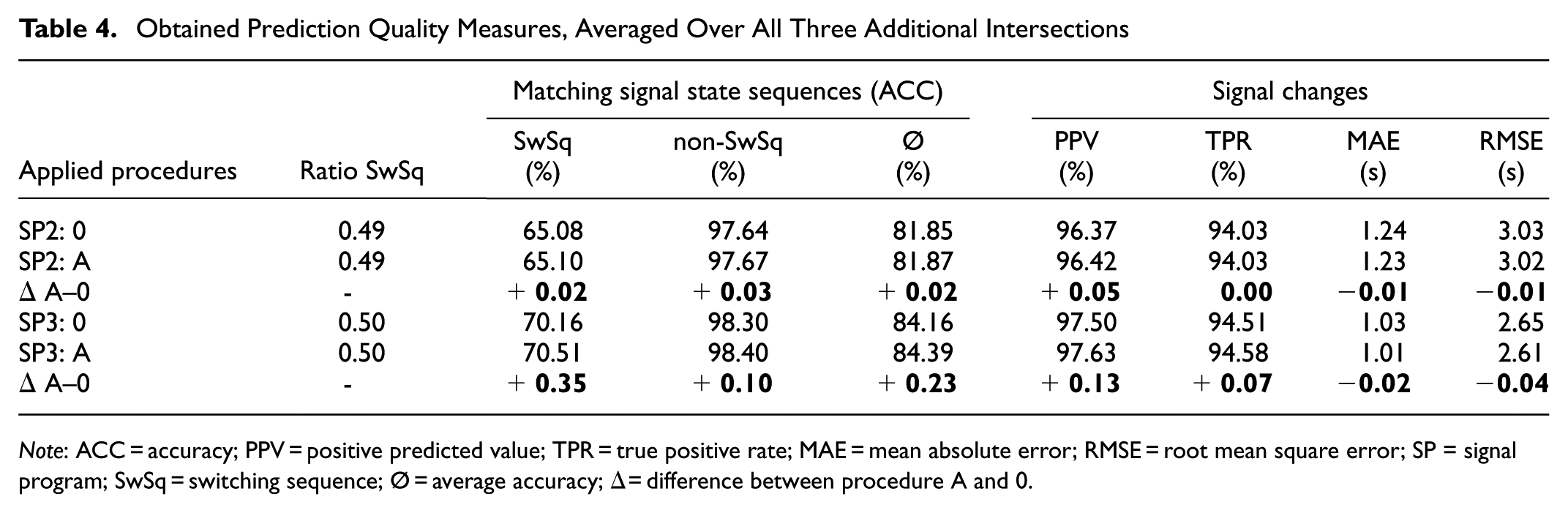
Note: ACC = accuracy; PPV = positive predicted value; TPR = true positive rate; MAE = mean absolute error; RMSE = root mean square error; SP = signal program; SwSq = switching sequence; Ø = average accuracy; Δ = difference between procedure A and 0.
In relation to the temporal deviation in the SC predictions, the application of Procedure A provided a slightly lower mean average error for the data of both SP (Table 4). Figure 10 shows the CED of the predicted T2SC values for the models with individually tuned hyperparameters. Based on the only slightly reduced MAE and RMSE values (Table 4), the differences between the baseline procedure and Procedure A are generally small. For SP2 (Figure 10a), the curves are nearly identical, with deviations between both procedures remaining in the range of a few tenths of a percentage point. For SP3 (Figure 10b), which covers T2SC predictions made for peak hour periods, Procedure A leads to a slightly more noticeable leftward curve shift.
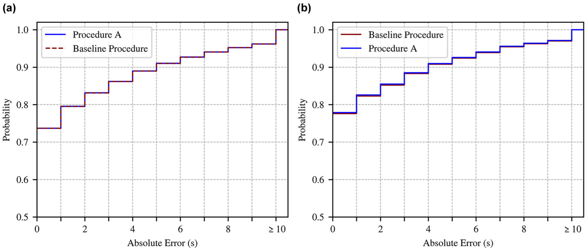
Cumulative error distribution for T2SC predictions for periods of the operation times of: (a) SP2; and (b) SP3, measured over all three additional intersections.
The results of the experiment series involving the less generalized predictive models are summarized in Table 5. For this scenario, similar to the results for Intersection 002 (Table 3), the application of Procedure A provided distinct enhancements for any considered evaluation measure.
Prediction Quality Measures Averaged Over All Three Additional Intersections Obtained By Less Generalized Predictive Models
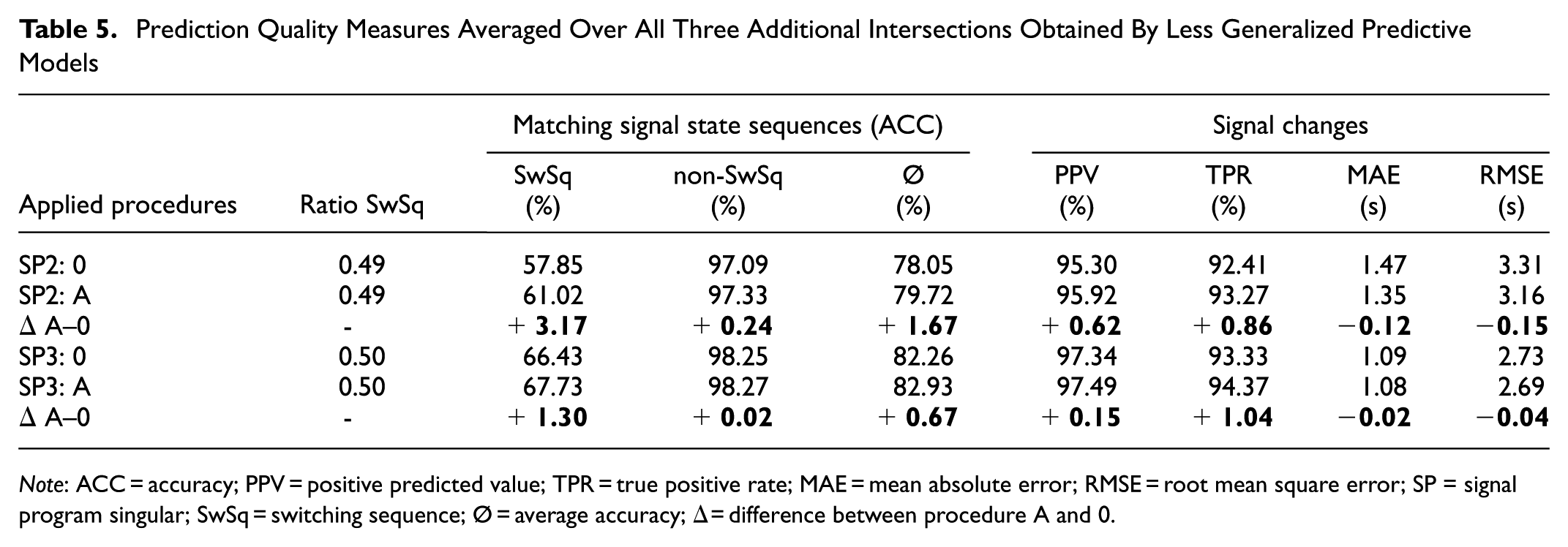
Note: ACC = accuracy; PPV = positive predicted value; TPR = true positive rate; MAE = mean absolute error; RMSE = root mean square error; SP = signal program singular; SwSq = switching sequence; Ø = average accuracy; Δ = difference between procedure A and 0.
Figure 11 shows the CED ( a and b ) and differences in error shares ( c and d ) of the T2SC predictions made for SP2 and SP3, based on the less-tuned predictive models. For both signal programs, Procedure A leads to a slightly higher share of T2SC predictions with low absolute deviations, whereby this effect is more pronounced for SP2 (Figure 11, c and d ). This corresponds to the slightly higher improvements in MAE and RMSE listed in Table 5. Applying Procedure A increases the share of low error T2SC predictions for SP2; this trend is less pronounced for SP3. In this case, although a reduction of large deviations is still visible, the improvements do not consistently result in error-free predictions. Instead, a portion of the adjusted predictions shifts into medium-range error classes, suggesting that procedure A mitigates implausible outliers but does not always yield precise corrections to the actual switching time. Although the predictive models used here were trained with less optimized hyperparameters, they may still have generalized better, in relation to providing plausible predictions, than the predictive models applied for intersection 002, as suggested by the overall narrower gaps between the baseline procedure and procedure A.
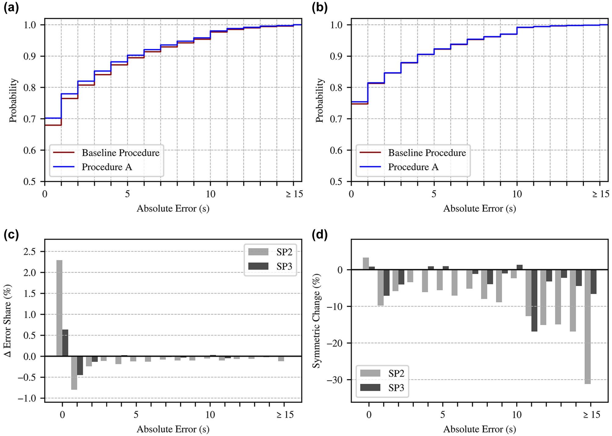
(a and b) Cumulative error distribution; (c) absolute; and (d) symmetric percentage differences in error share by error class of T2SC predictions between the suboptimal baseline case (0) and Procedure A for periods of the operation times of (a) SP2 and (b) SP3 measured over all three additional intersections.
In summary, the results obtained for the additional intersections match the findings determined based on the results achieved for Intersection 002. In cases where the predictive models are trained with finely tuned hyperparameters and, therefore, are likely to be well-generalized (up to a certain degree), the developed procedures for identifying and adjusting implausible switching time predictions provide prediction quality improvement with a small magnitude. In cases where predictive models are less generalized, the developed procedures display the potential for enhancing or securing a decent degree of prediction accuracy. Therefore, the showcased potential provided by the developed procedures appears to be beneficial in relation to slight improvements in the prediction quality and can also help to determine whether models are well-generalized based on the magnitude of quality improvement.
A high magnitude of improvements indicates that the predictive models are less well-generalized. On the other hand, a low magnitude indicates that the predictive models might be well-generalized in relation to not providing a high share of implausible predictions, which violate, for example, permissive periods of certain MTSSt or which violate allowed switching sequences. However, it is beyond the capabilities of the applied procedure to ensure entirely correct predictions. Implausible predictions account for only a subset of all incorrect predictions. As described previously, a certain share of incorrect predictions arises from limited information about future green time requests available at the prediction time. Consequently, detecting and correcting implausible predictions can only improve a limited portion of the overall prediction error.
Conclusions
The targeted additional consideration of boundary conditions, causalities, and relations in the switching behavior of a traffic-actuated signal system, combined with an ML-based prediction approach, is valuable for evaluating the plausibility of made switching time predictions. The results of the plausibility tests enabled further conclusions relating to the generalization of the applied predictive ML models. Applying the procedures developed to prevent, identify, and adjust implausible outputs of the applied predictive model has proven valuable, especially when they are applied to less generalized predictive models.
This study presented a methodology consisting of data preparation, developing, and applying procedures for preventing, identifying, and adjusting implausible predictions of the future signalization of traffic-actuated signals, and testing and comparing the performance of different combined application cases of those procedures. The framework, incorporating the different considered application cases, was first applied to the historical data of a selected four-way traffic-actuated signalized intersection. One adjustment procedure was shaped to the applied MTSSt-oriented prediction approach, and another was considered for a targeted adjustment of (derived) implausible predicted RTs until a signal status changes.
The results, which were further supported by conducting additional experiments with historical data from three other traffic-actuated controlled signal systems, show that applying both procedures can contribute to evaluating the generalization of applied ML models. If applied in combination with well-generalized models, the procedure, shaped to the applied MTSSt-oriented prediction approach, provided minor enhancements of the achieved accuracy of the switching time predictions. However, when applied in combination with less generalized models, a visibly enhanced accuracy of the predictions compared with the bare application of these models was obtained overall and for every considered traffic signal system. The achieved accuracy even reaches the same magnitude as that of the combined application with well-generalized models when measured by the applied evaluation metrics, in certain cases.
This shows the potential of the incorporated methods for preventing, identifying, and adjusting implausible predictions, for enhancing or securing a decent degree of accuracy, even if they are applied to less generalized predictive models. This further allows the assumption that the developed procedures could contribute to ensuring a decent degree of prediction accuracy if special events occur, which may weaken the reliability of an applied prediction model, such as unusual traffic situations or failures in the data acquisition of detectors.
However, overall, the magnitude of the achievable performance benefit of these procedures, which incorporate evaluating the plausibility of made predictions, depends on the generalization of the ML model. In addition, it is beyond the capabilities of the applied procedure to ensure that only correct predictions are made. Especially for switches further in the future, a lack of information relating to the future occurrence of these switches, such as future detector actuation, becomes the bottleneck and a more crucial factor than implausible predictions, limiting the achievable forecast accuracy. To exemplify, a predictive model, which is making predictions based on current feature measures, is lacking information to properly predict an SC that will occur 30 s in the future when this SC is triggered by a detector that will be actuated itself in 20 s. However, this lack of information can theoretically be closed to a certain degree by incorporating predictions of future detector actuation, especially actuations by vehicles. This is one aspect that our future research will focus on.
Nevertheless, based on the results of the prediction experiments conducted with the data from different traffic-actuated signal systems, this study has shown that incorporating plausibility tests in an ML-based STF approach can be worthwhile. To the best of our knowledge, this study is the first work in the field of STF in which an ML-based approach was combined with plausibility checking to identify and adjust implausible predictions. The presented findings may encourage other researchers to consider incorporating similar procedures tailored to their approaches, aiming for a potentially (slightly) increased accuracy of their switching time predictions, and as a tool for evaluating the generalization of their applied ML models. In this context, given that the controller logic is available, boundaries that are further than those identified by the statistical analysis of the historical data could be considered, allowing more precise plausibility tests and adjustments to identified implausible predictions.
Footnotes
Acknowledgements
We thank the City of Kassel for providing the data. We further acknowledge the support of Deutsche Forschungsgemeinschaft (DFG).
Author Contributions
The authors confirm contribution to the paper as follows: study conception and design: Heckmann, Budde; data collection: Heckmann; analysis and interpretation of results: Heckmann, Budde, Hoyer; draft manuscript preparation: Heckmann, Budde, Hoyer. All authors reviewed the results and approved the final version of the manuscript.
Declaration of Conflicting Interests
The author(s) declared no potential conflicts of interest with respect to the research, authorship, and/or publication of this article.
Funding
The author(s) disclosed receipt of the following financial support for the research, authorship, and/or publication of this article: This research was supported by Deutsche Forschungsgemeinschaft (grant no. 461855625).