Predicting the Future Signalization of Traffic-Actuated Signals Using Extreme Gradient Boosting

Abstract

Stops, braking, and acceleration maneuvers at traffic signals cause high fuel consumption and emission levels. Green light optimized speed advisory (GLOSA) can help to reduce a proportion of such unnecessary vehicle maneuvers. For this, GLOSA systems require reliable switching time estimations as input. However, estimating the switching times of traffic-actuated signals can be challenging. The signalization of traffic-actuated lights is adjusted to match the current traffic. Based on green-time requests, the status of signals can change with almost no lead time. This paper presents an approach for predicting the signalization of traffic-actuated signals. We exploit the limited nature of the space for switched signal state combinations at intersections, and express combinations of motorized traffic-related signal states as one feature to depict the motorized traffic signalization state (MTSSt) at an intersection. Predicting MTSSt-switches allows later determination of the switching times of individual signals. To conduct the predictions, the machine learning method “extreme gradient boosting” was used. A three-step methodology—data preparation, tuning the prediction procedure, and testing the approach—was applied and evaluated on the historical data of four traffic-actuated signalized intersections. The results showed that within a period of the next 30 s, signal changes were predicted with an overall precision and sensitivity of about 95% and an average mean absolute error of less than 1.1 s. In this period, the sequence of switched signals was predicted accurately to the second, without any deviation, in, on average, over 82% of cases.

In urban areas especially, traffic signals have an impact on fuel consumption and greenhouse gas emissions. Reducing unnecessary stops, braking, and acceleration at traffic signals can help to save fuel and to reduce emissions. In areas with closely spaced intersections, a proportion of unnecessary stops could be avoided by setting up coordinated signal timing to create an uninterrupted traffic flow.

Cooperative intelligent transport systems applications, such as green light optimized speed advisory (GLOSA) systems, offer a further approach. Independent of the distances between intersections, GLOSA, and similar ecodrive applications, provide drivers—human or (semi)autonomous—with strategies such as speed recommendations, to avoid unnecessary braking, stopping, and accelerating before traffic signals. When used for generating speed recommendations, these applications incorporate information about the near future signalization of traffic signals.

In addition, certain bidirectional vehicle to infrastructure (V2I) and infrastructure to vehicle communication approaches have been proposed ( 1 – 4 ). Based on transmitted or detected vehicle positions and speeds, such approaches, often referred to as ecosignal approaches, aim to simultaneously optimize the driving of approaching vehicles and traffic signal timings. However, currently, most ecosignal studies assume high market penetration rates (MPRs) of autonomous or connected vehicles (CVs) and/or are evaluated under isolated simplified conditions, for example, a limited degree of freedom for lane changes or failing to consider the potentially disruptive influence of pedestrian green-time requests. As concluded by Ko et al., further investigations into the effects of ecosignals are required ( 2 ). Considering these challenges, optimizing the driving of individual vehicles or sole platoons appears to be more practical at present.

The scope of the research addressing the development and evaluation of GLOSA, or similar ecodrive algorithms, covers various approaches. For example, Asadi et al. proposed an algorithm that uses upcoming traffic signal information within the vehicle’s adaptive cruise control system to reduce idle time at stop lights and fuel consumption ( 5 ). Similar approaches for platoon cases and/or (semi)autonomous vehicles can be found ( 6 – 11 ). Reinforcement learning-based approaches for ecodriving in the vicinity of signalized intersections have been presented ( 12 – 14 ). Dabiri et al. propose optimal speed advice for cyclists to increase the success rate of catching green lights ( 15 ), which indicates that providing speed advice is not beneficial exclusively for motorized vehicles.

In addition to the aforementioned research, the potential contribution of GLOSA and similar ecodrive applications to reductions in vehicle fuel or electric power consumption, emissions, and waiting times has also been demonstrated in various research ( 16 – 24 ). However, in most GLOSA/ecodrive studies, signalization of the traffic signal system is or is assumed to be pretime controlled, or respectively, the future signalization—a crucial input for optimizing driving strategies—is assumed to be known. In the scope of a GLOSA mapping study, Mellegård et al. pointed out that only a few research studies consider traffic-actuated signal systems, which are most prevalent in urban areas where GLOSA is expected to be most effective ( 25 ).

In Germany, for example, most traffic signals are already operated as traffic-actuated ( 26 ), and an increase in the usage of traffic-actuated control is expected worldwide ( 27 ). Favoring an optimized traffic flow, the signalization of traffic-actuated signals is adjusted to match the current traffic: parameters relating to the current traffic at the intersection area are used—gathered with the help of detectors. Depending on the respective signal program (SP) of a traffic-actuated signalized intersection, the duration and the sequence of phases can be adjusted, and signal states can change with almost no lead time. Since these control decisions depend on current traffic volumes, traffic signal controllers are unable to forecast their own behavior. Furthermore, actuated green times cannot be accurately estimated from historical statistics, even under the same traffic conditions ( 28 , 30 ).

Consequently, as concluded by Mellegård and Reichenberg ( 25 ), and Stevanovic et al. ( 28 , 29 ), the benefits of GLOSA (for actuated signals) cannot be utilized until a way is found to provide accurate estimates of phase durations and switching times (STs). Thus, to utilize the benefits, and enable the widespread use of GLOSA and similar ecodriving or red-light violation warning (RLVW) systems, switching time forecasts (STFs) for traffic-actuated signals are crucial to provide accurate information about the signalization of traffic-actuated signal systems ( 31 ). Information about traffic signals’ current and future signalization is also requested as input for routing applications ( 32 , 33 ).

Most studies dedicated to STFs of traffic-actuated signals focus on predicting either the remaining time until the next change from red to green (time to green [T2G]) or the remaining time until the next signal change (T2SC). In T2G approaches, predictions are usually only made if the current state of a signal is red. As the (remaining) duration of green time (which could further be actuated by traffic) is a decisive factor in whether an intersection can or cannot be passed without stopping, these approaches do not provide information that can help drivers or autonomous cars, to adapt their driving during green periods. However, T2SC approaches can be utilized to predict either the remaining T2G or -time to red (T2R), depending on the current state of a signal (red/green), by providing information about how long the current signal might remain either green or red. Nevertheless, the period for which T2SC approaches can offer information about future signalizations is limited to the time until the next signal change (SC). This prediction horizon inevitably gets smaller the closer in time the next switch is, and then increases abruptly with the occurrence of the next switch. This also applies to T2G approaches.

Because of the inconstant prediction horizon of the next SC, these approaches lack the information that would allow the reliable optimization of driving strategies for vehicles that are at a greater distance from a signalized intersection. To address this lack and provide a sufficient period in advance for which information about the future signalization of traffic-actuated signals is available, more than the very next switch must be predicted with reasonable accuracy.

To ensure traffic safety at signalized intersections, the states of signals are interdependent. Based on defined rules, the signal control unit determines each connected signal’s state and STs, always ensuring that the overall intersection’s signalization remains in a state that provides traffic safety. The overall state of signalization at a point in time can therefore be considered a combination of the current state of each intersection’s signal (see Figure 1). Thus, the future states and STs of each signal can be determined by prediction of the general signalization of an intersection. However, pedestrians and public transport (PT) vehicles are often released on request and are not the potential primary users of either GLOSA or smart routing applications. In this context, determination of the STs of these user groups can be omitted. Therefore, a prediction task can be refined to predicting motorized traffic-related signals only. As shown in Figure 1, the signalization of motorized traffic-related signals can be expressed at the level of (general) motorized traffic signalization states (MTSSts). Because of the operational and temporal restrictions set in the control unit, the space for switched MTSSts and the space for allowed sequences in which these states can succeed one another is limited.

Figure 1.

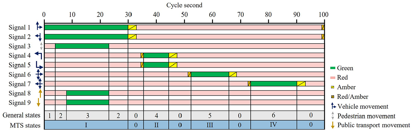
Signal timing plan and general states/motorized traffic signalization state (MTSSt) definitions.

Following this idea, this paper presents an approach for predicting the future signalization of traffic-actuated signals based on predicting switches of MTSSts using machine learning (ML). The underlying assumption of this approach is that the impact of factors (e.g., green-time requests of pedestrians and PT, defined temporal dependencies), which pose major challenges for STFs, can be mapped more easily by a predictive ML model on this small state space. To this end, data from vehicle- and pedestrian detectors and information about approaching PT vehicles were instrumental in training the predictive models.

Unlike studies that focus on predicting the time until the next green or red switch (of single signals), the current research predicted several MTSSt-switches in advance. According to Tielert et al., the benefit of providing approaching strategies reaches a saturation point at about 500 m before an intersection ( 19 ). The same margin of approximately 500 m before an intersection was also indicated by the results of Ala et al.: a 500-m control segment provided the greatest fuel consumption savings ( 6 ). Therefore, to theoretically exploit the maximum benefit of GLOSA, this approach was tuned to constantly provide information about future signalization for a horizon of at least 30 s in advance. A sufficient number of MTSSt-switches in advance was predicted to ensure this horizon was always reached. As a result of this, the approach further provided estimates for more than one SC in advance and overcame the “converging to 0” flaw, before the prediction horizon abruptly “jumping.” To predict the MTSSt-switches, the ML method extreme gradient boosting (XGBoost) was used ( 34 ). The presented approach is designed to be extendable from its reliance on historical data, and is theoretically applicable at any signalized intersection, regardless of the type of signal control. This research had two main objectives, to

1. Outline a framework for predicting MTSSt-switches and determine future switches of single signals based on these predictions; and

2. Test the framework using historical field data of several traffic-actuated signalized intersections.

The remainder of this paper is organized as follows: the literature review briefly discusses the related works in the field of STFs; the subsequent section presents the methodology of the approach; the succeeding section presents and discusses the results of the field studies; and the last section concludes this paper.

For the sake of simplicity, the abbreviation MT will be used to refer to motorized traffic hereafter. In addition, signals used to signalize MT will be referred to as MT-signals.

Literature Review

Some approaches dealing with STFs use floating car data as the primary input data source ( 35 , 36 ). However, since these approaches do not involve parameters gathered by detectors, they cannot map the reactivity of traffic-actuated signal controls to changing traffic situations. Therefore, they are only suitable for pretimed traffic signals, as are the approaches that use only (historical) process data ( 37 – 40 ). Especially if certain phases are only switched if they are requested, and when green times can vary sufficiently in their length and position in the cycles, historical statistics of STs alone (i.e., not linked with further conditions) are insufficient to provide accurate estimates.

Bauer et al. proposed that the future switching behavior of traffic-actuated signals could be predicted by applying a digital twin (emulator) of the signal controller ( 41 ). In practice, signal control logic is usually iterated secondwise, using current detector information, to decide whether a signal will remain in its current state or if the state is going to change. As a result, multiple iterations ahead of the current time must be emulated to cover a decent prediction horizon. Thereby, to provide reliable emulation results, changing input conditions like future detector activity must be anticipated (respectively estimated) with a high level of confidence in both the assumed actuation state and the temporal occurrence. In an ideal scenario, an environment consisting exclusively of CVs, route choices, vehicle positions, and speeds could be transmitted, allowing accurate predictions of future request/actuation scenarios. Regardless of whether such an ideal scenario will become a reality in the (near) future, and in addition to the requirement of available digital twins, challenges arise in relation to accurately determining approaching vehicles/platoons, their route choices, speeds, and arrival times under the current conditions in the field, where MPRs of CVs are currently low. Mousa et al. proposed the installation of additional detectors located upstream of minor approaches to estimate arrivals at intersections ( 42 ). Even though the results of Mousa et al. indicate decent effectiveness for enhancing the quality of estimated red indications on the major road approaches, such an approach requires investment to install additional detectors ( 42 ). Furthermore, lane changes downstream of the additional detectors, especially in relation to turning lanes, still require estimation.

Most of the recent research on STFs of traffic-actuated signals aims to predict future signalization by applying ML algorithms for training predictive models. For this, historical data from traffic signals, including detector data, are used. Unlike emulators, which may require several iterations before a future switching event can be derived, these models are trained to directly predict certain switching events based on (current) input data.

Weisheit used support vector machines to predict the STs of traffic-actuated signals ( 43 ), whereas Genser et al. compared the performance of three different ML methods to predict the T2G of several signals at an intersection in Zurich (Switzerland) ( 44 ). In our performance comparison, we considered 12 different ML methods (e.g., support vector machines), including random forest, XGBoost, and recurrent neural networks to predict the T2G and the T2R at two intersections. In this study, XGBoost provided the best results ( 45 ).

Eteifa et al. describe a long short-term memory neural network-based approach applied to the historical data of a four-way intersection in Merrifield, VA; this implemented a coordinated traffic-actuated signal operated by a six-phase National Electrical Manufacturers Association (NEMA) signal controller ( 46 ). The authors compared different loss functions for training predictive models to predict the T2G and the T2R of signal phases. For a horizon between 0 and 20 s until an SC, one model reached a mean absolute error (MAE) of below 2 s. Whether the results achieved by Eteifa et al. for the selected intersection could be transferred to traffic signal systems that are controlled in a more complex way (e.g., also offering prioritized releases for PT vehicles), should be reviewed ( 46 ).

Certain approaches aim to predict signalization of traffic-actuated signals using a stage-oriented operated signal control, the predominant type of signal control in Germany ( 47 – 49 ). Bodenheimer et al. presented a graph-based Bayesian approach to predict the time until a signal changes based on previous predictions of the next transition ( 47 ). In a previous study, by predicting stages and transitions, we addressed how, in some cases, stages can follow each other without an intermediate transition ( 49 ). However, the scope of stage-oriented approaches is limited, as not every intersection’s signalization is controlled in a stage-oriented manner. Another disadvantage of stage-oriented approaches, in general, is that information about the stages and transitions defined in the signal control program is required. Therefore, this information must be available in the process data, which is often not the case, or it must be derived using external information or expert knowledge.

In a further study, we presented an ML-based approach to predict traffic-actuated signals by predicting sequences of general states of signalization ( 50 ); to the best of the authors’ knowledge, this was the first time that data on approaching prioritized PT vehicles were used in an STF-related approach. However, because we initially intended using general state predictions only as additional input to improve the accuracy of T2G and T2R predictions of single signals, determination of single signal switches was omitted ( 50 ).

The current study builds on the findings of our previous approach, involves enhancements in relation to the used ML methods and selected features, and determines the STs of MT-related signals. By focusing on providing STFs for the primary user group of GLOSA, specifically, and of cooperative applications in general, participants of the MT, this approach overcomes the flaws in our earlier work ( 50 ). Because of the significantly lower number of distinct switched MTSSt than the number of unique general states, it was less computationally expensive and provided higher accuracy for larger prediction horizons.

Methodology

A three-step methodology was used to predict signalization of traffic-actuated signals. In the first step, historical data of real-world traffic signal systems were prepared to train ML models for predicting MTSSt-switches. This step involved analyzing and formatting the logged raw data to extract valuable features for the given prediction task and obtaining target variables for the application of supervised learning.

The second step involved developing a prediction procedure, which included the selection and tuning of suitable ML methods and a procedure for determining the signalization of MT-signals based on MTSSt-switch predictions. The final step was testing the approach by conducting field studies based on historical data.

Data Preparation

The stock of historical data used for developing and evaluating the presented STF approach were provided by City of Kassel’s local urban traffic and roads authority, Germany. The provided raw data consisted of daily log files from multiple signalized intersections within the city area. These logfiles essentially contain the cycle seconds and timestamps of signal switches and the state changes of vehicle and pedestrian detectors. When priority is given to PT, announcements from PT vehicles are also included. A Python script was used for preprocessing and converting the raw data into a data frame structure.

Firstly, all relevant data were extracted. Then, the gaps between the logged state changes of the signal heads and detectors were logically filled. Periods for which no data were available for detectors and signal heads were removed. The data of signal heads that only display hazard warnings were also removed, as these signals have no impact on control decisions and are therefore of no benefit to STFs. The signal heads that always display the same signal were arranged into signal groups (SGs).

The German guidelines for traffic signals (RiLSA) refers to an SG as “one or more signal heads that control specific traffic streams and show the same signal at any given time” ( 51 ). This generally results in the expression of multiple signal heads, controlling the same traffic stream(s) as one signal group, for example, if multiple lanes are provided for those streams or if, to facilitate better visibility, multiple signal heads at differing heights or locations are set up.

For each SP of each intersection, the processed raw data were then aggregated on a monthly basis and merged secondwise to create initial data models that contained the following features for each second of data:

• Minutes since midnight (float value),

• Current cycle second,

• Current signal state of each signal group, and

• Current state of each detector.

To reduce the value range and unify the signals shown for the different road user groups (pedestrians, MT, and PT), the SG states only differentiated between displayed signals representing “a release” or “no release.” If priority was given to PT at the intersection, the recorded messages from the PT vehicles were preprocessed in a separate step and merged with the initial data models. Three notification points (NPs) were established along each approaching road to prioritize PT at specific intersections in Kassel, forming a notification chain.

The furthest NP was used for the preregistration of PT vehicles, the next for the main registration, and the third for deregistration when the PT vehicles passed the intersection. Every time a PT vehicle passed an NP, it sent a message to the downstream traffic signal controller. This message contained, among other information, the route ID on which the PT vehicle was traveling. Based on information in the technical documentation of intersections provided to us, along with the logged raw data, the route IDs were linked with the SGs that released the vehicles operating on specific routes. This way, the request states of the individual PT-related SGs were determined and merged with the initial data models.

Since the raw data did not contain information about the switched MTSSts, this key feature had to first be derived, as did the target features of the approach: the future MTSSt-switches. These target features comprise the future switched signalization states of MT ( $\mathrm{MTSS}{t}_{+1},\dots ,\mathrm{MTSS}{t}_{+n}$ ), and the residual times until these states are switched ( $R{T}_{+1},\dots ,R{T}_{+n}$ ). By combining the predicted states with their corresponding predicted residual times, the future signalization of MT-signals can be determined.

To obtain the required MTSSts and target features for every second, k, included in the initial data models, an adapted version of the procedure described by Hoyer et al. ( 52 ) was used (see Figure 2). In the first step, a MT signalization vector, $\underset{¯}{\mathrm{mv}}\left(k\right)$ , was generated. This vector contains the individual state of each MT-related SG at second k, only distinguishing between the binary states green ( = 1) and not green ( = 0). By calculating the scalar product of $\underset{¯}{\mathrm{mv}}\left(k\right)$ and a transformation vector, $\underset{¯}{\mathrm{tv}}$ , an integer value is obtained. This value, $\mathrm{MTSSt}(k)$ , represents an identifier, expressing the current state of the signalization of MT at the intersection at that specific time. Based on the shape of $\underset{¯}{\mathrm{tv}}$ , these MTSSt values are unique for each unique state of MT signalization. By calculating the MTSSt values for each second of the data, the MT signalization sequence was obtained. Subsequently, the target variables were determined based on the temporal evaluation of the MTSSt sequence for each data second (see Figure 2).

Figure 2.

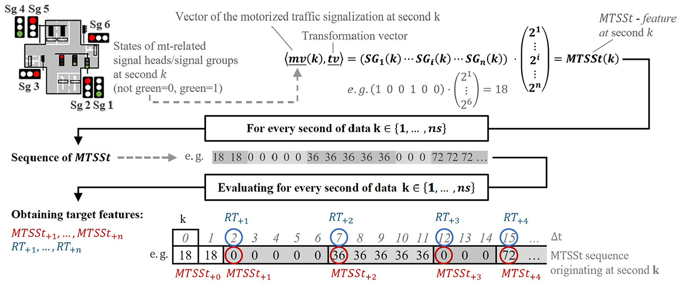
Derivation of motorized traffic signalization states (MTSSts) and target features.

The analysis of the MTSSt sequences of the intersections included in our historical data revealed that predicting 10 MTSSt-switches in advance was sufficient to consistently obtain a prediction horizon of at least 30 s. Therefore, we generated the target variables for predicting the next 10 MTSSt-switches. Models were removed for periods in which the next 10 states could not be identified because of temporal jumps within the data. These jumps were caused by SP changes, data recording failures, and the removal of certain periods during the generation of the initial data models. It should be noted that for other intersections, a different number of MTSSt-switch predictions may be required to reach a prediction horizon of at least 30 s.

Furthermore, as indicated in Figure 2, the MTSSt can also be expressed and calculated at the level of the signal head’s state. As a result, the described procedure is extendable to distinct types of applied phasing schemes, whether a NEMA scheme, a RiLSA scheme (stage- or SG-oriented signal control), or comparable schemes are applied. Based on SGs, the described calculation simply reduced the size of the calculated identifier values. However, the resulting quantity of unique switched MTSSt was the same either way. Concerning non-RiLSA phasing schemes, in cases where, for example, all MT-related signal heads in a certain phase always show green at the same time, these phases could be considered as equivalent to SGs in the described procedure.

Basic Data Models

So far, the initial data models for each second have included the current state of each signal group, each detector, the current MTSSt, the current cycle second, and, if PT is prioritized, the request states of each PT-related signal. However, STFs can be considered as time series forecasts. Particularly in the context of the circulating signalization of traffic signals, defined minimum and maximum green times, and waiting time criteria, it appears to be beneficial to incorporate information referring to the past. This is achieved by adding features that relate to the time since (TS) the last change of a state of SGs, detectors, MTSSts, and PT requests. Moreover, features are added that relate to the previous three switched MTSSts. The obtained selection of targets and features for each second, $k\in \{1,\dots ,\mathrm{length}\mathrm{of}\mathrm{the}\mathrm{data}\mathrm{frame}\}$ , that is, composing the basic data models used in the training and prediction processes of this approach, are summarized in Table 1.

Table 1.

Selection of Targets and Features Composing the Used Basic Data Models

Feature(s)	Description	Format (unit)
Targets
$\mathrm{MTSS}{t}_{+1},\dots ,\mathrm{MTSS}{t}_{+10}$	Labels of the next 10 motorized traffic signalization states (MTSSts)	Integer (-)
$R{T}_{+1},\dots ,R{T}_{+10}$	Residual times until the next 10 MTSSts are switched	Integer (s)
Basic features
$\mathrm{do}{w}_k$	Current day of the week $\mathrm{dow}\in \{1,\dots ,7\}$ (1 = Monday)	Integer (-)
$\mathrm{ms}{m}_k$	Minutes since midnight at second k	Float (min)
$t{x}_k$	Current cycle second, $\mathrm{tx}\in \{0,\dots ,\mathrm{cycle}\mathrm{length}\}$	Integer(s)
$\mathrm{MTS}{t}_k$	MTSSt at the current second, k	Integer (-)
$\mathrm{MTS}{t}_{-1},\dots ,\mathrm{MTS}{t}_{-3}$	Labels of the previous three MTSSts	Integer (-)
$\mathrm{TS}\_\mathrm{GS}{t}_{0,k}$	Time since (TS) the current MTSSt was switched	Integer (s)
$S{G}_{i,k}$	State of signal group (SG) $i\in \{1,\dots ,\mathrm{number}\mathrm{of}\mathrm{SG}\text{'}\mathrm{s}\}$ ; 1: release 0: else	Integer (-)
$\mathrm{TS}\_\mathrm{GS}\_S{G}_{i,k}$	TS last green start (GS) of each SG at second k	Integer (s)
$\mathrm{TS}\_\mathrm{GE}\_S{G}_{i,k}$	TS last green end (GE) of each SG at second k	Integer (s)
$D_{d,k}$	State of detector $d\in \{1,\dots ,\mathrm{number}\mathrm{of}\mathrm{detecors}\}$ 0: no detection, 1: detecting presence/pushed	Integer (-)
$\mathrm{TS}\_D_{d,k}$	TS detector d is detecting presence/was pushed	Integer (s)
Public transport (PT)-related features
$\mathrm{RSPTS}{G}_{u,k}$	Request state of PT-related SG $u\in \{1,\dots ,\mathrm{number}\mathrm{PTSG}\}$ 0: no registration, 1: preregistration, 2: main registration	Integer (-)
$\mathrm{TS}\_P{R}_{u,k}$	TS a preregistration was received for each PT-related SG	Integer (s)
$\mathrm{TS}\_M{R}_{u,k}$	TS a main registration was received for each PT-related SG	Integer (s)

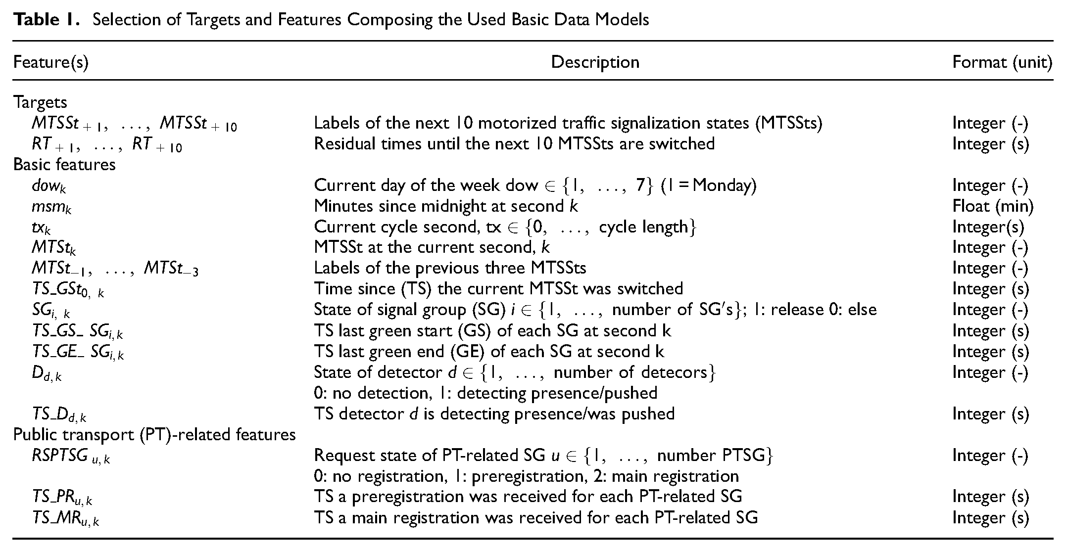
This feature selection was chosen for the ease of applicability and transferability of the STF approach to various intersections. Except for the PT features, the utilized features can be automatically generated, do not require advanced expert knowledge (e.g., for manually rebuilding every control parameter as a feature), and use only signal location plans to exclude signals that indicate danger warnings and identify MT-signals.

Even if not provided as explicit features, the scope of the given selection provides information like minimum- and maximum green times. To exemplify this: While the state of an SG is green, the TS-value will not extend beyond a specific value ( = maximum green duration), and the state of an SG will not switch from green ( = 1) to not green ( = 0) until the minimum duration expressed by a certain TS-value is reached. Suppose a coordinated release of certain SGs (traffic streams) is implemented in an SP. In that case, the given coordination for the green window(s) is derivable from the correlation between cycle second (tx) values and regularly switched green states during these periods. Certain temporal correlations can also be drawn through the msm- and the dow features. One of the main expectations of ML algorithms is that they can identify existing patterns and relationships from data, therefore, the mentioned relationships could be expected to be automatically detectable.

Prediction Procedure

This study builds on the findings of our previous approach ( 20 ) for predicting sequences of general states of signalization. It includes enhancements of the applied ML algorithm and selected features., It additionally determines the explicit STs of (MT-related) signals based on predicted MTSSt-switches. For each MTSSt-switch, two targets need to be predicted: the label of the ith next MTSSt ( $\mathrm{MTSS}{t}_{+i}$ ) and the residual time until the switch ( $R{T}_{+i}$ ). Whereas predicting the state labels is a classification task, predicting residual times is a regression task.

However, the targets of successive MTSSt-switches are related to the preceding ones: this is a crucial factor, especially for predicting switches further into the future. Certain MTSSts only have one possible successor, whereas others have multiple successors that are chosen based on the current state in the cycle and/or triggered by the traffic situation. The residual time until an MTSSt-switch depends on the durations of the preceding states, which rely on their position within the state sequence and could be influenced by traffic.

These relationships can be factored in by selecting an ML method that can learn these interdependencies and provide appropriate predictions for the targets based on a suitable selection of features extracted from current and/or past data. Additionally, a cascading prediction process can be applied, in which previous predictions are used as additional features for predicting switches further into the future. However, in the case of incorrect predictions of previous targets, these errors are also carried over and might impair the accuracy of subsequent predictions.

Selecting an ML Algorithm

Based on the results of our performance comparison (in which the application of XGBoost provided the best results [ 45 ]), on the results of a previous approach ( 50 ), and the results of additional preliminary experiments, the Python implementation of XGBoost was applied. XGBoost is a gradient-boosting framework applicable for addressing regression and classification problems ( 34 ). It uses an ensemble of decision trees to make predictions: each tree is trained to correct the errors of the previous tree and regularization is included to prevent overfitting.

For predicting the labels of the next 10 MTSSts, the XBGClassifier from the sckit-learn interface of XGBoost was used. Considering the given multiclass classification tasks, the learning objective was set to “multi:softmax.” In our earlier work, alongside XGBoost, custom-designed Bayesian networks were employed to predict the labels of the next three general states ( 50 ). Subsequently, both ML methods were combined (cascaded) to increase the accuracy of the general state predictions. However, the number of target values within the possibility space of the switched MTSSts was significantly lower than the number of switched general states. For instance, the number of switched general states of one of the considered traffic signal systems in the later described field tests was about 300, whereas only 23 different MTSSts were switched. Consequently, the computational cost for training predictive models was reduced compared with our previous study, enabling us to utilize larger amounts of training data. In addition, the average duration for which an MTSSt was switched was longer than the average switching duration of a general state, allowing coverage of the desired minimum prediction horizon of 30 s by involving fewer predicted MTSSt-switches than predicted general state switches. Because of the altered boundary conditions associated with the smaller possibility space, combined with a slightly advanced feature selection involving properly engineered PT-related features, the exclusive application of XGBoost now yielded superior results for predicting MTSSt labels.

Initially, we considered using the XGBRegressor to predict the residual times: XGBRegressor outputs continuous values. However, since a secondwise output of the residual times was desired, its predictions had to be rounded to the nearest integer second. Nevertheless, even considering all baseline regression objectives provided in the XGBboost library, the accuracy of the desired secondwise output was insufficient. During several tests, XGBClassifier outperformed XGBRegressor. Although other evaluation metrics like MAE were almost identical, XGBClassifier provided higher and sufficient accuracy for predicting residual times accurate to the second. This suggests that the necessary rounding of the continuous XGBRegressor outputs caused the observed inaccuracies. Therefore, XBGClassifier was also applied for the residual time predictions.

Sequence of Predictions

Several cascading prediction processes were pretested to further consider the relations between the targets of successive MTSSt-switches. In these pretests, several orders for predicting the 20 targets were considered, along with different selections and quantities of previously made predictions being used as additional features, extending the feature selection presented in Table 1. The tested range of previous predictions spanned from adding all previous predicted targets to including none.

We found that higher accuracies were attained by independently predicting each next MTSSt without considering the (previous) predictions of other targets. The same was found when predicting residual times until the very next MTSSt-switch, $R{T}_{+1}$ . In predictions of residual times, $R{T}_{+2},\dots ,R{T}_{+10}$ , preliminary experiments have shown that it is beneficial to use the label of the previous state ( $\mathrm{MTSS}{t}_{+n-1}$ ) and residual time as additional features until that state is switched ( $R{T}_{+n-1}$ ).

Algorithm 1: Training procedure
Input:	${\mathbf{X}}_{\mathbf{train}}$ (training samples. For each sample, ${\mathrm{X}}_{\mathrm{train}}$ includes values for each basic feature and each PT-related feature if PT is prioritized at this intersection)
	${\mathbf{Y}}_{\mathbf{train}}$ (true labels of the target features.For each sample of ${\mathrm{X}}_{\mathrm{train}},{\mathrm{Y}}_{\mathrm{train}}$ includes the true values of each target feature ${\mathrm{Y}}_{\mathrm{MTSS}{\mathrm{t}}_{+1}},\dots ,{\mathrm{Y}}_{\mathrm{R}{\mathrm{T}}_{+10}}$ )
// The training of all predictive models could also be
// executed parallelized (e. g. on different computing
// systems)
for target in [ $\mathbf{MTSS}{\mathbf{t}}_{+1},\dots ,\mathbf{MTSS}{\mathbf{t}}_{+10},\mathbf{R}{\mathbf{T}}_{+1}$ ] do
$\mathrm{XBGClassifie}{\mathrm{r}}_{\mathrm{target}}=\mathrm{XBGClassifier}.\mathrm{train}$
$(\mathrm{TrainingData}={\mathrm{X}}_{\mathrm{train}},$
$\mathrm{TrueLabels}={\mathrm{Y}}_{\mathrm{target}})$
for j = 2to10do
//Add true values to train predictive model for $\mathrm{R}{\mathrm{T}}_{+\mathrm{j}}$
${\mathrm{X}}_{\mathrm{train}\mathrm{R}{\mathrm{T}}_{+\mathrm{j}}}=\mathrm{MERGE}(X_{\mathrm{train}},Y_{\mathrm{MTSS}{t}_{+(j-1)}},Y_{R{T}_{+(j-1)}})$
$\mathrm{XBGClassifie}{\mathrm{r}}_{\mathrm{R}{\mathrm{T}}_{+\mathrm{j}}}=\mathrm{XBGClassifier}.\mathrm{train}$
$(\mathrm{TrainingData}={\mathrm{X}}_{\mathrm{train}\mathrm{R}{\mathrm{T}}_{+\mathrm{j}}},$
$\mathrm{TrueLabels}={\mathrm{Y}}_{\mathrm{R}{\mathrm{T}}_{+\mathrm{j}}})$
Output:	$\mathbf{XBGClassifie}{\mathbf{r}}_{\mathbf{MTSS}{\mathbf{t}}_{+1}},\dots ,\mathbf{XBGClassifie}{\mathbf{r}}_{\mathbf{R}{\mathbf{T}}_{+10}}$ (Trained predictive models)

Algorithm 2: Prediction procedure
Input:	${\mathbf{x}}_{\mathbf{k}}$ (input features at current second, k: basic features + [PT-related features])
	$\mathbf{XBGClassifie}{\mathbf{r}}_{\mathbf{MTSS}{\mathbf{t}}_{+1}},\dots ,\mathbf{XBGClassifie}{\mathbf{r}}_{\mathbf{R}{\mathbf{T}}_{+10}}$ (Trained predictive models)
	$\mathbf{MTSSt}\_\mathbf{Decoder}$ (MTSSt to MT signal state decoder)
// Parallelized prediction of all MTSSts
do in parallel
$\mathrm{MTSS}{\mathrm{t}}_{+1,\mathrm{k}}=\mathrm{XBGClassifie}{\mathrm{r}}_{\mathrm{MTSS}{\mathrm{t}}_{+1}}.\mathrm{predict}({\mathrm{x}}_{\mathrm{k}})$
$\mathrm{MTSS}{\mathrm{t}}_{+2,\mathrm{k}}=\mathrm{XBGClassifie}{\mathrm{r}}_{\mathrm{MTSS}{\mathrm{t}}_{+2}}.\mathrm{predict}({\mathrm{x}}_{\mathrm{k}})$
…
$\mathrm{MTSS}{\mathrm{t}}_{+10,\mathrm{k}}=\mathrm{XBGClassifie}{\mathrm{r}}_{\mathrm{MTSS}{\mathrm{t}}_{+10}}.\mathrm{predict}({\mathrm{x}}_{\mathrm{k}})$
$\mathrm{R}{\mathrm{T}}_{+1,\mathrm{k}}=\mathrm{XBGClassifie}{\mathrm{r}}_{\mathrm{R}{\mathrm{T}}_{+1}}.\mathrm{predict}({\mathrm{x}}_{\mathrm{k}})$
// Sequential prediction of the remaining RT targets
for j in [2, 3, . . . ., 10] do
//Add previous predictions according to $\mathrm{R}{\mathrm{T}}_{+\mathrm{j},\mathrm{k}}$
${\mathrm{x}}_{\mathrm{k},\mathrm{j}}=\mathrm{MERGE}({\mathrm{x}}_{\mathrm{k}},\mathrm{MTSS}{\mathrm{t}}_{+(\mathrm{j}-1),\mathrm{k}},\mathrm{R}{\mathrm{T}}_{+(\mathrm{j}-1),\mathrm{k}})$
$\mathrm{R}{\mathrm{T}}_{+\mathrm{j},\mathrm{k}}=\mathrm{XBGClassifie}{\mathrm{r}}_{\mathrm{R}{\mathrm{T}}_{+\mathrm{j}}}.\mathrm{predict}({\mathrm{x}}_{\mathrm{k},\mathrm{j}})$
// Determination of the future MT Signalization
$\mathrm{MTSi}{\mathrm{g}}_{\mathrm{k}}$  = DeterminationProcedure ( $\mathrm{MTSS}{\mathrm{t}}_{+0,\mathrm{k}},$
$\mathrm{MTSS}{\mathrm{t}}_{+1,\mathrm{k}},\dots ,\mathrm{R}{\mathrm{T}}_{+10,\mathrm{k}},\mathrm{MTSSt}\_\mathrm{Decoder}$ )
Output:	$\mathbf{MTSi}{\mathbf{g}}_{\mathbf{k}}$ (Future signalization of MT-signals for the next 30 + n seconds originating from second k)

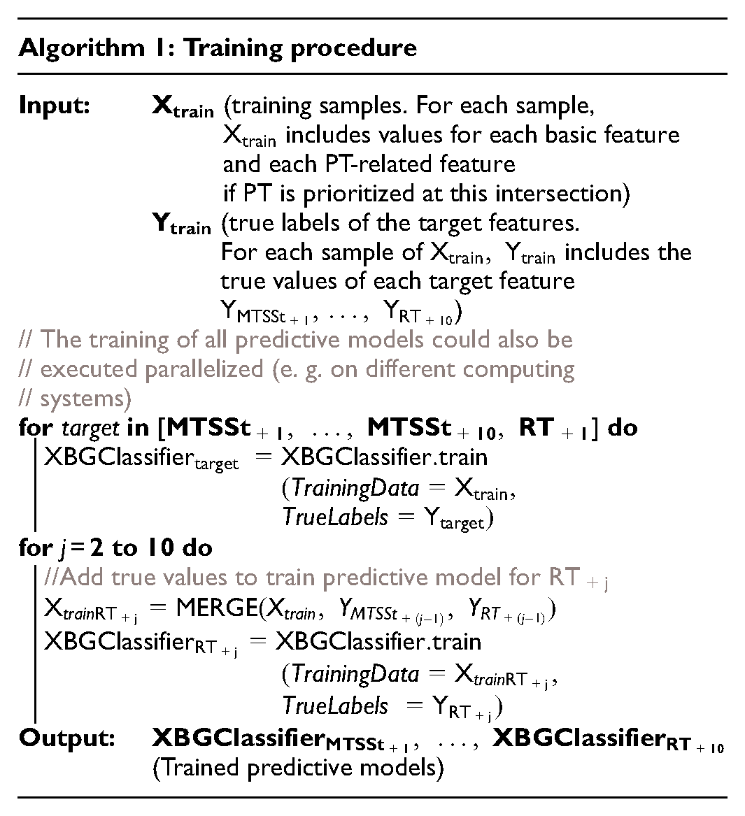
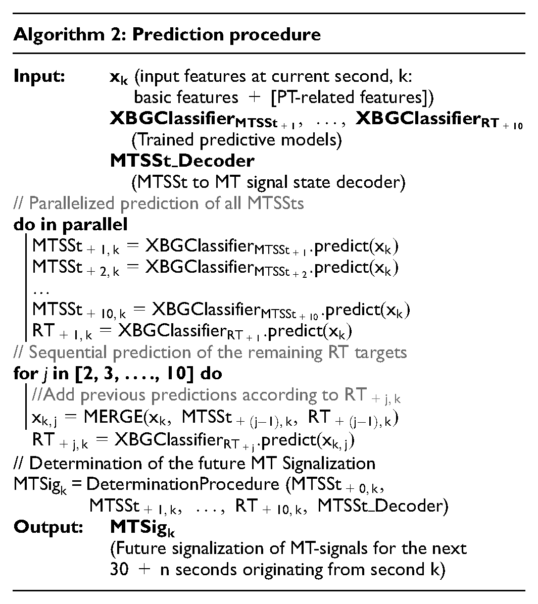
Based on these findings, the training procedure was implemented as abstracted in Algorithm 1, and the developed prediction procedure was implemented as abstracted in Algorithm 2. If previous targets are considered, their actual values are utilized as additional features to train the predictive XGBoost models. This provides an appropriate input for learning the given relationships. To visualize the differing selections of features used for training the models to predict $R{T}_{+2}$ till $R{T}_{+10}$ compared with the other targets, Algorithm 1 abstracts the training procedure in a sequential order. However, given that the true labels of the training samples are known, the predictive models could also be trained in parallel or in any order at all.

To obtain the future signalization of MT-related signals for the next 30 + n seconds, originating from the current second k, current measures of features ( $x_k$ ) were applied to the trained XGBoost models (Algorithm 2). Since the predictions of the next n states and the prediction of $R{T}_{+1}$ do not require additional features, they can be executed in parallel, enhancing the real-time applicability of the approach. The prediction of $R{T}_{+2},\dots ,R{T}_{+10}$ , however, must be carried out afterwards in a sequential order, as outlined in Algorithm 2. Subsequently, the future signalization of the MT-signals is derived by the application of a determination procedure, which is described in the following.

Determining the Future Signalization of MT-Signals

To determine the STs of individual MT-signals, a three-step derivation procedure based on the predictions of MTSSt-switches was conducted (see Figure 3).

Figure 3.

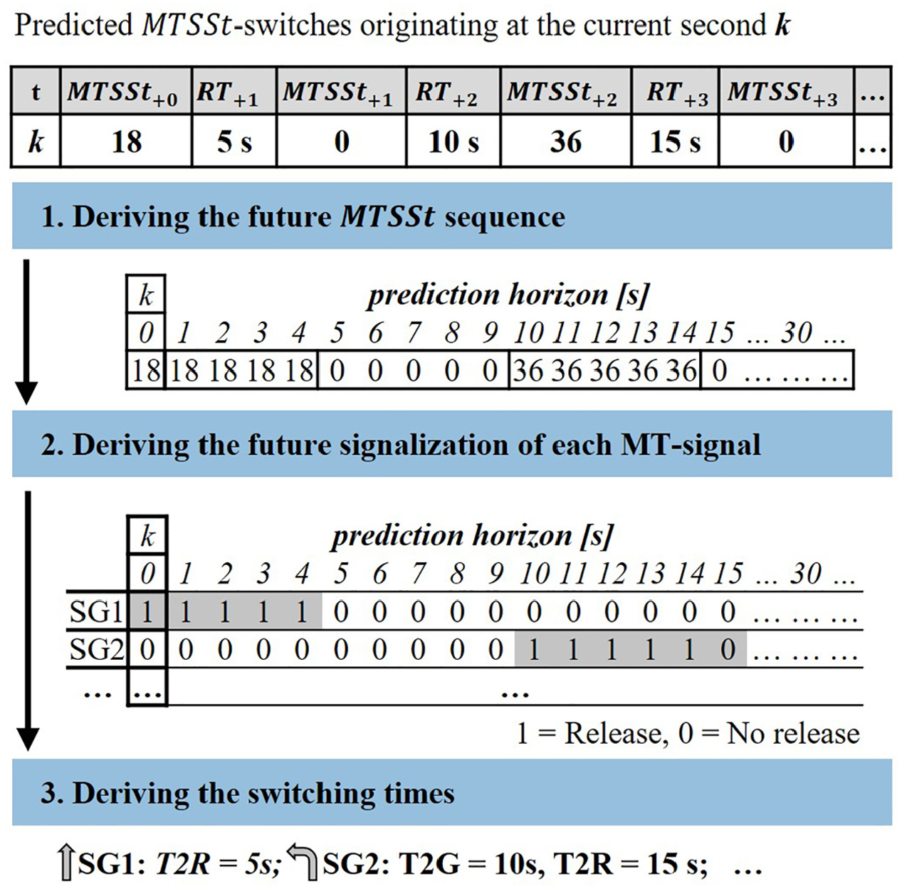
Determination of future switching times of MT-signals based on predicted MTSSt-switches.

In the first step, the future sequence of MTSSts is derived. For this, an array is gradually filled based on the predicted target values. First, the currently switched MTSSt is filled in up to the next predicted switching time. Then, the subsequent predicted states are filled according to the predicted STs. The array is filled up to the 10th MTSSt-switch. However, the filling process is stopped if there are contradictions between the residual time predictions (e.g., when a predicted $R{T}_{+j,k}$ -value exceeds a predicted $R{T}_{+(j-1),k}$ -value). Preliminary experiments have shown that the prediction accuracy decreases the further a switch is located into the future. Therefore, in case of contradictions, the size of the provided prediction horizon is left to the length of the array filled up to that point. However, within the scope of the experiments conducted in our field trial, we did not encounter a case in which an array covered less than the chosen minimum horizon of 30 s.

In the second step, the future signalization of each MT signal is derived and decoded. For this purpose, a dictionary data structure was used, in which the state of each MT signal was stored for each unique MTSSt.

The STs of the individual signals are then derived in the final step based on analyzing the sequence of their future signalization.

Field Testing

To test the accuracy of the approach, prediction experiments were conducted using historical data of three 4-way intersections and one 3-way intersection located in the city of Kassel. Each intersection was signalized by a coordinated traffic-actuated signal control with a fixed cycle time of 100 s. Each signal control took green period adjustments into account and was operated in a stage-oriented manner.

RiLSA defines a stage as “a part of a signal program during which a given signalization status remains unchanged” ( 51 ). During a stage, several nonconflicting traffic streams can have the right of way, even if they enter the intersection from different access roads. The green time of traffic streams that have the right of way during the same stage must not start simultaneously. The period of a stage extends from the green start of the last released stream until the next green end of any released stream. Conflicting traffic streams, except in certain cases for permitted right- and left-turn movements, are released in distinct stages. Transitions (periods) are switched between stages. They contain individual, predefined sequences of signaling states to ensure that conflict areas are cleared before conflicting streams are released.

The number of stages switched at each intersection differed, ranging from 6 to 20 stages (see Figure 4). At two intersections (001 and 020), the stages were run through cyclically. At the other two intersections (002 and 010), the stages were divided into multiple logic blocks, which were passed through cyclically. Whereas certain blocks contained only one stage, others contained up to four distinct stages. Which stage was switched in each block and, therefore, which movements were released depended on the current traffic situation. Not requested stages or blocks were skipped at all intersections. As a result, certain stages were switched in every cycle, whereas others, which contained, for example, PT or pedestrian releases, were only switched if requested. The number of stages or logic blocks that could be skipped differed between the intersections. At all intersections, certain traffic streams could be released more than once during a cycle.

Figure 4.

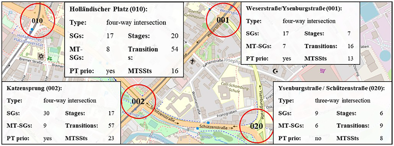
Selected intersections for field testing.

In certain cases, stages containing (almost) identical released movements were held (in several blocks). During a running cycle, this enabled the catch-up of green times for traffic streams that were not previously requested or were skipped owing to the switching of a prioritized stage. Furthermore, deviations from the predefined characteristics of the signal state pattern of transition periods described in the RiLSA ( 51 ) were possible at the given intersections. Given the traffic-actuated control operation, referred to as transition manipulation, if certain conditions were satisfied, a running transition could be aborted in favor of a transition to another stage before the overall state of the stage was reached. PT was prioritized at three of the four intersections, which allowed coordination to be abandoned in favor of PT releases. These three intersections (001, 002, and 010) were passed by public buses and streetcars. Depending on the route, the buses used both the roadway and the streetcar lanes, meaning them also requested releases of MT-signals.

Four different traffic-actuated SPs were applied at each intersection. Each SP was tuned for specific traffic-demand scenarios and the given intersection:

• SP1: morning (peak) hours (5:30 to 8:30 a.m.),

• SP2: daytime outside of peak hours (8:30 a.m. to 2:30 p.m., 6:30 to 9:00 p.m.),

• SP3: afternoon (peak) hours (2:30 to 6:30 p.m.),

• SP4: late evening and night hours (9:00 p.m. to 5:30 a.m.).

Train and Test Data Splits

Data models generated on raw data logged between February and April 2023 were used for conducting the prediction experiments. To evaluate the approach, specifically the ability of the predictive XGBoost models, to generalize to new unseen data, the selected data models are split into several training and test data splits.

To consider differing traffic loads and demand scenarios, ranging from peak traffic volumes during peak hours to (very) low traffic volumes during the late evening and early morning hours, data models based on data during the active times of SP2, SP3, and SP4 were selected.

The SPs applied at each intersection were individual solutions tuned according to the specific traffic demands, the number of SGs, the allowed movement combinations, the number and location of installed detectors, the degree of traffic adaptivity, and the given geometries at the particular intersection. This necessitated training predictive models for each intersection individually. Furthermore, programs SP2, SP3, and SP4 applied at the same intersection differed with regard to varying minimum and maximum green durations or allowed orders of stage switches. For example, deviating from the previous general descriptions, a coordinated main direction steady green circuit was applied during the runtime of SP4 at Intersection 001. Stage switches were only conducted in those terms if competing traffic streams requested them. As a result, we trained individual models for each of the considered SPs.

As shown in Figure 5, for SP2 and SP4 of each intersection, 400,000 samples (~ 111 h of data) from the data model of the previous month were picked randomly as training data, and the first 400,000 samples from the following month were selected as test data. This means that data from February were used to train predictive models, which were then used to make predictions on the data from March. Conversely, the data from March were used to make predictions for April. The continuous test samples were selected to evaluate the generalizability of the predictive models under realistic conditions in which continuous predictions were required. Nevertheless, certain time jumps were systematically present in the data when the running SP changed or if, as outlined in the data preparation subsection, the data logging failed or was incomplete. Comparatively high numbers of test samples were selected to cover the scope of different daily and weekly demand scenarios during the active runtime of the specific SP.

Figure 5.

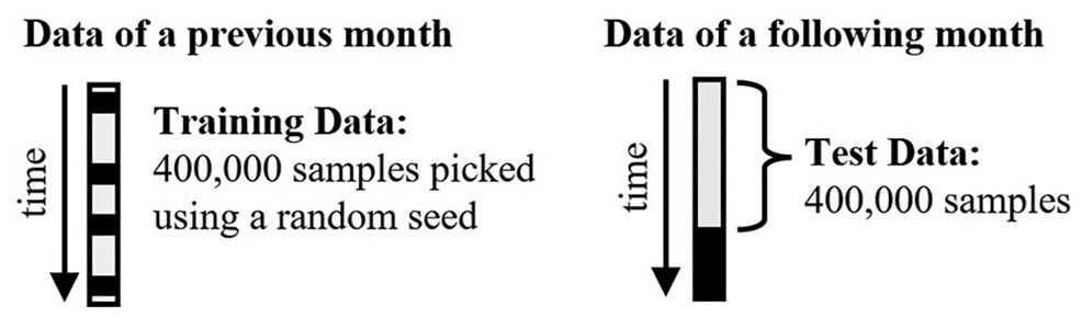
Illustration of the applied train/test splits for data models of SPs 2 and 4.

The same monthly splits were conducted for the data models consisting of data logged during SP3’s runtime, except that a lower number of samples was used for each of the train/test splits. This was because of SP3’s respective lower monthly runtime. With 150,000 selected samples for the training and test data splits, a comparable share as for SP2/SP4 was applied.

A training procedure, as outlined in Algorithm 1, was applied to train the predictive models, and the same selection of slightly adapted standard hyperparameters was used. A grid search was conducted before the primary experiments of the field study to tune the hyperparameters. Because of the scope of the study for the intersections and target variables considered, the scope of hyperparameter optimization was limited to using the data only from Intersection 002 of November 2022 for this task. However, it should be noted that further individual adjustments of the hyperparameters for training the predictive models for predicting each of the 20 target variables of each intersection could lead to (slightly) better results.

The trained predictive models and the corresponding test data were then applied to the developed prediction procedure (Algorithm 2). For each test sample, this provided a predicted complete second-by-second signalization sequence for each MT signal, which was compared with the ground truth.

Thereby, using our computing resources, predicting the future signalization sequence of each MT-related signal for one test sample was completed in less than 10 ms in total. Following the prediction procedure outlined in Algorithm 1, the required time was distributed as follows: approximately 0.4 up to 0.9 ms for predicting the first 11 target variables in parallel, about 6.5 ms for the subsequent sequential predictions of the remaining target variables, and approximately 1.4 ms for applying the determination procedure.

Statistical Baseline Method (BLM)

To evaluate whether the effort required to apply the proposed ML approach was worthwhile, additional predictions were made for the test data using a statistical-based prediction approach, which served as a baseline.

Inspired by the studies of Protschky et al. ( 37 ) and Mathew et al. ( 53 ), for this reference method, the training data sets were used to calculate probabilistic green distributions for each MT-related signal. These distributions included the probability of green for each second in the cycle, as exemplified in Figure 6. To estimate the future states of each signal for the next 30 s, the following procedure was applied:

Figure 6.

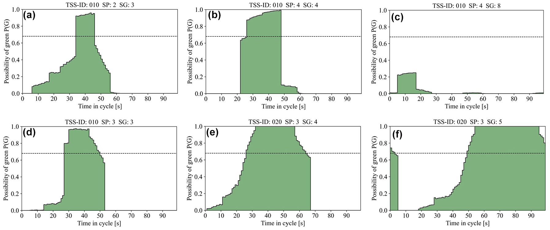
Exemplary green possibility distributions: (a) TSS 010 SP2 SG3, (b) TSS 010 SP4 SG4, (c) TSS 010 SP2 SG8, (d) TSS 010 SP3 SG3, (e) TSS 020 SP3 SG4, and (f) TSS 020 SP3 SG5.

First oriented by the current second in the cycle, the future signalization sequence was filled with the probability of green for the next 30 s using the green distributions. In the next step, (following Protschky et al.’s methodology [ 37 ]), a confidence threshold was applied (illustrated by the dotted lines in Figure 6). For all possible values above the threshold, the future signal state for this cycle second was assumed to be green or, vice versa, not green if the possibility for green was below the threshold.

For tuning the baseline method (BLM), we considered and tested the confidence probability values for SAE J2735 messages proposed by the V2X Core Technical Committee ( 54 ) to find suitable threshold values. Furthermore, distributions storing the possibility of green during specific periods (e.g., 10:00 to 11:00 a.m.) were considered. On average, the best results concerning the performance metrics were achieved by applying a threshold of 56%, which refers to an SAE J2735 confidence value of 3. Furthermore, we found that using multiple distributions, which stored the possibility of green for specific periods of the SP’s active time, enhanced the performance of the BLM.

Given its statistical characteristics, the BLM can provide relatively decent estimates if the green distribution resembles a pretimed shape, as shown in Figure 6, b and d . In contrast, less decent estimates can be expected if the green distributions are shaped like Figure 6a. Further, it was evident that this method would fail to provide reliable estimates for SCs if certain phases were not switched in every cycle (Figure 6c). In such cases, the BLM assumes that the signal is always red, as the threshold is never reached.

Results and Discussion

The approach was evaluated for the chosen minimal provided prediction horizon of 30 s, which was covered by the predicted sequence of each test sample, using the evaluation metrics described below.

This prediction approach’s (total) accuracy (ACC, Equation 1) is considered as the share of signalization sequences of MT-signals that are predicted accurately to the second, without any deviation, for the evaluation horizon of 30 s. As red times are often longer than 30 s, especially when certain releases must be requested, not every signalization sequence includes a release, specifically, an SC. Conversely, some sequences only contain releases when green times are longer than 30 s. Therefore, a further distinction can be made between sequences that contain at least one SC (switch sequences) and sequences that do not contain any SCs.

Following this distinction, in Equation 1, switch sequences that are correctly predicted are denoted as true positives (TPs), whereas incorrectly predicted switch sequences are represented as false positives (FPs). The same nomenclature applies to nonswitch sequences. Correctly predicted nonswitch sequences are referred to as true negatives (TN), and incorrect ones are referred to as false negatives (FNs).

$$\mathrm{ACC}=\frac{\mathrm{TP}+\mathrm{TN}}{\mathrm{TP}+\mathrm{TN}+\mathrm{FP}+\mathrm{FN}}$$

(1)

In the context of GLOSA applications, the correct SC from red to green and vice versa must be predicted ideally with only minor deviations. Therefore, the following additional evaluation metrics were used.

The measure of precision (positive predictive values [PPV], Equation 2) indicates how many of the predicted SCs match the ground truth. The sensitivity (true positive rate [TPR], Equation 3) is the ratio of correctly predicted SCs to all actual SCs of the ground truth. Thereby for both measures, whether the correct SCs are contained in the predicted signalization sequence is checked. Therefore, in Equations 2 and 3, correctly predicted SCs are denoted as TPs), whereas incorrectly predicted SCs are referred to as FPs. SCs that are present but are not predicted are termed FNs.

$$\mathrm{PPV}=\frac{\mathrm{TP}}{\mathrm{TP}+\mathrm{FP}}$$

(2)

$$\mathrm{TPR}=\frac{\mathrm{TP}}{\mathrm{TP}+\mathrm{FN}}$$

(3)

$$\mathrm{MAE}=\frac{1}{n}\sum _{i=1}^n(|{\hat{y}}_i-y_i|)$$

(4)

To measure the prediction error (deviation) for accurate SC predictions, MAE (Equation 4) was applied, where ${\hat{y}}_i$ denotes the predicted value of the time until an SC i, and $y_i$ represents the actual time until value of the ground truth.

An accurate prediction approach achieves high values for precision and sensitivity and a low MAE. This means that most SCs are predicted with only minor deviations, and only a few false predictions are made.

Daytime Periods Outside of Peak Hours

Table 2 summarizes the results of predictions made for periods outside of peak hours during the daytime.

Table 2.

Obtained Results for Predicting the Future Signalization for Nonpeak Daytime Hours

TSS	Matching signal state sequences				Signal changes		Temporal deviation of SC predictions
	Ratio	ACC			PPV, %	TPR, %	MAE, s
	SwSq	SwSq, %	non-SwSq, %	Ø, %			0–10 s	11–20 s	21–30 s	0–30 s
001	0.53	66.9	96.6	81.0	95.6	95.9	0.50	1.34	1.36	1.05
002	0.45	65.0	96.9	82.4	94.4	94.7	0.42	1.18	1.31	0.95
010	0.46	62.2	97.2	81.2	95.2	95.5	0.60	1.50	1.47	1.18
020	0.48	69.5	98.0	84.1	97.0	96.3	0.64	1.38	1.11	1.04
Ø	0.48	65.6	97.1	82.1	95.4	95.5	0.52	1.34	1.33	1.06
BLM		26.8	90.3	59.9	76.6	88	3.21	3.62	3.15	3.29
ΔØ-BLM		+38.80	+6.8	+22.2	+18.8	+7.50	−2.69	−2.28	−1.82	−2.23

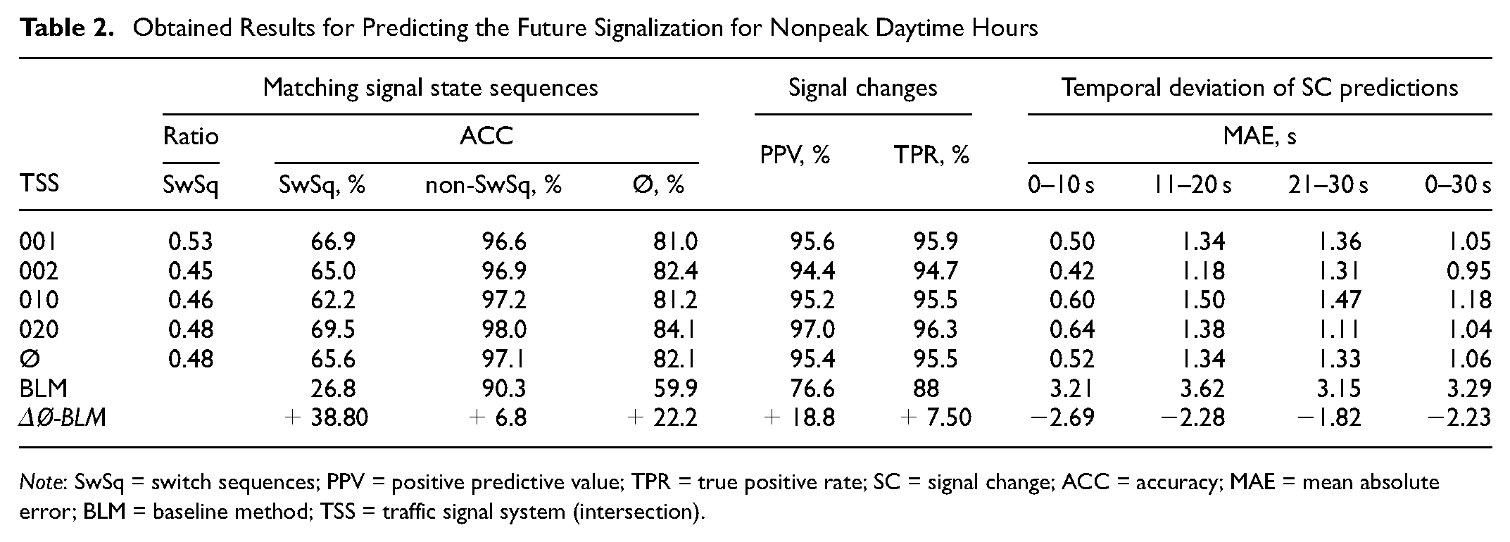
Note: SwSq = switch sequences; PPV = positive predictive value; TPR = true positive rate; SC = signal change; ACC = accuracy; MAE = mean absolute error; BLM = baseline method; TSS = traffic signal system (intersection).

Signalization Sequences

In 82.1% of all cases, the future signalization sequence of MT-signals during the next 30 s was predicted accurately to the second, without any deviation (Table 2). In 17.9% of all cases, predicted sequences deviated from the ground truth for at least 1 s. Approximately two-thirds of all predicted switch sequences (SwSq) matched the ground truth. However, most sequences that were not predicted accurately to the second contained at least one SC. On the other hand, most of the nonswitch sequences (non-SwSq) were predicted entirely correctly. Only about 3% did not match the ground truth. Thus, in 97% of the cases, when a signal maintained its state (green/red), the predictions made were accurate. With regard to the results of each intersection, accuracy was in the same range for all intersections. However, the results for Intersections 001 and 010 were slightly worse than those of the other two intersections. The ML approach outperformed the BLM. Thereby, signalization sequences that contained at least one SC were predicted with more than twice the confidence of applying the reference method.

Signal Changes and Switching Times

The determined predicted signalization sequences contained up to three SCs. Measured over all the intersections, the SCs were predicted at a high precision of 95.4% (Table 2). That means 954 of 1,000 predicted SCs occurred in the ground truth. Furthermore, a high overall sensitivity value of 95.5% was achieved, which means that, on average, only 45 out of 1,000 SCs in the ground truth were not predicted. For the results for each intersection, the best PPV and TPR values were obtained for the SC predictions at Intersection 020. The MAE values for the time until an accurately predicted SC occurred, averaged over the entire evaluation horizon, ranged between 0.95 s for Intersection 002 and 1.2 s for Intersection 010 (Table 2).

As can be deduced from the higher share of accurately predicted switch sequences, compared with the BLM, the XGBoost models provided more accurate predictions of SCs and residual times until their switchover. The, for the BLM observable, only slightly different MAE values for varying prediction horizons (Table 2) are due to the statistical calculation nature of the BLM.

In contrast, as shown in Table 2 and further visualized in Figure 7, the mean absolute deviation of switch times, predicted by the ML approach, decreased with decreasing prediction horizons. The slightly decreasing trend of MAEs for horizons beyond 20 s was because of the limitation of the evaluation period to 30 s, which systematically restricted an overestimation of the time until an SC. Although the lowest precision and sensitivity values were achieved for Intersection 002, its T2SC predictions showed the lowest temporal deviation overall and for horizons smaller than 20 s (Table 2 and Figure 7). Assessed over the entire evaluation period, the mean deviation of predicted switch times was highest for Intersection 010, showing a maximum deviation of about 1.7 s for a prediction horizon of 20 s.

Figure 7.

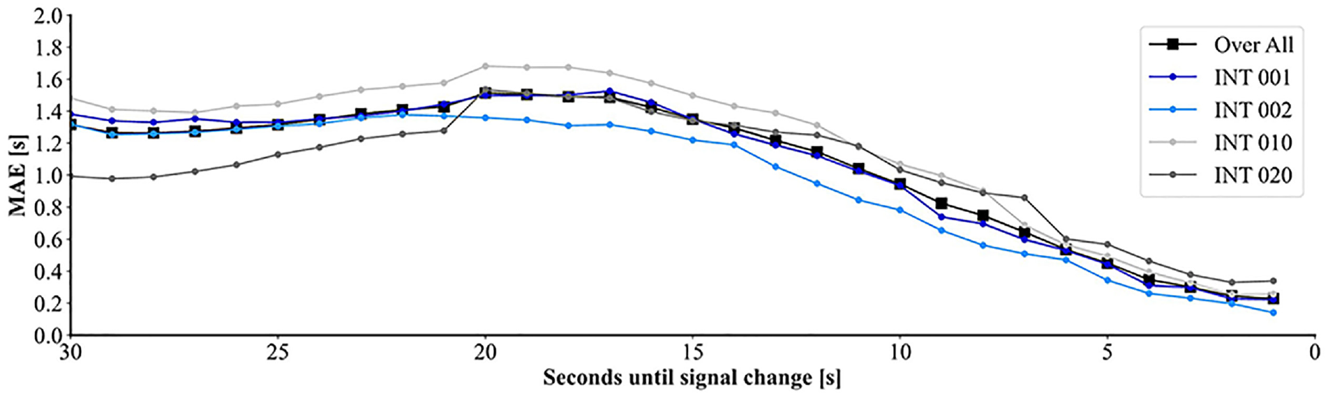
Mean absolute error in relation to the time until a signal change.

Figure 8 shows the absolute error distribution across all intersections, and by applying the ML approach all approximately 13 million accurately predicted SC from red to green and vice versa. The outliers are the points at larger distances than the 1.5 times interquartile range from the mean error values. The very small interquartile ranges indicated that most predicted STs deviated only slightly from the actual change times. Especially for prediction horizons below 10 s, most T2SC predictions had almost no deviation. Nonetheless, small interquartile ranges contributed to the outliers. As observed, these outliers ranged up to the maximum possible deviation inside the evaluation horizon. However, a proportion of the strongest outliers, in particular, can be traced back to slightly different predicted MTSSts, specifically deviating MTSSt sequences. MTSSt labels indicated the signal status combination of the MT-signals. Therefore, if a deviating combination is predicted, that could only differ in the status of one single signal, this could contribute to outliers.

Figure 8.

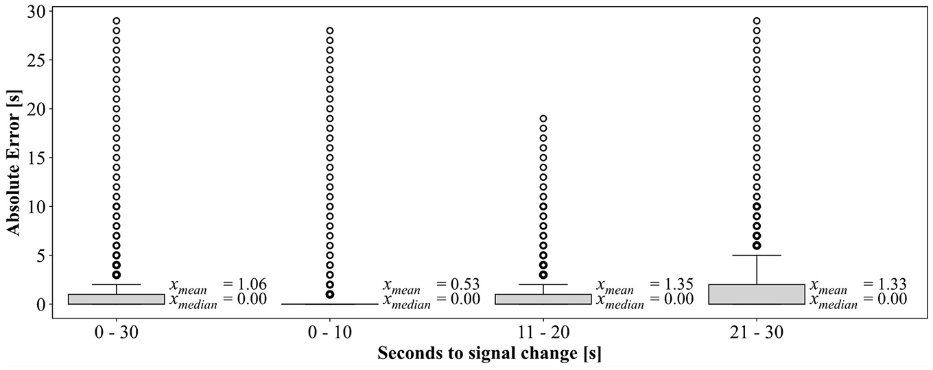
Average absolute error distributions of predicted switching times.

In summary, the differences overall in the results obtained for the individual intersections were small. The findings suggest that, for periods of daily traffic loads outside of peak hours, the application of the proposed framework could provide reliable estimates of the future signalization of MT-signals at various traffic-actuated signalized intersections. However, as expected, slightly better results were achieved for the three-way intersection, 020, because PT was not prioritized at this intersection, and its signal control was the least complex in the scope of the selected intersections. Conversely, slightly worse results were obtained for Intersection 010, the most heavily frequented intersection by pedestrians and PT, located between the University of Kassel campus and the city center, explaining the slightly lower performance compared with other intersections.

Late Evening till Early Morning Periods

Comparably (very) low traffic volumes were present at the given intersections during late evening and early morning hours. In those periods, arrivals and green-time requests had a comparatively higher stochastic nature. Owing to the likely lack of further (competing) green-time requests, a comparatively higher responsiveness of the control system to these requests can be expected. These conditions initially indicated that providing accurate predictions of STs would be more challenging during those periods. However, it was the opposite case for periods with almost no or only very sporadic traffic during the night hours. In those periods, at Intersections 002, 010, and 020, because of lacking requests from competing traffic streams, in most cycles, only the coordinated stages in the main and secondary directions were switched alternately. This represents a comparatively easily predictable switching pattern. In consideration of the described circumstances, the predictions were evaluated separately for two distinct periods:

• a) Nighttime hours between midnight and 4.30 a.m., and

• b) Periods between 8:00 or 9:00 p.m. until midnight and from 4:30 to 5:30 a.m.

The results obtained for predictions made during the operation period of SP4 are summarized in Table 3.

Table 3.

Obtained Results For Late Evening, Early Morning, And Night Hour Periods

TSS	Matching signal state sequences						Temporal deviation of SC predictions
	Ratio	ACC			Signal changes		MAE, s
	SwSq	SwSq, %	non-SwSq, %	Ø, %	PPV, %	TPR, %	0–10 s	11–20 s	21–30 s	0–30 s
a)
001	0.44	58.3	95.6	79.3	93.3	92.3	0.58	1.05	1.30	0.97
002	0.37	81.2	99.0	92.4	97.7	93.7	0.29	0.55	0.57	0.47
010	0.44	94.8	99.5	97.4	99.1	99.1	0.08	0.18	0.18	0.15
020	0.40	93.8	99.7	97.3	99.4	98.6	0.07	0.14	0.15	0.12
Ø	0.41	84.1	98.7	92.7	97.6	96.3	0.23	0.43	0.48	0.38
BLM		47.7	91.6	73.6	74.6	80.9	2.15	2.52	2.14	2.28
ΔØ-BLM		+36.4	+7.1	+19.1	+23.0	+15.4	−1.92	−2.09	−1.66	−1.90
b)
001	0.55	56.4	94.3	73.3	94.1	94.1	0.67	1.41	1.52	1.18
002	0.43	62.4	96.4	81.6	93.7	93.5	0.47	1.12	1.48	1.00
010	0.45	82.0	98.0	90.9	96.7	97.9	0.29	0.64	0.78	0.57
020	0.48	77.7	98.3	88.7	97.4	95.8	0.32	0.63	0.72	0.55
Ø	0.48	67.3	96.6	82.7	95.1	95.1	0.47	1.03	1.20	0.89
BLM		27.2	90.5	60.3	76.0	81.9	2.44	3.47	3.30	3.03
ΔØ-BLM		+40.1	+6.1	+22.4	+19.1	+13.2	−1.97	−2.44	−2.15	−2.14

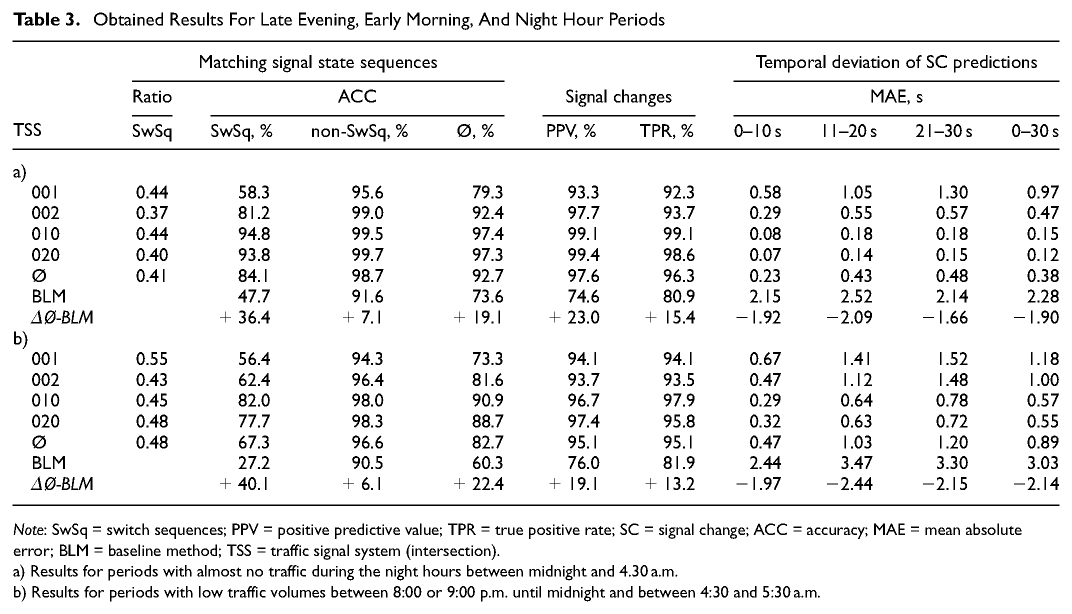
Note: SwSq = switch sequences; PPV = positive predictive value; TPR = true positive rate; SC = signal change; ACC = accuracy; MAE = mean absolute error; BLM = baseline method; TSS = traffic signal system (intersection).

a) Results for periods with almost no traffic during the night hours between midnight and 4.30 a.m.

b) Results for periods with low traffic volumes between 8:00 or 9:00 p.m. until midnight and between 4:30 and 5:30 a.m.

Signalization Sequences

Overall, signalization sequence predictions made for periods during the night hours between midnight and 4.30 a.m. were accurate to the second in 92.7% of all cases (Table 3). The statistical reference method provided a visibly smaller share of accurately predicted sequences. For Intersections 010 and 020, with accuracies above 97%, near-perfect estimates were obtained by applying the proposed ML approach. This could be interpreted as an indicator of an almost pretimed switching behavior. Nevertheless, compared with the ML approach, the BLM achieved 10%, respectively 15% lower share of deviation-free predictions of the signalization sequences for those intersections. The shares of deviation-free predicted signalization sequences obtained for low traffic volume periods (i.e., [b] in Table 3), were about 6% to 12% lower than those for the night hours. Nevertheless, the average achieved accuracy values were in the same margin as the prediction accuracies for daytime periods outside of peak hours (Tables 2 and 3). This was also true of the performance benefit of the applied XGBoost models compared with the BLM.

Signal Changes and Switching Times

The same tendencies as observed for the quality for predicting the signalization sequences was observed for the obtained PPV, TPR, and MAE values of the determined SCs. For the night hours, (i.e., [a] in Table 3), SCs were predicted with near-perfect PPV and TPR values, and only minor temporal deviations of the residual times determined from the ground truth (Table 3). For the low traffic volume periods, (b), the obtained prediction quality was slightly lower but had an overall range in the same margin as the predictions made for periods during the daytime outside of peak hours (Tables 2 and 3).

Overall, the obtained results suggest that application of the proposed framework can provide reliable estimates of the future signalization of MT-signals for low traffic volume periods.

However, in contrast to the predictions made for periods during the day outside of peak hours, distinct differences in the individual quality of the predictions made for the different intersections were found. The highest quality was obtained for Intersection 010. This can be attributed to the disruptive influences of pedestrians and a high PT frequency on the prediction quality, which were prevalent during the day given the proximity to the university, but were not present during the runtime of SP4. In the evening and at night, compared with intersection 010, Intersection 002 was traveled more frequently in all directions owing to its bottleneck location being a connecting element, resulting in more frequent releases of uncoordinated turning movements—this may explain the lower prediction quality shown here. Additionally, the SP of Intersection 002 provided higher temporal flexibility because of a higher number of skippable stages (logic blocks).

In comparison, the results for Intersection 001 were the worst, which was expected owing to the applied coordinated main direction steady green circuit at Intersection 001 during the runtime of SP4. The steady stage can remain switched for multiple cycles if no green-time request for competing traffic streams occurs. This increases the difficulty in accurately predicting the residual green times of coordinated signals, with a greater lead time to the switchover point, as the only reliable indication of an upcoming SC is derived from a detected green-time request of a competing traffic stream.

Afternoon (Peak) Hour Periods

Table 4 summarizes the obtained results for predictions made for the afternoon (peak hours).

Table 4.

Obtained Results For Predicting The Future Signalization For Afternoon (Peak) Hour Periods

TSS	Matching signal state sequences						Temporal deviation of SC predictions
	Ratio	ACC			Signal changes		MAE, s
	SwSq	SwSq, %	non-SwSq, %	Ø, %	PPV, %	TPR, %	0–10 s	11–20 s	21–30 s	0–30 s
001	0.53	81.4	98.7	89.5	98.7	96.5	0.43	1.00	0.55	0.67
002	0.47	84.4	92.1	92.1	98.0	96.9	0.31	0.57	0.52	0.47
010	0.46	68.3	98.3	84.3	97.0	95.8	0.66	1.20	0.52	0.95
020	0.52	60.9	97.4	78.6	96.5	93.3	1.11	2.10	1.26	1.51
Ø	0.49	74.8	98.3	86.7	97.6	95.7	0.59	1.14	0.79	0.84
BLM		60.2	93.6	77.1	88.3	94.8	1.8	1.90	1.19	1.65
∆ Ø-BLM		+14.6	+4.7	+9.6	+9.6	+0.9	−1.21	−0.76	−0.41	−0.81

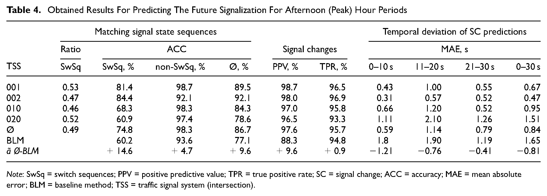
Note: SwSq = switch sequences; PPV = positive predictive value; TPR = true positive rate; SC = signal change; ACC = accuracy; MAE = mean absolute error; BLM = baseline method; TSS = traffic signal system (intersection).

Signalization Sequences

Measured over all the intersections, in 86.7% of all cases, the future signalization sequence was predicted accurately to the second. Approximately three-quarters of all predicted switch sequences matched the ground truth, and more than 98% of the nonswitch sequences were predicted correctly.

Overall, the accuracy for the afternoon hours was higher than for non-peak hour periods during the daytime, early mornings, and late evenings (Tables 2 to 4).

Signal Changes and Switching Times

The same tendency of higher accuracies can be observed for the determined SC predictions and the temporal deviations of the SC predictions. On average, 976 of 1,000 predicted SCs occurred in the ground truth, and only 43 out of 1,000 SCs occurring in the ground truth were not predicted.

Relating to the overall higher qualities of the predictions, a common assumption is that, during peak traffic hours, traffic-actuated signal controls’ switching behavior often converges to the switching behavior of pretimed signal controls. Because of the higher traffic density and volume, especially if intersections are constantly congested, certain detectors will be actuated, almost continuously with only short interruptions during green periods, indicating constant release requests. Therefore, it is likely that the same pattern of signalization will be switched cycle for cycle until the input situation (i.e., demand for releases) changes. In particular, if high numbers of stages (phases) are switched continuously, the traffic-actuated, time-related variability of green times decreases.

Compared with its performance for lower traffic volumes, performance of the BLM for peak traffic periods was noticeably better (Tables 2 to 4). Further, smaller performance disadvantages compared with the ML approach were present. This indicated that during peak periods, a converging to pretimed switching behavior can be assumed for three of the intersections under consideration. However, whereas the results of the ML-based approach obtained for Intersection 020 still promised reliable predictions, they were slightly worse than those obtained for periods with lower traffic volumes. As shown in Figure 6, e and f, based on the displayed green possibility distributions, the signalization of this junction did not converge to a pretime pattern at higher traffic loads. The three-armed intersection geometry resulted in fewer turning relationships and, consequently, fewer green splits. In particular, the through signals had green permit windows with a large span. Therefore, a stronger temporal variability in green probabilities was present, resulting in higher fulfillment rates of time gaps or congestion conditions combined with the long green permission ranges.

As the example of Intersection 020 illustrates, during peak traffic hours, an against-pretime-converging switching behavior associated with higher STF qualities should not be expected to be universally valid.

Conclusions and Future Works

Cooperative applications, such as GLOSA and RLVW systems, require a constant input of reliable estimates of the future signalization of traffic signal systems. This paper presents a framework for predicting the future signalization of traffic-actuated signals. A three-step methodology consisting of data preparation, tuning the prediction procedure, and testing the prediction approach has been described. The approach was tuned to continuously provide estimates of the signalization of MT-related signals for at least 30 s in advance. The methodology was applied and evaluated on the data of four traffic-actuated signalized intersections.

The proposed ML approach outperformed a statistical-based reference method in every scenario. For periods during the daytime outside of peak hours, the results of the field study showed that in 82% of all cases, the whole sequence of switched signals within the next 30 s was predicted accurately, without any deviations. If a signal remained in its state (green/red) for at least the next 30 s, this was estimated at an accuracy of 97%. Within this period, SCs were predicted with an average precision and sensitivity of around 95.5% with, on average, only minor temporal deviations. Only minor differences were found between the results obtained for the different intersections. A similar prediction quality was achieved for periods with low traffic volumes during late evening and early morning hours. Overall, higher accuracies were obtained for peak traffic periods. Nevertheless, distinct differences in the individual quality of the predictions made for the different intersections were observed, which can be traced back to the differing complexity of the applied SPs and traffic loads within those periods.

Overall, it can be concluded that the presented approach promises reliable estimates of the near future signalization and switching times of traffic-actuated signals during, for an application of GLOSA, suitable large a period of the next 30 s.

Since the approach only considered a given interdependency between signals, it is theoretically applicable at any signalized intersection, regardless of the type of applied phasing scheme. The selection of features used in this publication was chosen to facilitate applicability and transferability. Except for the PT features, the features implemented in our approach can be generated automatically, without advanced expert knowledge, by using only signal location plans to exclude signals that indicate danger warnings and to identify MT-signals.

The chosen ML method, XGBoost, in combination with the provided feature selection and prediction procedure, provided well-generalized models on large amounts of unseen data. This is advantageous for potential live applications, as it indicates that it may not be necessary to retrain predictive models frequently within shorter intervals to obtain reliable estimates. Nevertheless, training new models with current or representative data should be considered if decreasing (long-term) trends in the prediction accuracy can be determined. In the scope of a live application, the accuracy could be determined by comparing predictions with actual switches. In this context, the required temporal and computational effort for training new XGBoost models did not appear to be a critical factor. XGBoost is designed to deal efficiently with large data sets and is generally known to require comparatively short training times, even for complex models. Based on our experience, given sufficient computing power, and following the proposed parallelized training procedure, we assume that a training cycle for new models could be conducted within a few hours to a day, depending on the number of involved features and training samples.

However, it is essential to emphasize that there were no latencies in data transmission within the testing process using historical data, as might occur in a real-time application. Nevertheless, the presented approach is extendable from its reliance on historical data. In a real-time application, the features used to train the predictive XGBoost models could be obtained by live logging the states of signals and detectors and PT announcement messages to make predictions.

Despite the promising performance of the proposed approach, given the chosen feature selection, the systematic inclusion of expert knowledge could improve the approach’s accuracy further, for example, by including features that relate to those used by signal control units: features that track whether certain conditions like minimal green time, waiting time, or time gap criteria are satisfied. For engineering such features, input data of the logged status changes of detectors could be processed specifically according to the defined purposes of the respective detectors. Further, removing redundant features could enable the ML algorithm to better identify the given relationships. In this context, it could be beneficial to express information from multiple detectors with the same function, e.g. measuring the temporal gap between vehicles, that are installed in several lanes of the same traffic flow(s) in one feature. This could also be done for information on the scope of pedestrian push buttons that detect green-time requests for the same crossing.

Furthermore, an ensemble of predictive models could improve the prediction accuracy. Such an ensemble could consist of models based on several different ML algorithms. On the other hand, alongside a generalized model, multiple specialized models could be utilized that are trained on specific subselections of features/data to be used situationally if specific traffic or actuation situations occur. For example, if the traffic demands at an intersection change significantly for a limited period associated with major events, providing a specialized model for those periods could be beneficial.

In future works, we want to address the described potential. We would additionally like to apply the proposed framework to the data of traffic signals controlled by a non-RiLSA phasing schemes (e.g., a NEMA phasing scheme) to prove its theoretical transferability. Furthermore, based on the promising results, we are considering testing the approach in a real-time scenario. Furthermore, by increasing the number of MTSSt-switch predictions to cover a constantly larger minimal prediction horizon, the approach could be evaluated for whether it can provide suitable input for routing applications.

An essential factor for providing accuracy in larger prediction horizons and improving the accuracy, especially during low traffic periods, with highly stochastic arrivals of vehicles, could emerge from the anticipation of future detector actuation scenarios. To achieve this, upstream-located detectors could be utilized, as proposed by Mousa et al. ( 42 ). However, instead of specially installing additional detectors, an investment-free option could be considered, that utilizes detectable information at neighboring intersections. Valuable information might include the detection of vehicles at an upstream intersection, which could help to determine vehicles approaching the downstream intersection. This information, combined with the specific distance between upstream and downstream intersections and with known current and past signalizations of the upstream intersection, could facilitate forecasting the arrival (times) of vehicles at downstream intersections.