
Abstract
Traffic forecasting can enhance the efficiency of traffic control strategies such as routing decisions, variable speed limits, and ramp metering, resulting in a decrease in congestion, pollutants, and expenses, and an improvement in journey time predictability. Traffic forecasting, however, remains challenging because of the complex, heterogeneous, and cyclic nature of traffic data. To address this complexity, this research employs a multi-input hybrid deep self-attention network (MIHDSAN) for multilocation forecasting. The model inputs are selected using correlation analysis. New tunable loss and evaluation metrics formulations are proposed based on the traffic-modeling Geoffrey E. Havers (GEH) statistic. The proposed method was validated on two independent real-world traffic datasets from Stockton and Oakland, California. The weekly periodicity was the more relevant periodic input feature compared with daily variations; however, the daily variation was also significant for the Stockton dataset. The inclusion of weekly traffic periodicity (>95% correlated) improved the performance of the model by 3%. Adding daily periodicity was only beneficial for the Stockton dataset (91% correlated). The proposed GEH metric and its standard acceptance criterion offer both quantitative and qualitative means of evaluating the forecasts produced. The GEH loss function was consistent and outperformed current industry-standard methodologies of mean absolute error (MAE) in 80% and mean squared error (MSE) in 94% of cases. Therefore, this research presents evidence to suggest that the proposed GEH loss and evaluation functions validated in this paper become a standard criterion for traffic forecasting.
Keywords
Traffic-flow forecasting is an essential component of intelligent transportation systems (ITS). It is defined as the prediction of future traffic measures for single locations, road segments, or entire networks ( 1 ). The prediction horizon can be classified into short-term and long-term. Short-term traffic-flow forecasting uses historical traffic data as input to predict traffic forecasts for time horizons ranging from 5 to 60 min ( 2 ). Accurate traffic forecasting can alleviate traffic congestion by providing traffic information to traffic-management systems to optimize traffic plans, variable speed limits, ramp metering, and route selection based on expected traffic flow and associated travel time ( 3 ). Reducing travel times and associated congestion can reduce revenue losses ( 4 ) and pollution from vehicle exhaust, as well as particulate matter generated by braking and the road–tire interface ( 5 ). Traffic forecasting can also play a key role in improving travel-time predictability ( 3 ).
The increasing availability and accessibility of high-resolution historical traffic datasets have shifted the focus of traffic forecasting from empirical-model-based statistical methods to data-driven methods, thereby redefining traffic-flow forecasting as a time-series regression problem ( 6 ). While existing literature delineates two primary families of data-driven methods—statistical and machine-learning—it is the latter that has gained prominence because of advancements in deep learning, a subset of machine-learning techniques ( 7 ). Deep-learning models, with their multilayer architectures, are adept at extracting intricate patterns embedded in raw traffic data. Various deep-learning architectures, including long short-term memory (LSTMs), convolutional neural networks (CNNs), and hybrid models, have been proposed for traffic forecasting ( 8 – 12 ).
In recent years, graph neural networks (GNNs) have become a significant focus within the field ( 13 ). These models, leveraging non-Euclidean data structures, are increasingly recognized for their ability to model complex interactions within traffic systems, where road networks are depicted as graphs with intersections and road segments acting as nodes and edges, respectively. Graph-based models such as the adaptive graph convolutional recurrent network (AGCRN) ( 14 ) and spatiotemporal graph neural controlled differential equation (STG-NCDE) ( 15 ) have advanced the state of the art, offering enhancements in capturing dynamic spatiotemporal relationships essential for accurate traffic forecasting ( 16 , 17 ). However, the superior performance of these graph-based models often comes with high computational costs and training complexities ( 18 ). This trade-off makes them less practical for scenarios requiring rapid deployment and frequent updates, underscoring the need for a balance between model sophistication and operational efficiency in real-world applications.
Despite these advancements, the average accuracy of traffic forecasting, as indicated by metrics such as the mean absolute percentage error (MAPE) across numerous projects, could benefit from further improvements ( 19 ). However, generic metrics such as MAPE, mean squared error (MSE), root mean squared error (RMSE), and mean absolute error (MAE) average errors across all time intervals, which can mask inaccuracies during peak traffic periods ( 7 , 20 ).This averaging approach overlooks the heightened variability and predictive challenges during peak hours, which are critical to traffic-management decisions. This raises the question whether continually reducing these error metrics, often at the cost of increasing model complexity, truly aligns with the practical needs of traffic planners and modelers.
The primary limitation in current traffic-forecasting methodologies lies in their generalized approach, based on standard machine-learning model-evaluation measures, which often fails to adequately capture the complexities during periods of greater variability, such as during peak-hour traffic. This gap highlights the need for a more nuanced forecasting model that can specifically target and accurately predict traffic patterns during these critical intervals. In response, this paper proposes a two-fold solution. The first component is the multi-input hybrid deep self-attention network (MIHDSAN), a novel deep-learning framework specifically designed to address traffic-data complexities. MIHDSAN leverages a sophisticated blend of input data, encompassing both spatial and temporal traffic dynamics, and integrates a self-attention mechanism to adaptively focus on the most significant features.
Building on the identified need for enhanced accuracy in peak-hour traffic forecasting, the second key component of this integrated solution is the adoption of the Geoffrey E. Havers (GEH) empirical formula ( 21 ), a key performance indicator specific to transport modeling and traffic management. The GEH metric adeptly highlights the relative importance of prediction errors across different traffic volumes, offering a quantitative measure to define acceptable prediction errors. While it remains agnostic to specific time intervals, the GEH metric inherently emphasizes the significance of errors during higher traffic volumes ( 22 ), aligning perfectly with the need to focus on challenging time intervals such as peak hours. This work proposes the adoption of the GEH metric to evaluate the performance of traffic-forecasting models. It also modifies the GEH metric to formulate a new parameterizable loss function to train deep-learning models for traffic-forecasting applications.
Widely used in traffic modeling by national transport authorities such as the Australian Road Research Board (ARRB), the Federal Highway Administration (FHWA) in the U.S., and the Highways Agency in the UK, the GEH statistic plays an important role in developing mathematical models of traffic behavior. These models are based on historical data and other relevant factors, with the GEH metric serving as a key tool for measuring model accuracy ( 21 , 23 ). The standard goodness-of-fit criterion in traffic modeling is that the GEH should be less than 5 for more than 85% of the individual links ( 21 ). Although these values are standard, they are adaptable based on specific purposes, locations, circumstances, and applications. In this work, the standard values of 5 and 85% are adopted as suitable for forecasting purposes. Notably, despite its widespread use in traffic modeling, the GEH metric has not been previously employed as a metric for training or evaluating traffic-forecasting models in the literature.
This novel application of the GEH metric complements the MIHDSAN framework by providing a more targeted and effective evaluation of traffic-forecasting performance. By integrating the GEH metric into the evaluation process, the aim is to bridge a critical gap in the traffic-forecasting methodologies, ensuring that the model not only predicts traffic flow accurately but also meets the standards of accuracy required by transport planners and traffic modelers. This dual approach, combining the advanced predictive capabilities of MIHDSAN with the nuanced evaluation offered by the GEH metric, represents a comprehensive solution to addressing the complexities inherent in traffic-flow forecasting.
In summary, the contributions of the paper are outlined as follows:
MIHDSAN: a method using statistical analysis to identify the data periodicity to formulate the smallest model based on ( 11 ). Differences from ( 11 ) include network inputs/outputs formulation, modified convolutional and LSTM blocks dedicated to short-term spatiotemporal dependency modeling in one channel, a bi-LSTM (bidirectional LSTM) layer for long-term temporal dependency, and use of a global self-attention mechanism to assign weights to the extracted features from both input channels, before being passed over to a fully connected layer that outputs the final predictions.
Using GEH statistics to evaluate model performance assigns more emphasis to larger flows and better peak-flow forecasts, and provides a clear indication of the predictions that do not meet modeling guideline accuracy.
The remainder of the paper is structured as follows. Following this introduction, a literature survey is provided, covering existing approaches to traffic forecasting, alongside evaluation methodologies and loss-function formulations. The next section presents the methodology, which includes details of the datasets, data analysis, data preprocessing, and problem formulation as well as a detailed subsection on the proposed MIHDSAN architecture. Following this is a section describing the experimental settings with a focus on performance measures, loss function design, benchmark models, and training configuration. Subsequently, the experimental results are presented and evaluated. The final section concludes the paper, identifies the impact of the work and offers recommendations for further work.
Related Works
This survey focuses on short-term traffic-forecasting approaches, the associated evaluation metrics, and loss functions.
Traffic-Forecasting Methods
According to recent traffic-forecasting surveys ( 7 , 24 , 25 ), traffic-forecasting methods can be classified into three categories: statistical techniques, traditional machine-learning techniques, and deep-learning approaches, the latter being a sophisticated subset of machine learning. Each category represents a significant phase in the field, reflecting advances in computational capabilities and data availability. This section will explore these categories, highlighting their unique strengths and limitations in addressing the complexities of traffic forecasting.
Statistical techniques, the earliest methods in traffic forecasting, primarily include Kalman filtering techniques ( 26 , 27 ) and various time-series models such as historical average (HA), vector autoregressive (VAR) ( 28 ), autoregressive integrated moving average (ARIMA) ( 29 , 30 ), seasonal ARIMA (SARIMA) ( 30 ), and Bayesian networks ( 31 , 32 ). These methods are grounded in strong statistical foundations, offering robustness in stable traffic conditions. However, their primary limitation lies in handling nonlinear and complex spatiotemporal traffic-data patterns, often leading to suboptimal performance in dynamic traffic scenarios ( 33 , 34 ). For instance, while Bayesian networks and ARIMA models show comparable prediction performance ( 35 ), advancements such as the linear conditional Gaussian Bayesian network have demonstrated superior results over traditional ARIMA models for short forecast horizons of 5, 10, and 15 min ( 35 ). This indicates a gradual improvement within statistical methods, yet their inherent linear nature still falls short in capturing the intricate dynamics of modern traffic flows ( 7 , 34 , 36 ).
The transition to traditional machine-learning techniques marked a significant shift in traffic forecasting, introducing methods like K-nearest neighbor (KNN) ( 37 – 39 ), support vector regression (SVR) ( 40 , 41 ), and artificial neural networks (ANNs) ( 42 , 43 ).These techniques, leveraging nonlinear data processing, offer enhanced flexibility over statistical methods, adapting better to the varying dynamics of traffic data. In a comparative study, machine-learning models, including ANNs and SVRs, demonstrated superior performance over statistical models like ARIMA and VAR for short-term forecasts (up to five time steps ahead with a 2 min sampling frequency) ( 44 ). However, for longer forecast horizons, the space-time (ST) model, a statistical approach, showed better results, suggesting that machine-learning methods, while robust in short-term predictions, may not always capture long-term dependencies as effectively as some advanced statistical models.
The emergence of deep-learning-based models represents the latest advancement in traffic forecasting, significantly enhancing the abilities of ANNs ( 7 , 45 ).With their multilayered architectures, deep-learning models excel in extracting complex features from spatiotemporal traffic data, offering substantial improvements in prediction accuracy. Notable examples include deep belief networks (DBN) ( 8 ), stacked autoencoders (SAE) ( 45 ), and LSTMs ( 46 , 47 ), which are particularly effective in handling sequential data. CNNs ( 10 , 48 ) and hybrid models that combine the strengths of both LSTMs and CNNs ( 11 , 12 , 49 , 50 ) represent another advancement in traffic forecasting. These models enhance their ability to capture complex traffic patterns by fusing outputs through attention mechanisms or concatenation.
In recent years, GNNs have emerged as the state of the art in traffic forecasting, outperforming traditional deep-learning models by effectively modeling the graph structures inherent in transportation systems ( 16 , 17 , 51 ). However, the selection of benchmark models for this paper was deliberately focused on deep-learning-based models that are well-suited for the simpler, straight urban-freeway road networks. The extensive computational resources and complexity required by more advanced graph-based models, despite their superior performance, do not align with the practical needs of scenarios requiring rapid deployment and frequent updates. This scenario underscores the need for a balance between model sophistication and operational efficiency, especially in resource-constrained settings.
In summary, while statistical and traditional machine-learning techniques laid the foundation for traffic forecasting, deep-learning approaches have redefined the field’s capabilities, especially in handling complex spatiotemporal data. However, each category has its unique strengths and limitations, necessitating a careful selection based on specific forecasting requirements. This evolution underscores the need for innovative approaches, such as the one proposed in this study, which aims to address the limitations by combining the advanced predictive capabilities of deep learning with a nuanced evaluation metric tailored for traffic forecasting.
Evaluation Metrics
The evaluation of traffic-forecasting models is important for assessing their effectiveness and accuracy. Traditional metrics such as MSE, RMSE, MAE, and MAPE have been widely used to measure the overall prediction error of models ( 2 , 3 , 52 ). These metrics, by averaging errors over specific time intervals or across multiple sensors, aim to gauge the accuracy of a model in a general sense. For instance, MSE and RMSE are preferred for penalizing larger errors more severely, which is useful in scenarios where outliers can have significant impacts. In contrast, MAE provides a straightforward average of error magnitudes and is less sensitive to outliers, making it suitable for applications where errors are uniformly distributed.
The choice of metric significantly influences how solutions are ranked, with each metric providing a different perspective on model performance. Metrics that focus on the mean squared error, such as MSE and RMSE, along with the coefficient of determination
Despite their widespread usage, a significant limitation of these metrics, including RMSE, MAE, and MAPE, is their uniform treatment of errors across all time intervals, which can obscure crucial inaccuracies during peak traffic times. This uniform approach fails to adequately address the variability and complexity of traffic patterns, particularly in forecasting scenarios where peak periods are critical for effective traffic management ( 20 ). The evaluation of models using these metrics often leads to ambiguous results as the complexity of prediction challenges varies significantly with the standard deviation of historical traffic flow at specific locations.
In response to these limitations, this paper proposes the adoption of the Geoffrey E. Havers (GEH) statistic as a novel evaluation metric specifically tailored for traffic forecasting. The GEH statistic is uniquely capable of emphasizing discrepancies during critical traffic conditions by quantifying the adequacy of predictions relative to actual traffic volumes. Unlike traditional metrics, the GEH metric provides a more granular view of model performance, particularly under varying traffic densities, and is thus more aligned with the practical demands of traffic-management systems ( 21 ).
The use of the GEH statistic in this context is innovative, as it addresses the critical need for more detailed and situation-specific evaluation metrics in traffic forecasting. By focusing on the accuracy required during the most challenging traffic conditions, such as peak traffic periods, the GEH metric helps to ensure that traffic-forecasting models are not only evaluated more rigorously but also tailored to meet high standards of reliability and effectiveness in real-world scenarios ( 21 ).
Loss Function
Loss functions play a pivotal role in the optimization of machine-learning models, guiding the training process by measuring the deviation between predicted outputs and actual data points ( 54 ). The choice of loss function is important, as it directly influences the learning behavior and performance of the model, particularly in time-series forecasting tasks ( 55 ).
The most commonly used loss functions in traffic forecasting are the
Both the
In light of these limitations, this study proposes the adoption of a GEH-based loss function, which offers a novel approach by emphasizing errors that are most impactful during periods of higher traffic flows. This loss function not only considers the magnitude of the error but also its contextual significance relative to traffic volumes. Such a metric allows for more nuanced training of forecasting models, focusing on improving accuracy specifically where it is most needed for effective traffic management.
Several comprehensive surveys on machine-learning regression problems have underscored the need for loss functions that align more closely with specific application demands, suggesting that the convergence, differentiability, and sensitivity to outliers of a loss function should be tailored to the particular characteristics of the forecasting task ( 54 , 56 ). By integrating the GEH statistic into the loss function, this research aligns the model-optimization process with practical traffic-management needs, thereby ensuring that models are not only statistically robust but also practically relevant in real-world scenarios.
Methodology
Data Description
Two datasets of urban highway traffic flow were collected from the California transportation agency’s performance-management system ( 57 ). The datasets, sampled every 5 min, include weekdays, weekends, and holidays.
The first dataset contains 35,136 samples representing 4 months (March 1, 2019–June 30, 2019) for a 10 km section of the West Side freeway in Stockton, California (District 10). The second dataset contains 53,280 samples over 5 months (September 1, 2017–March 4, 2018) for a 2.3 km section of the John B. Williams freeway in Oakland, California (District 4). The detector selection process for each stretch of urban freeway is carried out as follows. First, detectors with a high missing rate, considered as 2000 or more missing samples, are ignored. Second, a spatial correlation analysis is used to select the most appropriate detectors where any detector with a spatial correlation less than 0.85 relative to the other locations is removed. This selection process aims to reduce the number of detectors on both freeways to focus solely on the most reliable and relevant data for forecasting. In this work, the number of detectors is reduced from 10 to 7 for the Stockton dataset, and from 11 to 6 for the Oakland dataset. Figure 1 shows the distribution of the detectors selected on the freeway in both the Stockton (left) and Oakland (right) datasets. The unlabeled black pins indicate the position of the detectors not selected. Each labeled pin represents the location of a detector from which the traffic data is collected.
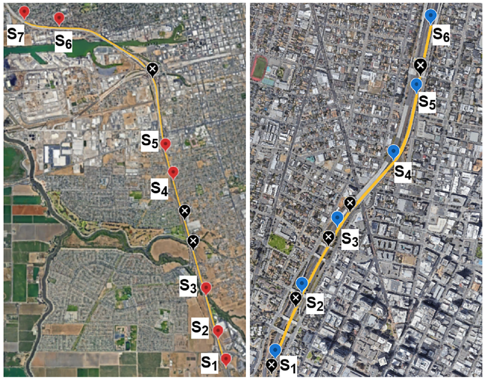
The road section of the Stockton (left) and Oakland (right) datasets.
Data Analysis
Traffic data shows both spatiotemporal correlations and periodicity. Periodicity can be seen as a long-term temporal correlation as it refers to strong repeating cycles in traffic data. These cycles could either be on a daily (different days in the same week), weekly (same day in previous weeks) or even longer time scales. Pearson’s correlation analysis is performed to identify the most relevant periodicity of the traffic data considered. The Pearson correlation coefficient

where
Long-Term Temporal Correlation Data
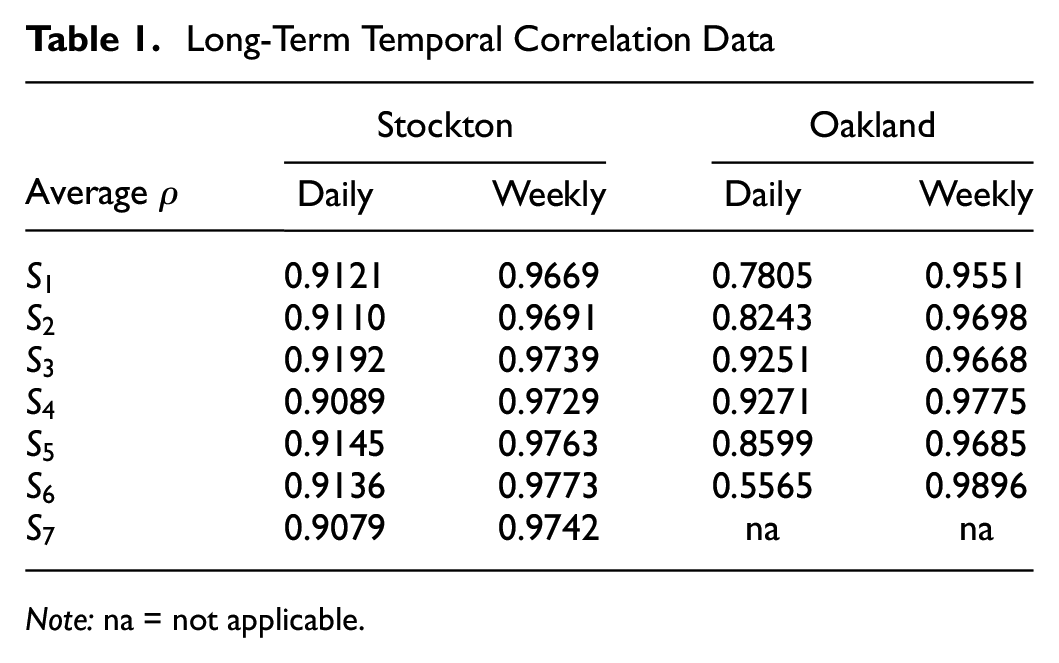
Note: na = not applicable.
Data Preprocessing
Raw traffic data usually contains missing and erroneous values, which can be caused by transmission distortion, temporary power failure, unscheduled maintenance, or sensor faults. The dataset used here contains two types of missing data: missing completely at random (nonsequential missing data) and missing at random (sequential missing data). The average of the preceding and subsequent time steps is used to replace nonsequential missing data points, while the average of the same day in adjacent weeks is used for the imputation of sequential missing data points ( 58 ).
An outlier test is performed using the interquartile range (
Problem Formulation
The traffic-forecasting problem is approached from a supervised-learning perspective. The input variables, namely current and previous traffic flows, are mapped to the output variable, representing the future traffic flow, using the sliding-window method ( 2 , 59 ). Sampling and forecasting horizon model parameters are deduced from Zheng et al. ( 11 ). As both short-term spatiotemporal and long-term temporal traffic-flow data is considered, two separate input matrices and one output vector are generated.
Inputs
The short-term spatiotemporal data is prepared as an input to the proposed model by applying the aforementioned sliding-window technique. Combining the historical traffic flow of each selected location and time interval generates the short-term spatiotemporal input, denoted
where
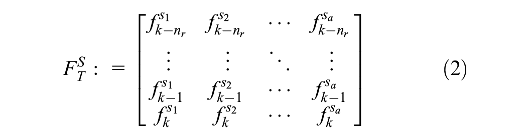
The long-term temporal data is prepared as a second input to the proposed model using the same sliding-window technique and the same output as a reference point. To account for inter-week traffic-flow variability, a time-step tolerance is added to include adjacent time steps from the past week. The resulting matrix,
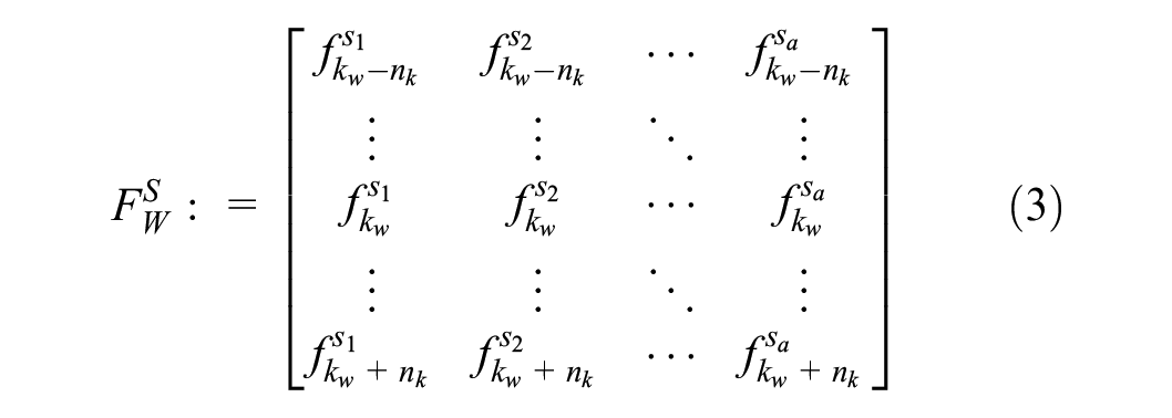
where
Output
The forecasts are calculated for each spatial location, resulting in the output becoming a traffic-flow vector for all locations in the prediction horizon

In this work, the prediction interval is set at
MIHDSAN Architecture
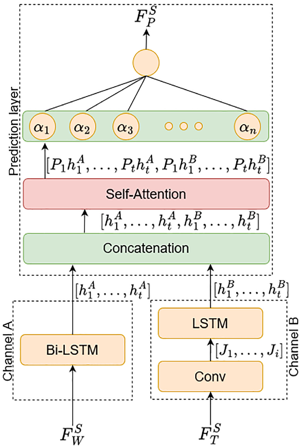
The MIHDSAN model incorporates two input channels: A and B (see Figure 2). Channel A contains a bi-LSTM layer for processing the long-term temporal data
Block model of proposed multi-input hybrid deep self-attention network (MIHDSAN).
Convolutional Layer
The convolutional layer in channel B denoted “conv” extracts the spatial features via a two-dimensional (2D) convolutional operation, which is performed over the data input

where

A pooling layer is not used here because the dimensionality of the input vector is already low. This output
LSTM Layer
The LSTM layer follows the convolutional layer, its primary function being to extract short-term temporal features from the feature maps generated by the convolutional layer. The LSTM block consists of several gates and memory units, allowing it to retain essential information and discard unimportant items. The process is as follows. First, the LSTM passes the previous hidden-state vector

The next step is to determine what new information is to be stored in the cell state. This is a two-part process. It starts with the previous hidden state


The previous cell state

Finally, the output gate of the LSTM determines what the next hidden state should be. First, the previous hidden state and cell input


where
Bi-LSTM Layer
The bi-LSTMs are an extension of the LSTM unit described previously. The difference between this layer and the traditional LSTM unit is that each bi-LSTM layer consists of two LSTM units for which the input data is fed in both the forward and reverse directions. This two-step input process improves the ability of the model to learn long-term dependencies (
60
), which will in turn improve the accuracy of the model. In this model, the bi-LSTM layer in channel A is used solely to extract features from the long-term temporal input
Self-Attention Layer
Attention mechanisms are widely used in deep-learning models to explore features inherent in data and improve the efficiency of data preprocessing. They assign attention weights to each input element in the sequence allowing the model to focus on specific portions of the input data. The proposed model has two inputs (

where

Subsequently, the computed attention weight is assigned to the corresponding input instance

where
Fully Connected Layer
The outputs from the attention layer are merged, and the resulting vector is fed as input to a fully connected neural network. This neural network consists of a single “densely connected” neuron connected to all elements in the concatenated vector from the preceding attention layer. This layer uses no activation as the problem has been fashioned as a regression problem and the values to be predicted are the numerical traffic flow for each location. The output from this layer is the scaled prediction of the model, which is subsequently unscaled to give the final prediction. The output of each neuron in this fully connected layer is computed using the following equation:

where
Experimental Settings
Performance Measures
The performance of the proposed forecasting model is primarily evaluated using the GEH statistic, an empirical measure that adeptly quantifies the deviation between predicted and actual traffic flows. The GEH is formulated as:

Given that the GEH formulation requires hourly traffic-flow data, all flow values are transformed into their respective hourly representation. Thus,
An essential aspect of the GEH statistic is its capacity to distinguish the relative importance of prediction errors, particularly across different traffic volumes. The GEH formula is structured to emphasize these differences through its mathematical formulation. The error term,
In this context, the GEH offers a more stringent criterion for higher traffic flows, where precise predictions are crucial, while permitting greater deviations in lower flow conditions. For instance, under a GEH threshold of 5, a forecasted traffic volume of
A statistic of interest is the percentage of GEH less than 5% for a given test batch. Since the data used in this study is recorded at 5 min intervals, the inherent averaging effect commonly associated with considering hourly intervals is eliminated. To overcome this potential issue, the GEH statistic is calculated for both the smaller 5 min time interval referred to as
Alongside the GEH statistic, traditional metrics such as the RMSE and the MAPE are also used for comparison. These are calculated as follows:


where
Loss Functions
The MSE and MAE are adopted as benchmark loss functions because of their widespread use in deep-learning regression tasks:


where
While MSE and MAE are quantitative measures, they do not distinguish between acceptable and unacceptable predictions. To address this, a GEH-based loss function

where
Benchmark Models
Several experiments are conducted to compare the performance of the proposed model and loss functions with the following benchmark models from the literature: LSTM ( 46 ), CNN-LSTM ( 12 ), AM-LSTM (LSTM with attention mechanism) ( 61 ) and attn-conv-LSTM (convolutional LSTM with attention mechanism) ( 11 ). The details of the model configurations are given as follows:
LSTM module: This takes in the short-term spatiotemporal data as its only input and consists of two stacked LSTM layers.
CNN-LSTM module: This module takes in only the short-term spatiotemporal input fed through two input channels. One channel extracts spatial features via a CNN, and one channel extracts temporal features via an LSTM module. These features are then subsequently fused in a fully connected layer.
AM-LSTM module: This model incorporates an attention mechanism into the LSTM network to enhance its ability to focus on critical inputs, thereby improving the prediction accuracy for short-term traffic flow. The attention mechanism helps the network assign different weights to different inputs, focusing on significant information rather than minute-to-minute fluctuations.
Attn-conv-LSTM module: The input stage consists of a convolutional LSTM module for processing short-term spatiotemporal input data, and two bi-LSTM modules for processing the daily and weekly periodicity data (defined as the long-term temporal data here). The features extracted from these layers are subsequently fused in a feature-fusing layer, which precedes two fully connected regression layers that output the final prediction. An attention mechanism as designed in the original paper is also added to the conv-LSTM module.
To ensure a fair comparison, the hyperparameters of each of the aforementioned models (including the proposed model), which include the number of filters for a convolutional layer, the number of units for an LSTM layer, and the learning rate for training convergence, are optimized using the optimization scheme detailed subsequently. In each experiment, the input lag window for the short-term spatiotemporal input is set to 15, meaning 75 min of historical data is used as the short-term spatiotemporal input for each model setup. For the attn-conv-LSTM, the lag window for the long-term temporal input is set to 1, implying that 1 day and 1 week of historical data are used to build the daily and weekly periodic input, respectively. Note that the evaluation was performed for a period not affected by holidays; therefore, the previous week exhibited similar traffic to each week considered.
Training Setup
The proposed model, together with the benchmark models (LSTM, CNN-LSTM, AM-LSTM, and attn-conv-LSTM), were developed using the Keras deep-learning API with a TensorFlow backend. Before training the models, the hyperparameters were optimized using the random search method. This method randomly combines several hyperparameters from a given parameter space to generate possible model configurations. The hyperparameters tuned in the models are given in Table 2. The optimization objective for the hyperparameter tuning is set to minimize the validation loss using the loss functions outlined in the previous subsection. The number of trials and the number of executions per trial are set to 60 and 5, respectively. The former is selected based on the recommendation by Bergstra and Yoshua ( 62 ) and the latter serves as a method to reduce the variance of the result, which occurs as a result of the random initialization of the network variables. On completion of the optimization scheme, the best hyperparameters are selected and used in the final model training, which runs for 100 epochs.
Hyperparameter Range
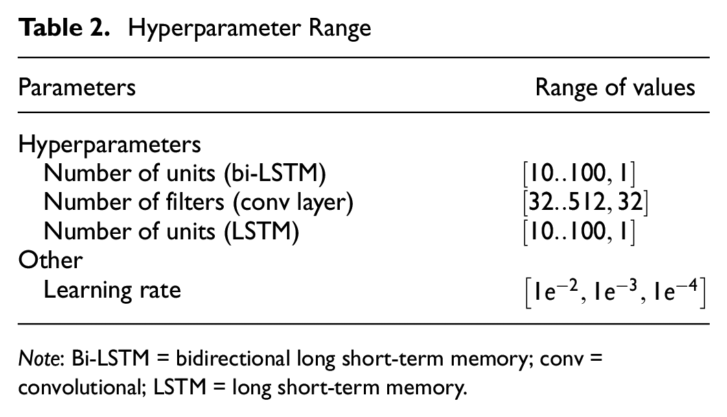
Note: Bi-LSTM = bidirectional long short-term memory; conv = convolutional; LSTM = long short-term memory.
Experimental Results
General Performance of the MIHDSAN Model
This subsection investigates the overall performance of the MIHDSAN model for multilocation forecasting on both test datasets. The forecast accuracy is presented in Table 3 as a baseline (set as the MIHDSAN model) and the relative percentage in green and red. Green values indicate better relative performance, and red indicate worse performance. The error is presented as the benchmark error measures, namely RMSE and MAPE, as well as the proposed percentage GEH for each sample, denoted
Relative Performance of Different Benchmark Models Compared with the MIHDSAN Baseline, Evaluated Using RMSE, MAPE, and GEH Metrics
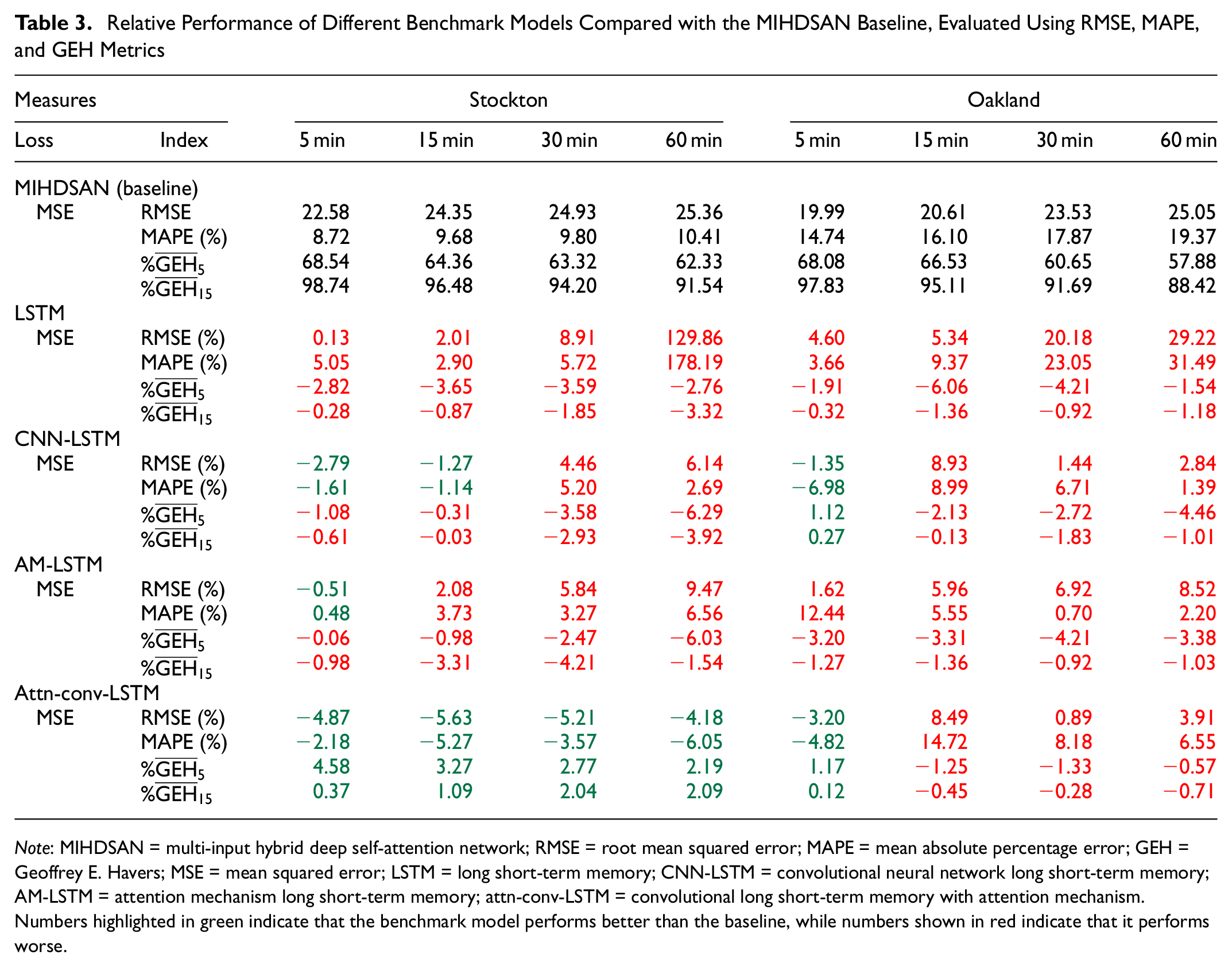
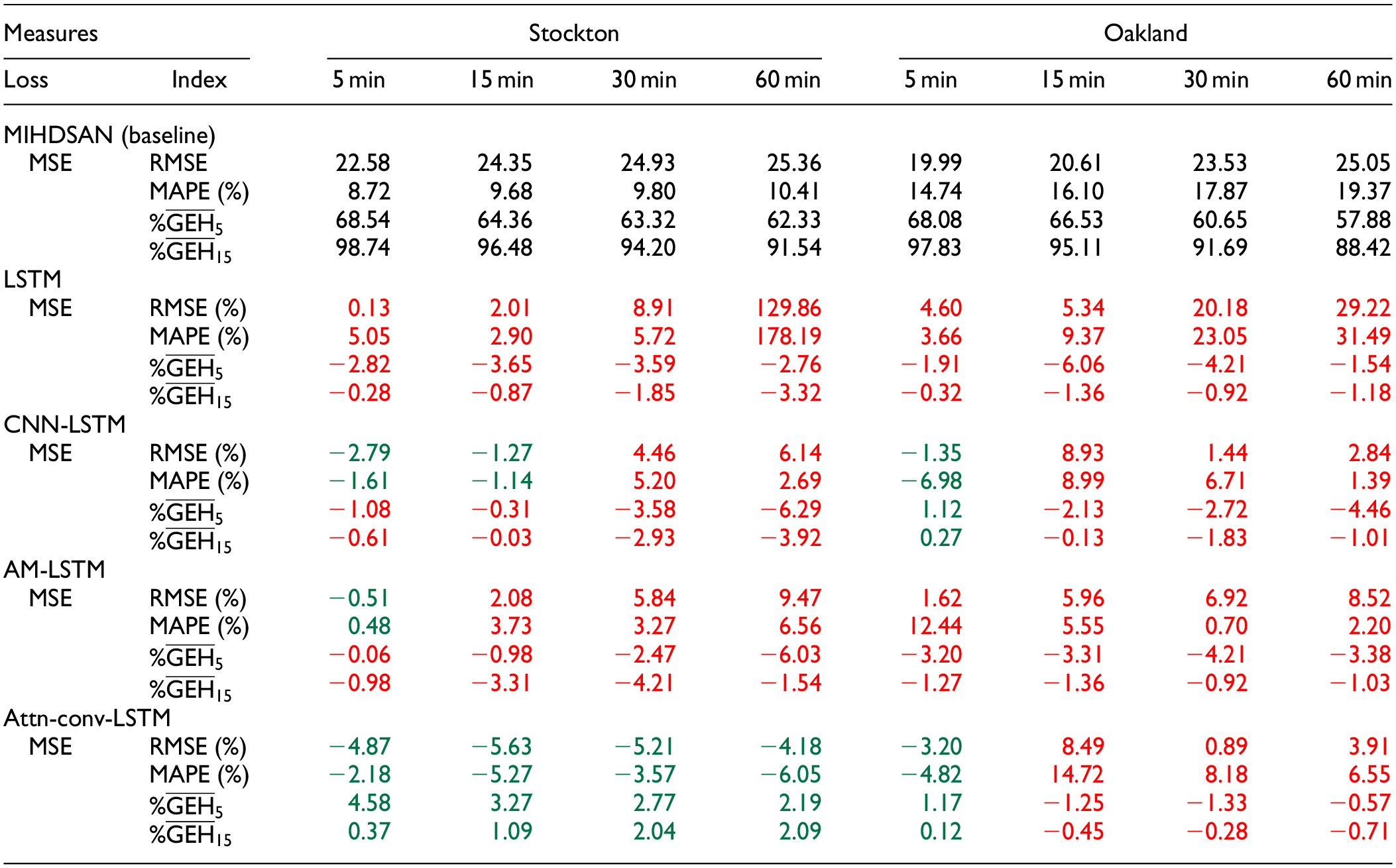
Note: MIHDSAN = multi-input hybrid deep self-attention network; RMSE = root mean squared error; MAPE = mean absolute percentage error; GEH = Geoffrey E. Havers; MSE = mean squared error; LSTM = long short-term memory; CNN-LSTM = convolutional neural network long short-term memory; AM-LSTM = attention mechanism long short-term memory; attn-conv-LSTM = convolutional long short-term memory with attention mechanism. Numbers highlighted in green indicate that the benchmark model performs better than the baseline, while numbers shown in red indicate that it performs worse.
It is observed in Table 3 that, as expected, the three-input attn-conv-LSTM and two-input MIHDSAN model outperform the AM-LSTM, CNN-LSTM, and LSTM models in most cases. This is significant for the longer forecast horizons of 30 and 60 min, confirming the benefit associated with including long-term spatiotemporal data. When the results of the three-input attn-conv-LSTM and the two-input MIHDSAN are compared, it is observed that the two-input MIHDSAN model outperforms the three-input attn-conv-LSTM in the higher forecast horizons of the Oakland dataset, while underperforming it in the Stockton dataset. These results demonstrate the need to perform a statistical analysis to identify the relevant periodic features to include in the traffic-forecasting model. Recalling the results of Table 1, with daily correlation as low as 0.56 for
The significant increase in performance when considering
Loss Functions and Evaluation Metrics
The effect of the different loss functions on the proposed model is shown in Table 4 as a baseline (set as the MSE loss) and relative percentages in green and red, with green indicating a better relative performance and red indicating otherwise. The results show that MAE and
Performance of the Proposed MIHDSAN Model under Different Loss Functions
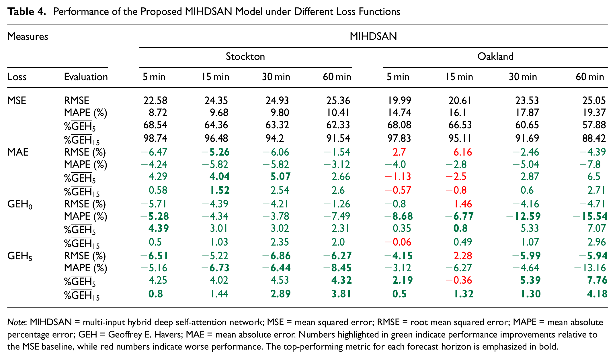
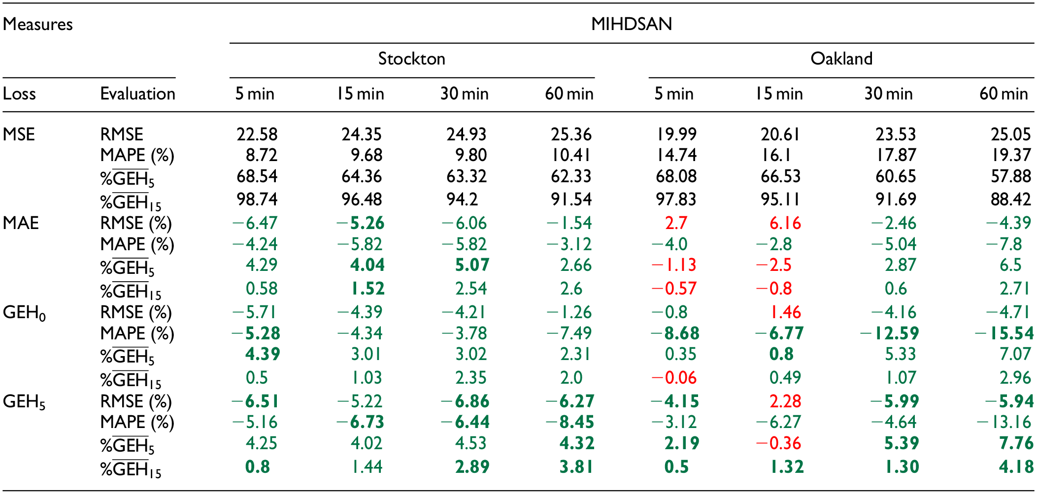
Note: MIHDSAN = multi-input hybrid deep self-attention network; MSE = mean squared error; RMSE = root mean squared error; MAPE = mean absolute percentage error; GEH = Geoffrey E. Havers; MAE = mean absolute error. Numbers highlighted in green indicate performance improvements relative to the MSE baseline, while red numbers indicate worse performance. The top-performing metric for each forecast horizon is emphasized in bold.
Therefore, in this work, to evaluate the performance of the model on individual data predictions, the suggestion is to calculate GEH for each forecast as an alternative or a complement to the prediction error. Figure 3 shows a typical 1 day prediction performance on randomly selected locations (Stockton location 5 and Oakland location 4). The top plot shows the predicted and actual traffic flow with accuracy limits determined by the GEH acceptance threshold (
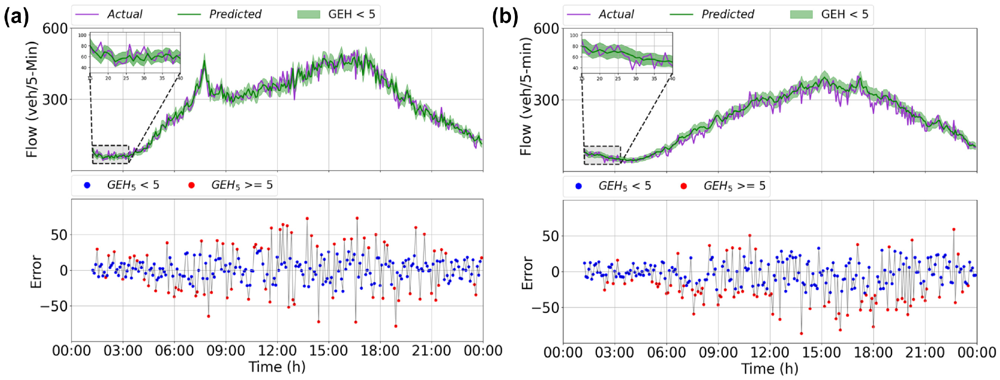
1 day prediction performance of proposed model: A comparison between prediction error and GEH to infer individual forecast acceptability (assuming
Convergence Performance of Loss Functions
This subsection compares the convergence characteristics of the MSE, MAE, and the proposed GEH-based loss functions (
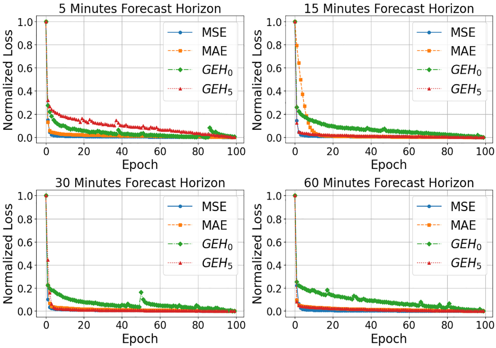
Normalized training loss convergence for various loss functions across different forecast horizons (Stockton).
MSE, MAE, and
Conversely,
The empirical evidence suggests that while
On the Long-Term Scalability of MIHDSAN
The effectiveness of traffic-forecasting models is significantly determined by their ability to adapt and scale in response to the evolving nature of urban environments. The MIHDSAN model, with its multi-input hybrid architecture, is designed with long-term application in mind, ensuring relevance even as urban traffic patterns undergo rapid changes. The modular nature of the MIHDSAN model is one of its core advantages, allowing for the integration of new data types or sources, reflecting changes such as weather conditions, policy implementations, and evolving transportation trends.
The MIHDSAN model can be easily reconfigured to accommodate additional inputs or focus on different temporal patterns as necessitated by new traffic conditions. This flexibility is important for maintaining forecasting accuracy in the face of infrastructural changes or shifts in traffic regulation. Similarly, the GEH metric, adapted for this study, presents an evaluation and loss function that can be tuned to the specific demands of the urban environment in question, offering a robust standard for model performance even when there is variability in the data.
An example of the practical application of the MIHDSAN model and GEH metric would be to provide vehicle-flow prediction for the strategic road network around Coventry, UK, as well as the three main corridors in and out of the city. This information could be used within the traffic-management software developed during the Intelligent Variable Messaging Systems (iVMS) project to equalize the traffic between the main three corridors into the city by incentivizing connected vehicles to follow specific routes based primarily on the traffic condition while also taking into account personal preferences. Traffic flows can be exploited and combined with other variables including vehicle speed, inter-vehicle spacing, traffic density within variable speed limits, speed harmonization, ramp metering, dynamic lane management, and hard-shoulder- (or all-lane-) running algorithms. Another exploitation of the MIHDSAN prediction could be to forecast the traffic over roads equipped with dynamic wireless charging to help manage the energy demand from the grid ( 63 , 64 ).
While the primary scope of this work is centered on the validation of the MIHDSAN model, the inherent potential of both the MIHDSAN framework and the GEH metric for long-term application has been demonstrated. The adaptability of the model not only serves current forecasting needs but also provides a foundation for future enhancements. As urban environments continue to evolve, the MIHDSAN model’s design can be iteratively developed, ensuring that its utility and accuracy persist over time.
Conclusion
This work has presented a multi-input hybrid deep-learning model for multilocation traffic forecasting. It has also presented the GEH statistic, which is used extensively in traffic modeling, and adapted its formulation to serve as both an evaluation metric and a parameterizable loss function for deep-learning traffic-forecasting modeling. In contrast to the benchmark model, which uses a three-input configuration, the proposed MIHDSAN model uses two inputs: a short-term spatiotemporal input and a single long-term temporal input selected via correlation analysis. Both inputs were mined by a conv-LSTM and a bi-LSTM module, respectively. The experimental results demonstrate that the proposed model offers performance similar to the benchmark and that long-term temporal inputs benefit forecast horizons beyond 15 min, improving forecast accuracy at the 30 and 60 min horizons by an average of 3%. However, it is not beneficial to use both daily and weekly temporal data if these data are not similarly correlated. In this work, the inclusion of daily data was appropriate for Stockton but not Oakland.
The proposed
While this study provides significant insights, it also opens avenues for future research, particularly in exploring the sensitivity of the model to various input features, such as different time-window sizes. Such analysis could further enhance the understanding of the model’s adaptability and robustness, potentially leading to even more refined forecasting models. This recommendation underscores the dynamic and evolving nature of traffic-forecasting research and its continuous pursuit of improved accuracy and applicability, and aids the transition toward safer and greener road transport.
Footnotes
Author Contributions
The authors confirm contribution to the paper as follows: study conception and design: M. E.; data collection: M. E.; analysis and interpretation of results: M. E., Q. L., O. H.; draft manuscript preparation: M. E., Q. L., O. H.; All authors reviewed the results and approved the final version of the manuscript.
Declaration of Conflicting Interests
The author(s) declared no potential conflicts of interest with respect to the research, authorship, and/or publication of this article.
Funding
The author(s) received no financial support for the research, authorship, and/or publication of this article.
Data Accessibility Statement
The dataset supporting the findings of this study is available on figshare with the identifier DOI: 10.6084/m9.figshare.26343748.