Sage Journals: Discover world-class research

Abstract

Despite the increasing share of nonmotorized road users, several aspects relating to modeling and planning insights have not yet been sufficiently addressed in research. The behavior of bicyclists in simulation models often differs from their real-world riding style. Therefore, to identify realistic parameters, a solid database is needed to be able to address these issues. Progressive data collection methods allow for tracking individual trajectories of nonmotorized road users and analyzing their behavior. This can then be used to improve existing modeling approaches and gain further insights. In this work, we present an analysis of cyclist riding characteristics in an urban area. A trajectory data set collected by a swarm of drones in the city of Munich was used to investigate (i) acceleration behavior after a traffic light stop, (ii) following and free-flow riding scenarios, and (iii) overtaking maneuvers. In comparison with existing studies, despite great heterogeneity among the cyclists, the overall dimensions of speed, headway, and spacing were found to be similar. In addition, it was possible to gain insights relating to the development of different parameters over time, which had been difficult to determine with previous data sources. This work therefore contributes to the common understanding of cyclists’ behavior, adding another element of bicycle characteristics to the fundamentals of modeling approaches.

Keywords

highway capacity and quality of service bicycles bicycle transportation bicycle lanes traffic operations

As a mode of transportation, bicycle traffic has progressively increased in recent years. The modal split in nearly all European cities is moving toward a higher share of sustainable, ecofriendly means of transport. Bicycle use improves health, reduces emissions and fuel consumption, and decreases traffic congestion at a low cost ( 1 , 2 ). In Munich, Germany, the modal split increased from 14% to 18% from 2008 to 2017 ( 3 ) and a new bicycle highway was recently opened connecting the suburbs and the city center of Munich. In Bergen, Norway, the world’s longest bike tunnel (3 km), Fyllingsdalen, was opened in 2023. However, in microscopic simulations of cycling, bicycles are often not modeled realistically. In existing approaches, they behave like small cars and are not represented in their variety (e.g., ranging from cargo bicycles to gravel bikes); in reality, they have less lane discipline than cars or should therefore be represented using different models. This paper aims to provide a foundation that will contribute to the modeling of cyclists in state-of-the-art microscopic traffic simulation tools. Specifically, we focused on the bicycle characteristics from free-flow riding, following behavior, and overtaking maneuvers. Based on urban drone observations at an intersection and its surroundings ( 4 ), we extracted bicycle trajectories and analyzed the riders’ behaviors.

This paper is organized as follows. First, we describe the current state of practice in bicycle parametrization. Subsequently, we introduce the study site and the collected naturalistic drone data set from Munich, Germany that was recorded in 2022. The methodology then distinguishes three cases: (a) accelerating after a traffic light stop, (b) free-flow riding and following behavior, and (c) overtaking maneuvers. The subsequent section describes the results of these scenarios, followed by a discussion and contextualization in relation to existing literature. The last section concludes the paper and gives an outlook on future research in this field.

Literature on Bicycle Parameters

Based on previous research and a commonly accepted understanding, it is apparent that there is significant heterogeneity in bicycle riding, particularly with regard to desired speeds ( 5 , 6 ). In comparison to motorized traffic, this results in more heterogeneous behavior owing to the power being provided by human beings. Furthermore, unlike cars, this behavior is not lane-bound ( 7 ). Cycling infrastructure varies greatly in relation to the presence and layout of cycle paths, and is not always favorable for cycling, for example, having to share lanes with cars or share space with pedestrians. As a result, bicyclists tend to utilize the full range of lateral options (e.g., footpaths) and even disregard traffic laws to avoid braking or stopping ( 8 ). In addition, collecting data on vulnerable road users such as bicyclists is much more difficult than for motorized traffic. However, a database—based on both microscopic and macroscopic parameters—is required for modeling, to calibrate and validate approaches. Here, we focus on microscopic parameters. Although some experiments and data collection have been carried out, microscopic modeling approaches remain insufficient for research purposes ( 9 , 10 ).

Microscopic parameters play an essential role in transport planning and infrastructure design. Several concepts to model headways and saturation flows to estimate capacity have been developed using real-world data. For instance, Hoogendoorn and Daamen used photo-finish photographs at an intersection in the Netherlands to gather headway data ( 11 ), whereas Yuan et al. used video data of a 20-m stretch of roadway to analyze bicycle trajectories ( 12 ). Other approaches include analyzing and modeling queuing behavior at intersections using video-based experimental data ( 13 , 14 ).

Field tests on saturation flow and capacity have also been carried out. Although the demand in most situations does not reach theoretical capacity, this is still of interest given the expectation of growing cycling rates. Values were found to differ depending on the infrastructure type (e.g., existence of traffic lights) and the width of the lane ( 15 ). From an experimental setup comprising 34 participants, Wierbos et al. found that a capacity of 0.475 + 1.11 ·width cyclists per second can be assumed for cycle paths with a width of more than 0.5 m ( 16 ). They also noted that the queue discharge rate for cyclists was below the estimated capacity, leading to a capacity drop phenomenon similar to that experienced by motorized traffic. Jiang et al. on the other hand did not observe such a capacity drop ( 17 ). They stated that this might have resulted from the lower speeds of cyclists compared with motorized traffic as, according to their cellular automaton model based on these data, a capacity drop was observable only at higher speeds. From their circular ring road experiment with single file movement on a 0.8-m wide path and an included on-ramp system, they observed a capacity of around 2,730 to 2,900 cyclists per hour and a critical density of 0.37 cyclists per lateral meter. Other studies have investigated capacity values ranging from 1,800 to 4,000 cyclists/(hour·meter) ( 18 – 21 ), and investigated the fundamental relations between flow and density, as well as the influence of density on riding characteristics, such as overtaking (22).

Looking specifically at modeling and simulation, Guo et al. conducted an experiment to find maximum flows and to investigate following behavior, free-flow riding, and overtaking on wide bicycle paths ( 18 ). Using an experimental study setup, Andresen et al. developed a database to calibrate their microscopic modeling approach ( 23 ). These data have further been used to examine the relationship between speed, acceleration, and other parameters such as spacing ( 24 ). Gavriilidou et al. provide guidelines for setting up such an experiment ( 25 ).

With a detailed focus on following and overtaking scenarios, real-world trajectories from the Brooklyn Bridge have been used to investigate the longitudinal and lateral distances in combination with the velocities of cyclists ( 26 ). Based on 316 following interactions and 34 overtaking maneuvers, the authors clustered the data points into subgroups to differentiate free and constrained riding, as well as identifying initiating, merging, and postovertaking stages, respectively. Similar characteristics (i.e., lateral and longitudinal distances, as well as duration and speed distribution during passing and meeting maneuvers) on a 3-m wide exclusive cycling path were investigated, although data points were only available every 0.5 s ( 27 ). Furthermore, real-world data from Stockholm were used to measure riding characteristics to improve microscopic modeling ( 28 ).

In modeling, to achieve calibration, influencing factors with a physical meaning are frequently used as parameters. Several approaches exist to describe the two-dimensional behavior of cyclists. These start with very simple approaches, such as motion equations, which do not aim for a realistic representation of cyclists. More realistic approaches include cellular automata models, social force models, utility choice models, game theoretic models, and a combination of longitudinal and lateral models, often adapted from motorized traffic ( 7 , 10 ). What most of these models have in common is that the requirement for calibration for the parameters to fit real-world data. Such parameters include desired speed, spacing and headway, acceleration and deceleration values, and interaction radii ( 5 , 7 , 9 , 29 ).

Owing to the highly diverse movement patterns of cyclists, the heterogeneity in riding characteristics ( 30 ), and the wide range of possible interaction scenarios, a sound data basis on which to determine and map both the microscopic behavior and considerations relating to the capacity of the infrastructure is still lacking. Therefore, we contribute to this database by providing a preprocessed, open-source, drone data set, and by analyzing the behavior of cyclists on an urban stretch of road including a signalized intersection. Acceleration after a traffic light stop, free-flow riding and following behavior, and overtaking maneuvers are considered and described in the next sections.

Case Study and Recorded Data

The data used for the analysis were collected in October 2022 in a highly frequented urban area in the city of Munich, Germany. Using several drones in parallel, a 700-m long stretch was recorded continuously in space and time for several hours during the afternoon peak. From the video footage, the trajectories of all road users were extracted at a frequency 12.5 fps, including information on their road user category, coordinates, velocity, and acceleration for each frame. From the available data set, the trajectories from Section I in Figure 1 were used to develop the methods and the trajectories from Section II were used to confirm the results. Further information on the data and the processing steps can be found in Kutsch et al. ( 4 ). The data are open-source for scientific purposes.

Figure 1.

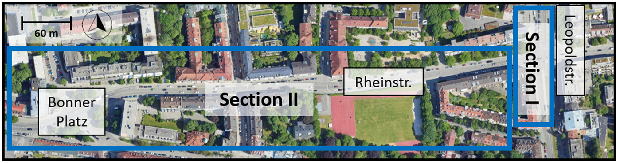
Overview of the monitoring area described ( 4 ). Methods were initially developed using data from Section I and subsequently checked using data from Section II.

From the large data set, Section I, a 140-m stretch along Leopoldstr. was selected for analysis (Figure 2a) because of the high flow volumes compared with the remaining detection area. Subsequently, the findings were verified at the eastbound area along Rheinstr. (i.e., Section II). Leopoldstr. is one of the major roads connecting the city center and the northern districts of Munich. Located near the University of Munich and several schools, schoolchildren, students, and employees alike ride there. The detailed infrastructure layout of Section II is depicted in the aerial photo taken during the drone observations (Figure 2b). At the northern part, upstream of the traffic light crossing Rheinstr., the cycle path width is around 1.35 m, directly next to the footpath, with varying width up to 2.90 m. Downstream of the traffic light, at the southern part, the cycle path width extends to 1.70 m. The cycle path is only marked off from the footpath by use of texture along the entire section. There is no curb drop or structural separation, enabling overtaking maneuvers on the footpath. Toward the motorized traffic on the riders’ left-hand side, the cycle path is separated by a curb drop and a car parking lane.

Figure 2.

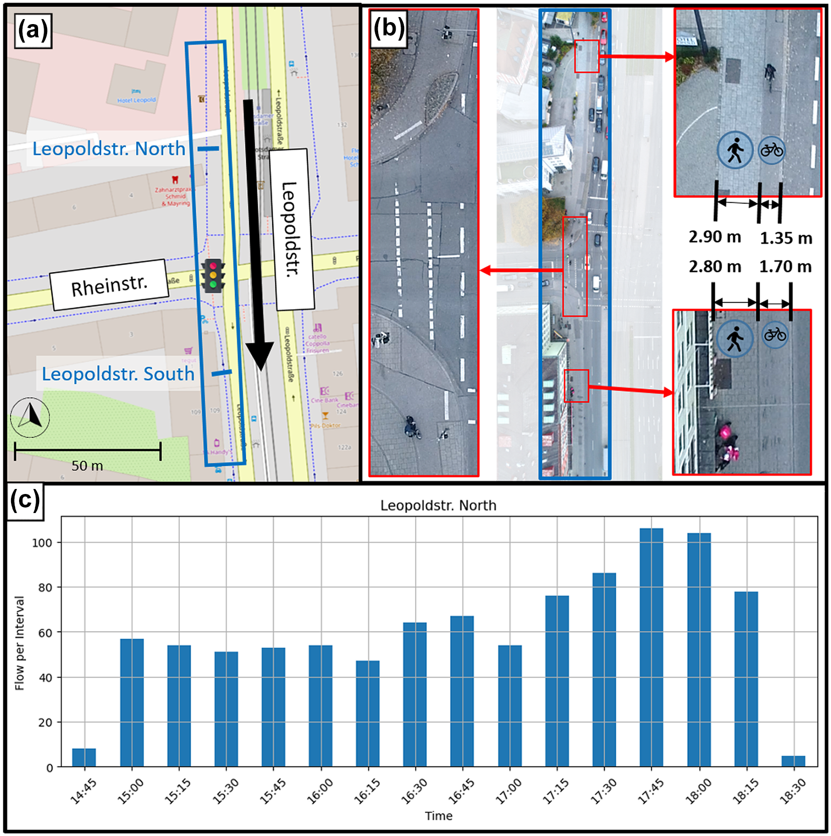
Schematic overview of (a) examined bicycle path in Munich, Germany, (b) aerial image of the section from the drone recordings, and (c) respective volumes of nonmotorized vehicles (excluding pedestrians).

This particular stretch at Leopoldstr. was chosen owing to the large bicycle volumes compared with the other sections of the study area. As Figure 2c shows, bicycle volumes are fairly high in this section, with roughly 360 bicycles/hour during peak hours. This totals 964 cyclists at Leopoldstr. North and 986 at Leopoldstr. South, with 786 traveling straight ahead (i.e., crossing both marked virtual detectors in Figure 2a) during the monitoring period of the analyzed day. As a comparison, maximum flow in Raksuntorn and Khan’s study ranged between 100 and 300 bicycles per hour ( 15 ), whereas the volumes in Mohammed et al.’s research varied from 131 to 431 bicycles per hour, on a designated cycle path without traffic light interference ( 26 ).

For our analysis, the data were spatially filtered to contain trajectories solely from within the marked area. Only bicycle trajectories were considered, however, owing to the drones’ flying altitude, no distinction could be made between normal and electric bicycles. Cargo bikes and e-scooters were excluded from the study, even though only a very small number were detected. The filtered trajectories were then processed to separate the scenarios (i.e., acceleration after a traffic light, free riding, following scenarios, and overtaking maneuvers) as described in the next section. Finally, the developed methods were applied to the cycle paths along Section II, as depicted in Figure 1, and the results were confirmed.

Methodology

To set up the data base for the different scenarios, the trajectory data were processed and partly checked by watching the videos. Filters were used, all based on the frequency of 12.5 fps.

Acceleration after Traffic Light Stop

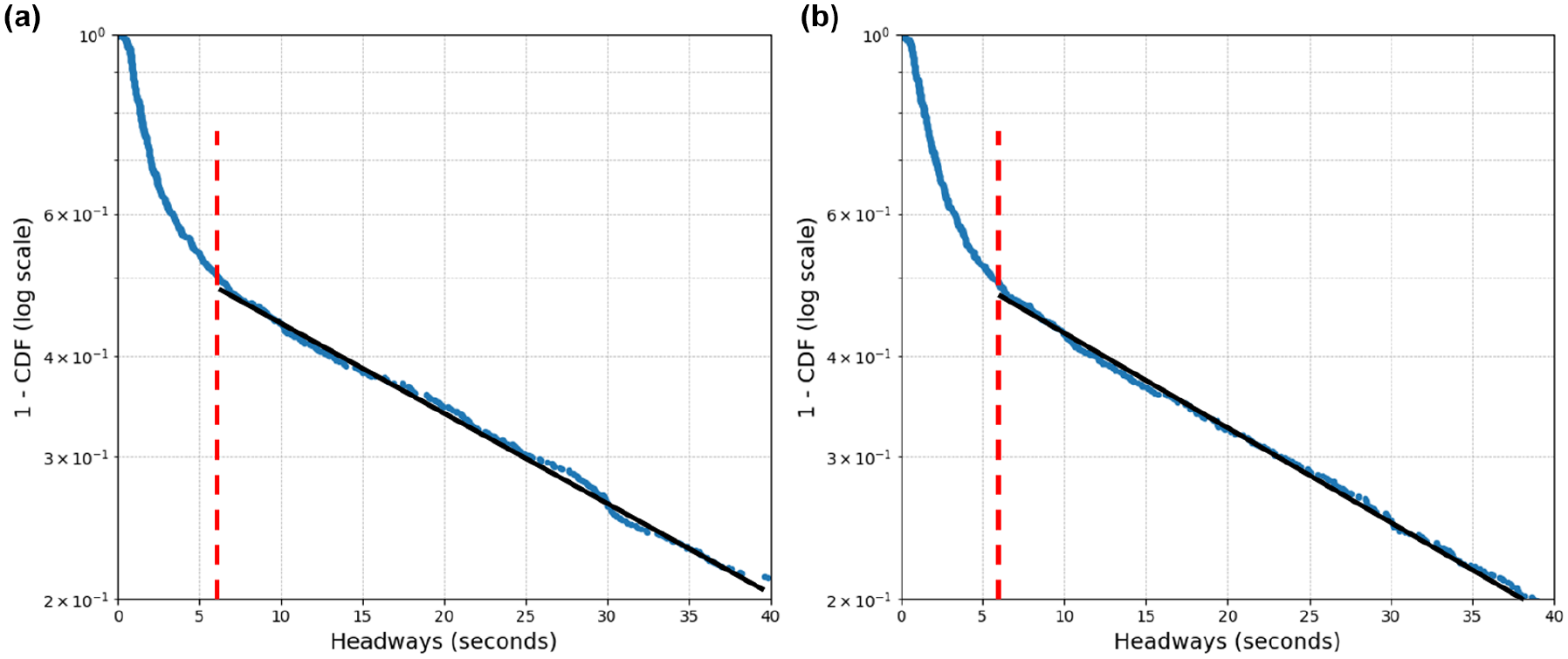
The crossing at Rheinstr. in Section I is regulated by a traffic light, separated for cyclists and motorized traffic, with the stop line being directly on the street (see Figure 2b). The aim was to analyze the free, unconstrained acceleration of cyclists after the signal had turned green. To this end, only the cyclists waiting at the front of the queue were considered, who were unconstrained throughout the remaining path southbound from the intersection. To find the threshold time gap between constrained and unconstrained riding, the graph-based method proposed by Hoogendoorn ( 31 ) and used for bicycle headway analysis by Hoogendoorn and Daamen ( 11 ) was applied. When plotting the survival function (i.e., the cumulative distribution function subtracted from 1) of all time headways between cyclists on a logarithmic scale, it becomes clear that the graph has a changing gradient up to a certain point, and then becomes a straight line. This point can be interpreted as the threshold being sought. In our data, the analysis of the headways at the northern and southern detectors (shown in Figure 2a) determined the threshold time headway to be around 5 to 6 s (Figure 3).

Figure 3.

Determination of the threshold between constrained and unconstrained riding ( 31 ) at (a) Leopoldstr. North and (b) Leopoldstr. South, as depicted in Figure 2. The threshold (marked in red) in both locations was around 5 to 6 s.

Based on this value, all starting cyclists—those at the head of the queue—following the path to the end of the section (i.e., no turning maneuvers) with a minimum time headway of 5 s until the end (i.e., 25 m, assuming a velocity of 5 m/s) were investigated for the acceleration analysis. For all starting maneuvers, the starting frame was determined, and the speed difference checked over the next time steps. In case the velocity increase in an interval with the length of 15 consecutive frames (i.e., 1.2 s) was higher than 2 km/h, the first frame of this interval was considered to be the starting frame of the acceleration maneuver. This frame was set to be Frame 0, meaning the velocity and acceleration profiles both over time and space could then be determined and compared between all start-up scenes.

Free-Flow Riding and Following Scenarios

As described in the previous subsection, the threshold value of 5 s was used to determine whether a cyclist was riding unconstrained or was affected by a leading bicycle. Together with the findings from the acceleration profile, determination of the free-riding velocities was carried out at the end of the southern part of the section, 30 m before the end of the monitored area. We evaluated each unconstrained cyclist at this point to obtain the distribution of desired speeds.

In the constrained following scenarios, a prefiltering of the data was carried out to ensure consideration of only (pairs of) cyclists that

• rode in the direction of the desired path (i.e., the mean orientation was within a certain range),

• were tracked simultaneously for at least 5 s,

• had at least one frame with an absolute distance (between the center points) less than 20 m and for all frames a maximum distance of 40 m,

• moved at least 10 m in total, and

• did not overtake each other.

As the cyclists start as a group after the traffic light stop, the investigations concentrated on the southern part of the road. The findings concerned the headway and spacing for space gaps below 25 m. It was noted that, in some cases, a bicycle trailer was detected as a second bicycle in the data, leading to really short gaps. Therefore, scenarios with a mean gap below 1 m throughout the whole tracked scenario were not considered.

Overtaking Maneuvers

Similar prefilters as already discussed were applied to determine possible overtaking scenarios. Since in previous research, interactions lasted only a few seconds (3 s on average with a standard deviation of 1.5 s, based on incomplete overtakings) ( 26 ), we set the overlap filter to a minimum of 2 s. The orientation and minimum ridden distance prefilters remained as for the free-flow riding and following scenarios. Based on the distance covered along the desired path, the remaining scenarios were checked for overtaking maneuvers. That is, at the end of the overlapping frames (in relation to time), the initially following cyclist (i.e., the cyclist initially having a greater distance to the end of the path) has a shorter distance to the end than the initially leading one.

The scenarios were then further split into a group that was affected by the traffic light during overtaking, and a group that was not. A traffic light constraint was defined in such a way that at least one of the cyclists had to reduce their speed by at least half directly before or at the stop line of the traffic light. This was double-checked by manually watching the scenarios to obtain an error-free database.

The variables for further analysis were determined in accordance with earlier work ( 26 ):

• Longitudinal distance: the distance along the path between the initially following cyclists to the initially leading cyclists (i.e., positive while the initially following is behind);

• Lateral distance: the distance between the cyclists perpendicular to the path direction (positive for overtaking on the left-hand side); and

• Speed difference: absolute velocity of the initially following cyclist minus the velocity of the initially leading cyclist (i.e., positive if the initially following cyclist is riding faster).

Note that both the velocity and the acceleration are absolute values in the riding direction of the cyclists. In addition to that, the lateral deviation from the (initially) following cyclist was calculated based on the trajectory of the (initially) leading cyclist, with reference to the wheel distance.

The trajectories were then subdivided into left- and right-hand side overtaking maneuvers (in relation to the direction of travel), based on the sign of the lateral distance. As explained in the section covering the case study and recorded data, overtaking on the right-hand side was only possible by using the footpath, which was texturally separated, without any physical barriers. This also applied to the cycle path along Section II, with the exception of the junction at the western end (Bonner Platz), where cyclists rode in a marked lane. A further distinction was made by determining whether the maneuvers were complete. Completeness refers to the course of the lateral distance: starting at a lateral distance near 0 m, going up to the maximum at (or close to) the overtaking point and, after the maneuver, reverting back to the initial lateral distance. Because of further obstacles, multiple overtakings at a time, or in the case of waiting for the traffic light, overtaking or waiting next to a queue, cyclists also did not swerve out before the considered overtaking maneuver (i.e., the lateral distance was not close to zero at the beginning), did not merge in afterwards, or both.

This classification was based on the assumption that the starting and ending points of an overtaking maneuver were known. These points were determined based on the lateral distance and time relative to the overtaking point. An overtaking point here refers to the frame (in time) at which the initially following cyclist first had a smaller distance to the end of the path than the initially leading rider (i.e., the longitudinal distance turned negative). To compare all overtaking maneuvers, this frame was again set to be the reference frame (i.e., Frame 0). Then, the steps shown in Figure 4 were carried out to find the starting point of the maneuver.

Figure 4.

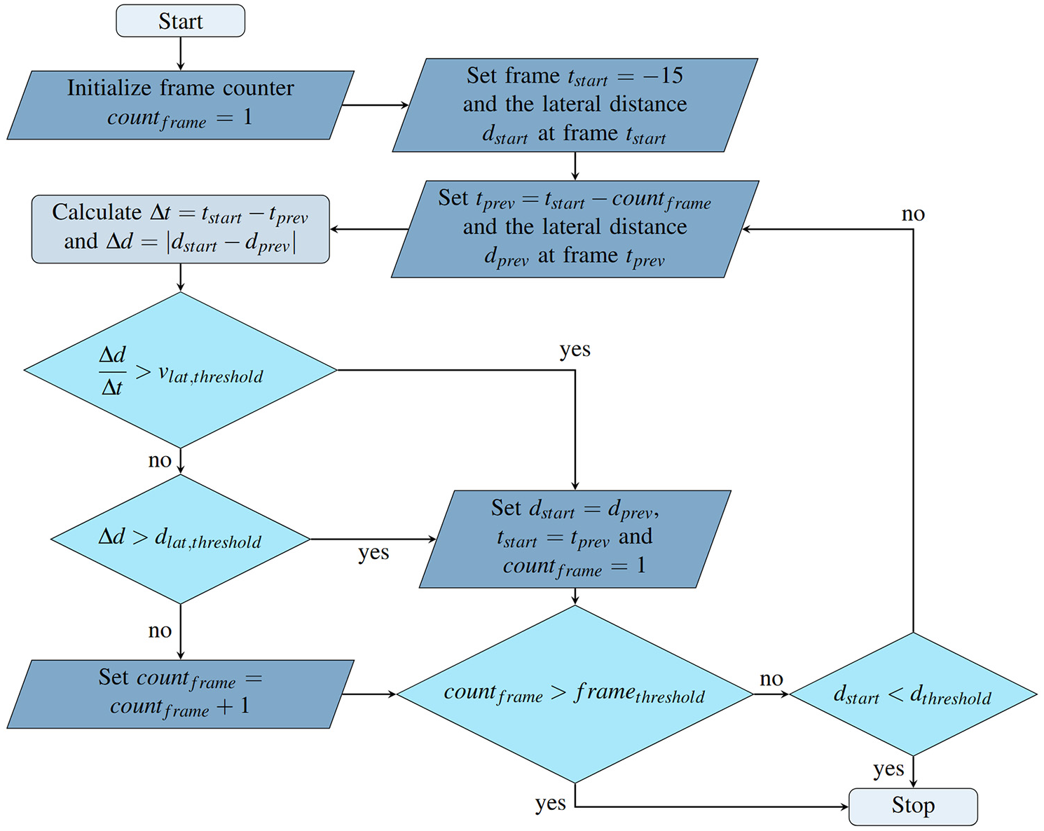
Process for determining the start frame of an overtaking maneuver.

The respective threshold values for the parameters were determined manually. We selected the following limits:

• Lateral speed, $v_{lat, threshold}$ , of 0.125 m/s,

• Absolute lateral distance threshold, $d_{lat, threshold}$ , of 0.2 m,

• Upper limit for the frame count, $fram e_{threshold}$ , of 15 frames; and

• Absolute distance threshold, $d_{threshold}$ , of 0.05 m.

This process was repeated for the end point of the overtaking maneuver. From trying different threshold values and checking the results manually, the threshold values for determining the end of the maneuver were found to be slightly different: the ratio of the difference of the lateral distance, Δd, and the time difference to the currently set starting point, Δt, (i.e., $v_{lat, threshold}$ ) needed to be set to 0.0625 m/s and the stop condition for the frame counter $fram e_{threshold}$ was chosen to be 18 frames.

Figure 5, a to d , show four examples of the resulting start (in orange) and end (in green) frames: (a) illustrates a complete, unconstrained left overtaking, (b) a complete, unconstrained right overtaking, (c) an incomplete (i.e., not merging afterwards), unconstrained left overtaking maneuver, and (d) a left overtaking maneuver after the stop at a traffic light, where the overtaking cyclist was waiting next to the queue.

Figure 5.

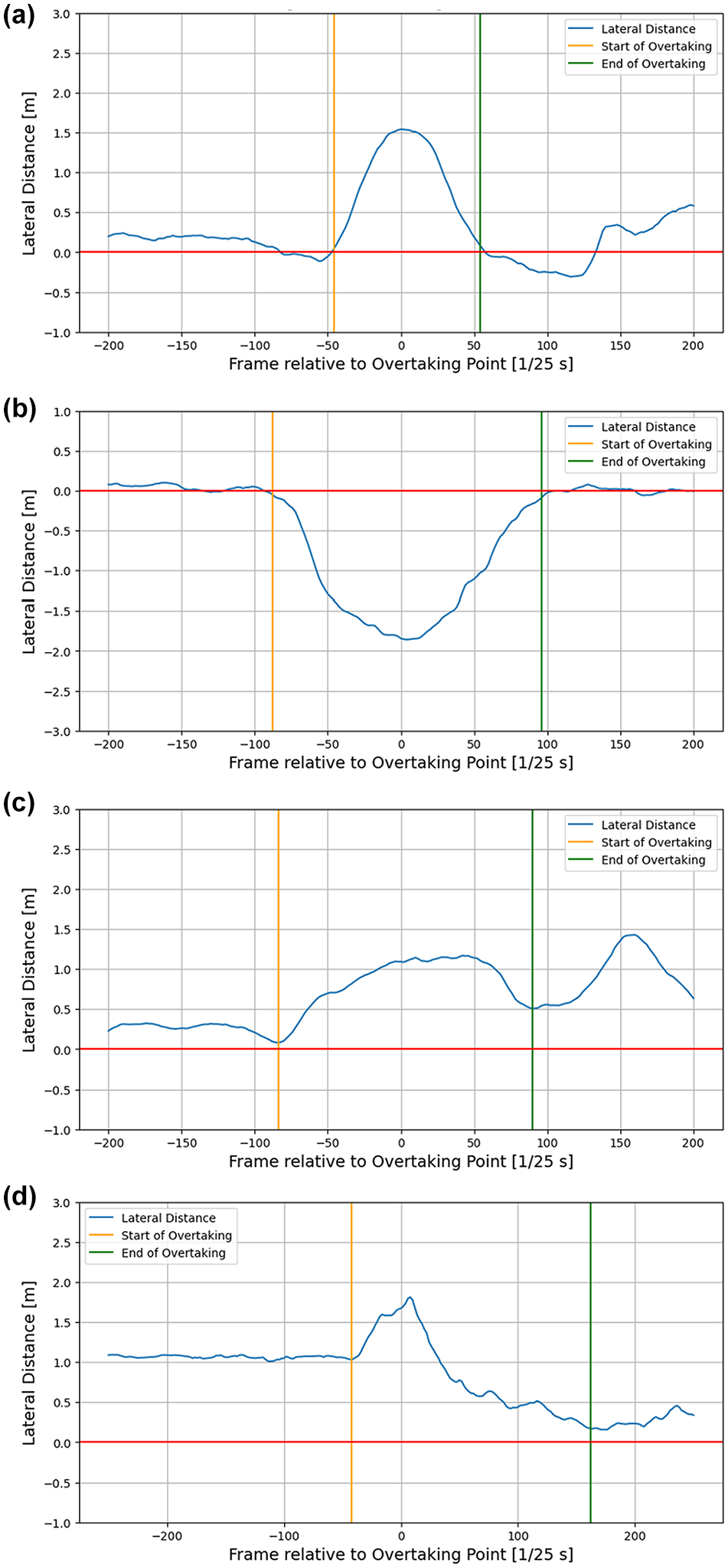
Lateral distance between pairs of cyclists during an overtaking maneuver: (a) complete left-side overtaking, (b) complete right-side overtaking, (c) incomplete maneuver, and (d) overtaking cyclist waiting next to the queue.

Results

This section presents the results of the three scenarios analyzed.

Acceleration after Traffic Light Stop

The filter described above resulted in a total of 98 starting maneuvers with which to analyze the acceleration behavior in Section I. This number was reasonable considering the total amount of roughly 200 min recording time, varying cycle lengths (actuated control) of around 90 s and rare left-turn maneuvers after the intersection. Furthermore, constrained accelerations may occur from other road users coming from the western cycle path, where right-turning cyclists do not have to stop during the green interval of conflicting streams.

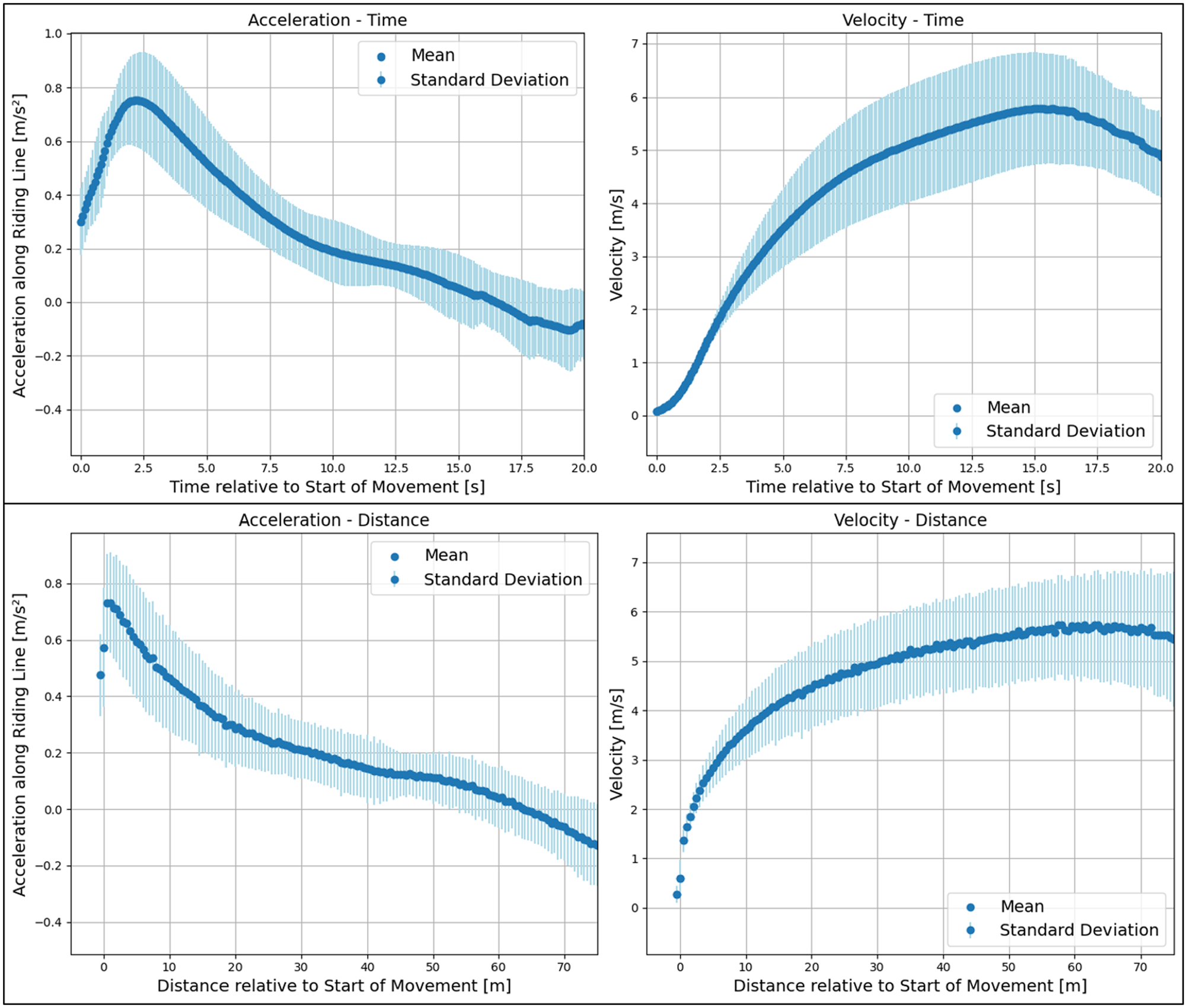
When looking at the mean acceleration relative to the starting point as described, the maximum was reached after 2.16 s with a mean acceleration of $0.75 m / s^{2}$ and a standard deviation of $0.18 m / s^{2}$ . The fastest accelerating bicyclist produced a value of $1.23 m / s^{2}$ . After the starting point, acceleration decreased to around 15 s. The mean maximum velocity then was 5.7 m/s (standard deviation: 1.54 m/s, minimum: 3.35 m/s, maximum: 8.07 m/s), as visible in Figure 6.

Figure 6.

Mean acceleration and the mean velocity for undisturbed starting scenarios after a traffic light (i.e., the first cyclist in the waiting queue) over time and space from 98 starting maneuvers.

When comparing the acceleration over the ridden distance, it was noted that the maximum after 2.16 s corresponded to a ridden distance of only 1.5 m and the maximum velocity was reached at a distance of around 60 m after the stop line (approx. 10-m south of the marked detector at Leopoldstr. South in Figure 2a). Maximum acceleration was reached at a velocity of around 1.5 m/s.

Slightly higher acceleration values were found for the unconstrained accelerations at Bonner Platz in both directions along Section II. Here, 37 and 39 cyclists starting unconstrained after a red light in each direction, respectively, were observed. This again was a reasonable amount, considering the cycle times and the lower bicycle volumes. These higher acceleration values resulted in smaller time intervals to reach maximum speed. The mean value here was around 12 s.

Free-Flow Riding and Following Scenarios

From the results of the previous section, the maximum speed (i.e., the speed that cyclists intended to ride at), was reached around 60 m after the stop line. Furthermore, the threshold headway of 5 s was adopted. With an assumed speed of 5 m/s, these 5 s would result in a threshold of 25 m. Therefore, the free-flow speed was determined at the southern part of Leopoldstr., in the section 35 to 25 m before the end of the observed area. It was assumed that the cyclists not affected by the traffic light reached their maximum speed here as well, although they might have reached this speed earlier. The mean speed of the 433 observed free-flow riding cyclists was 5.24 m/s with a standard deviation of 1.34 m/s. The measured minimum velocity was 2.01 m/s, whereas the maximum speed was 8.40 m/s.

The spacing and the headway distributions of the following scenarios investigated can be seen in Figure 7. Spacing refers to the gap between the center points of the cyclists along the riding path, and the headway is the calculated time that the following cyclist would need to close this gap (i.e., between the center points) at current speed (assuming that the leading cyclist immediately stops moving). The mean value of the space gap per scenario was found to be 9.58 m, ranging from 1.07 to 22.85 m. Please note that these distances refer to measurements in which the calculated headway was less than 6 s (which refers to the determined threshold value as depicted in Figure 3). Since the mean spacing did not take into account the current speed of the cyclists, headways were also considered. The mean value for the scenarios was found to be 1.96 s, but with a comparatively high standard deviation of 1.21 s.

Figure 7.

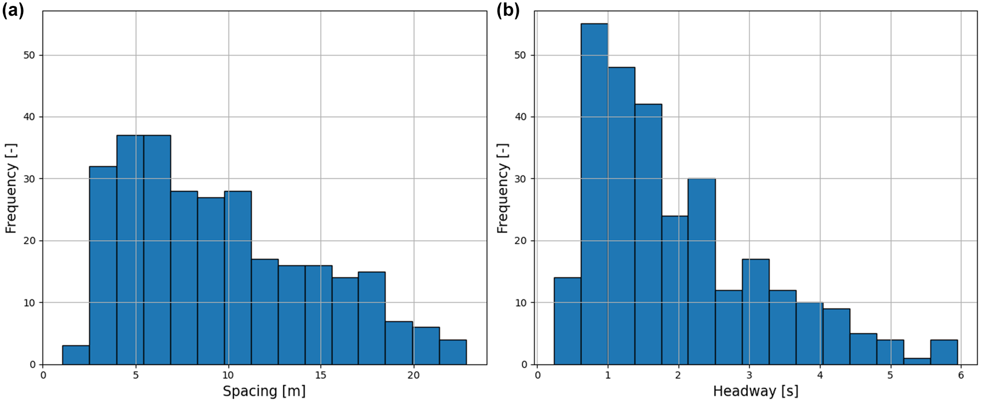
Histograms of (a) the space gaps and (b) time headways for the mean values of each following scenario.

Overtaking Maneuvers

As detailed in the methods section, we first separated the overtaking maneuvers into free overtaking and maneuvers constrained by traffic lights. A distinction was also made between left and right overtaking maneuvers, as well as between complete and incomplete maneuvers with regard to lateral riding behavior. Complete overtaking in that sense means that the initially following cyclist starts at the same lateral level behind the preceding cyclist, such that the lateral distance is close to 0 m. The cyclist then swerves out to a maximum lateral distance (roughly) at the overtaking point and afterwards merges into a lateral distance close to 0 m again. Incomplete overtaking, on the contrary, refers to an overtaking maneuver where either no swerving before, no merging afterwards, or both are observed. These observations resulted in a total of 179 maneuvers at Section I and 140 along Section II, as can be seen in Table 1. A further 63 scenarios were detected, but owing to the maneuver being too close to the beginning or end of the monitored section, they could not be followed from start to end, and were therefore excluded from the analysis.

Table 1.

Overtaking Maneuvers

Type			Section I	Section II
Free/undisturbed	Left	Complete	25	36
	Left	No swerving or merging	19	30
	Right	Complete	11	42
	Right	No swerving or merging	8	12
Traffic light impact	Left	Complete	35	8
	Left	No swerving or merging	41	10
	Right	Complete	6	2
	Right	No swerving or merging	34	0
Missing start or end of the maneuver			51	12

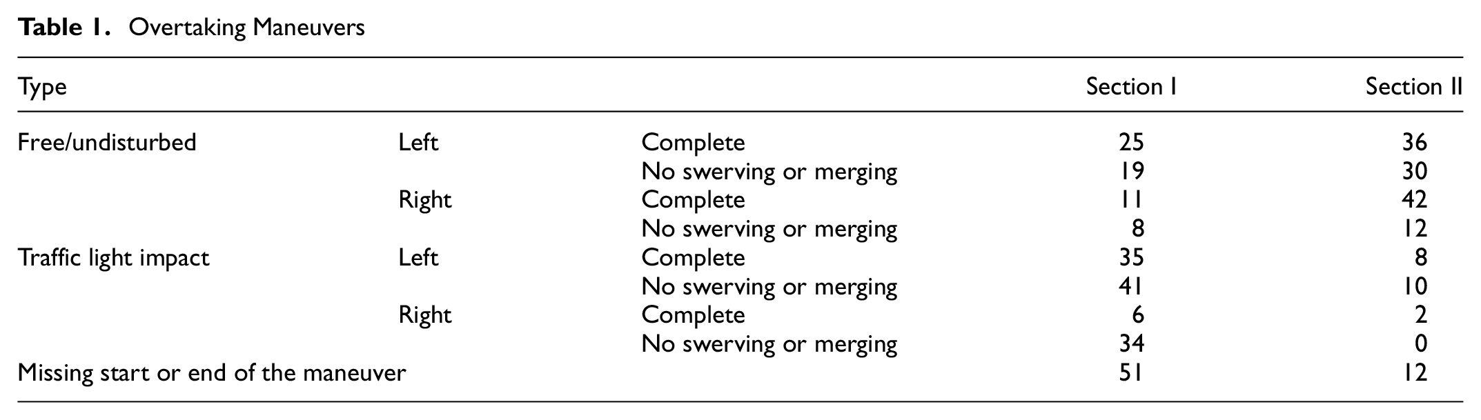
Figure 8 depicts the overtaking points. For maneuvers affected by traffic lights (Figure 8a), the majority of overtaking maneuvers happened during or shortly after the red interval in front of the stop line. The whole width of the bicycle path, as well as the footpath, were almost equally used here. For the free-flow overtaking scenarios (Figure 8b), right-hand side overtaking mainly occurred at the northern part of the section. There were even more right- than left-hand side passes undertaken on this stretch. The width of the footpath compared with the cycle path was comparatively broad, especially when considering the widths on the southern part of the road. Therefore, in both cases, almost all of the maneuvers downstream of the traffic light were left-hand side overtakings. Overtaking was also predominantly on the right-hand side along Rheinstr. if there was sufficient space on the footpath. However, the overtaking maneuvers at the traffic lights at Bonner Platz were different: because of the structural separation between the cycle lane and footpath, overtaking here was almost exclusively on the left.

Figure 8.

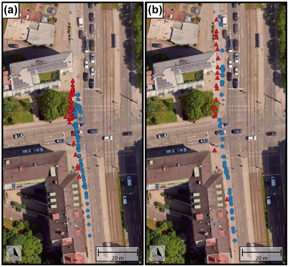
Locations of the overtaking points: (a) maneuvers affected by traffic lights, and (b) unconstrained overtaking. Only the position of the initially following cyclist is shown for left-hand side (marked as blue circle) and right-hand side (marked as red triangle) overtaking maneuvers.

Analysis of the overtaking scenarios encompassed the speed differences and lateral distances before, during, and after the maneuver, as well as the duration and the length ridden until the scenario was completed. To ensure reliable assumptions, especially with regard to the last two points, the beginnings and endings need to be determined as exactly as possible. The aforementioned method allowed for a clear distinction to be made when a complete overtaking maneuver was executed. However, in the case of incomplete settings, it was often challenging or even impossible to determine the precise location of these points. This became clear when considering a cyclist overtaking several cyclists in a row. It was almost impossible to separate when one overtake was finished and the next one started. Therefore, only complete passes were considered for the duration- and start/end analysis.

Figure 9 shows the course of the mean values of the lateral distance, speed, and acceleration with regard to the time relative to the overtaking point (Frame 0) at Section I. It can be seen that the mean lateral distance between the interacting cyclists in a left-hand side overtaking was at its maximum of 1.33 m about 0.5 s after the overtaking point. The standard deviation at this point was 0.62 m. In comparison, the maximum lateral distance for right-hand side overtaking was also reached shortly after the actual overtaking point, with an absolute mean value of 1.51 m and a lower standard deviation of 0.38 m. Similar values were found for the overtaking maneuvers at Rheinstr. (i.e., a maximum mean distance of 1.25 m shortly after the overtaking point for left-hand side maneuvers, and 1.22 m on the right-hand side, where the footpath was narrower than at Leopoldstr.). Note that this was the mean value of both scenarios, respectively: unconstrained and traffic light–constrained. Breaking down these two groups once again, it becomes clear that the maximum mean lateral distance (mean 1.11 m, SD 0.26 m) was lower for free-flow left-hand side overtaking than the traffic light–constrained maneuvers (mean 1.39 m, SD 0.63 m).

Figure 9.

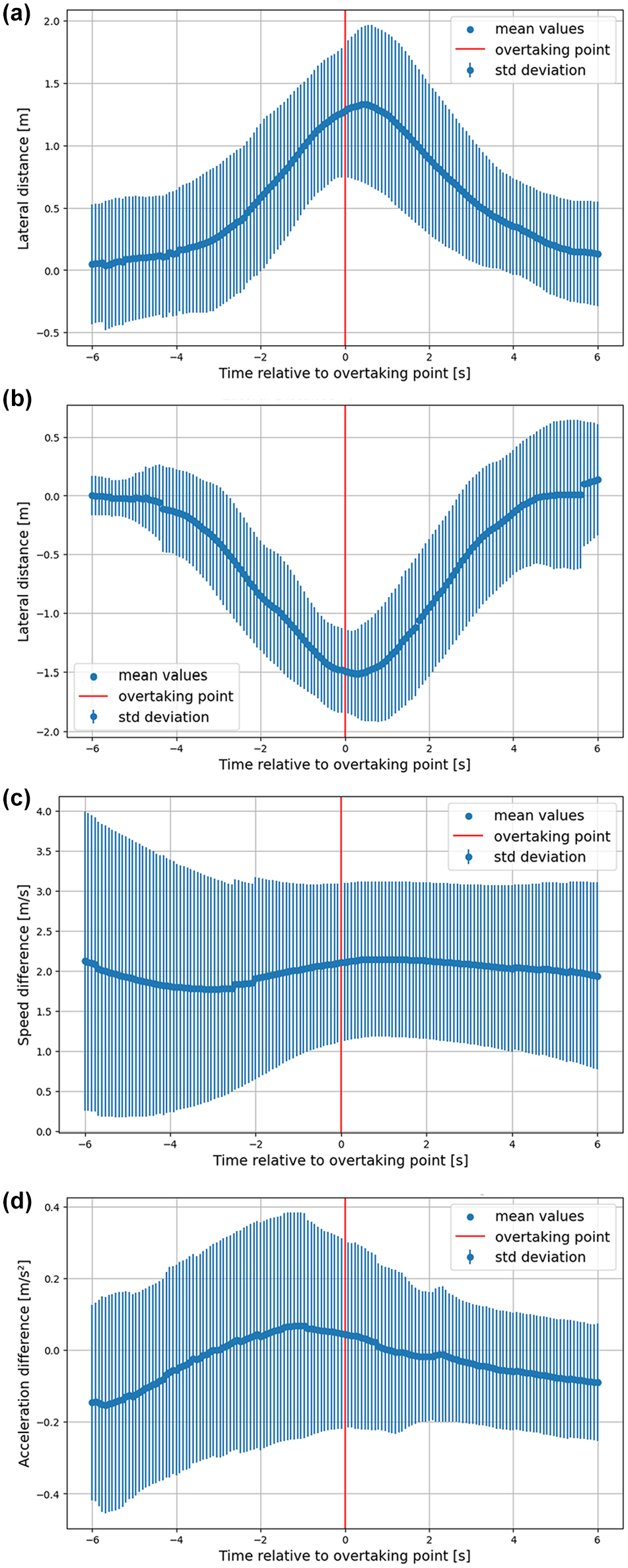
The mean values and standard deviations of the lateral distance in dependence of the relative time to the overtaking points for (a) left-hand side and (b) right-hand side overtaking maneuvers. For left-hand side overtaking, (c) the speed difference and (d) acceleration course are shown.

Along Section I, the mean value of the starting point of left overtaking maneuvers was 3.81 s (SD 1.39 s) before the overtaking point, and about the same period for right overtaking maneuvers. Cyclists then took longer to complete the maneuver and merge afterwards, giving a mean value of 4.17 s. This was consistent with the finding that the maximum lateral distance was only reached shortly after the overtaking point. The resulting mean duration of the overtaking maneuvers amounted to 7.99 s (SD 2.39 s) and 8.27 s (SD 3.39 s) for the left and right overtaking maneuvers, respectively. The mean distance required for an overtaking maneuver was 40.68 m (SD 17.52 m). Similar values were found for the overtaking scenarios along Section II, except for the difference before and after the overtaking point, where the intervals were roughly equal.

The generally high standard deviation values confirmed the previously described assumptions that the heterogeneity of cyclists’ riding characteristics was high. This becomes even more apparent when looking at the speed differences during overtaking (see Figure 9c) and the acceleration values (Figure 9d). The mean speed difference when the overtaking maneuver began was 1.76 m/s, but it had a standard deviation of 1.33 m/s. This can be explained by the traffic light–constrained overtaking. Cyclists in motion overtaking a queue had greater speed differences. The mean difference at the end of the overtaking was slightly lower than in the beginning, with a mean of 1.69 m/s. Looking at the course of the speed and the acceleration, the overtaking cyclists tended to slow down a little when starting the overtaking phase (e.g., an over-the-shoulder glance behind them). When swerving out and shortly before the overtaking point, the acceleration was at its maximum. After this point, the acceleration went down again and fell back to negative values (i.e., cyclists revert to their initial speed before the overtaking maneuver). The same shape for the speed and acceleration curves was observed along Section II, although a smaller overall difference in speed was observed.

Discussion and Comparison with Previous Findings

In most cases, the examined parameters aligned with the findings of previous research. The value of 5 s as the threshold between constrained and unconstrained riding found in this study equaled that found by Mohammed et al. ( 26 ) and was a little higher than what was found by Hoogendoorn and Daamen (4 s was chosen as the threshold, although only around 2 s was measured using the same method) ( 11 ). Twaddle and Grigoropoulos also used 2 s to differ between following and unconstrained riding, but this value was based on an assumption ( 32 ).

Based on our threshold, the free-flow speed in our data was determined to be 5.24 m/s, with a standard deviation of 1.34 m/s. The minimum speed was 2.01 m/s, whereas the maximum was 8.40 m/s. Note that it was flat terrain, sunny October weather, and there was almost no wind during recording. Castro et al. summarized several studies, which resulted in a free-flow riding speed range of 4.7 to 6.9 m/s (SD 1.1 m/s) ( 28 ). They observed a mean speed of 5.83 m/s on flat terrain (and 4.52 m/s for an uphill slope). Twaddle and Grigoropoulos found a mean free-flow riding speed of 5.23 m/s (SD 1.25 m/s: minimum: 4.20 m/s, maximum: 6.02 m/s) at several intersections in Munich ( 32 ). The slight variation in the values found across studies might result from different infrastructure, distinct riding behaviors in different countries, and varying shares of electric bicycles. However, the consistency of our findings with the literature was fairly good, especially when taking into account the previously determined values for Munich.

Typically, when considering following behavior, spacing and headways are determined. Measuring headways is often done using the concept of virtual sublanes ( 11 , 12 ). As we prefiltered the following maneuvers so that only the following scenarios were considered, where for at least 95% of the time steps the rank difference along the desired path was exactly 1 (i.e., the follower rode directly behind the leader), there was no need to apply this concept. To support this hypothesis, we also tested determination of the headway with varying virtual widths of 1.0 to 1.40 m (stated to be reasonable [ 12 ]), which produced the same distributions. Furthermore, we did not consider one crossing line or detector, but the currently ridden speed and the space gap to the preceding cyclists. The mean value for the calculated headway in our data was found to be 1.96 s, with a high standard deviation of 1.21 m. For the investigated sublane widths of 1.0 to 1.40 m, the mean headway resulted in values ranging from 1.84 to 1.61 s and standard deviations around 1.0 s ( 12 ). Another influence investigated by Yuan et al. that we did not consider was the queue discharging process ( 12 ). Therefore, the slightly higher mean headway in our calculation seemed reasonable. For the space gaps in the following scenarios, the values ranged from 1.07 to 22.85 m with a mean value of 9.58 m. These mean space gaps were fairly close to the values found by Mohammed et al. (i.e., mean: 9 m, min: 1.5 m, max: 24 m) ( 26 ).

The results for acceleration from standstill after a traffic light were partially consistent with the values from existing literature. Andresen et al.’s research determined that the maximum speed was reached after 20 to 25 m after standstill, taking around 7 s to attain the maximum speed of 4.3 m/s ( 23 ). This differs considerably to the values from the observed scenarios in our data, where the maximum velocity on average was reached at 60 m and 15 s after the start along Leopoldstr. On the other hand, Castro et al. summarized studies and found a mean acceleration of between 0.3 and 0.4 $m / s^{2}$ and maximum accelerations of 0.7 to 1.0 $m / s^{2}$ , which is consistent with our findings ( 28 ). By building a mean acceleration over the first 15 s after the starting frame in our data, a value of 0.36 m/s² resulted. The maximum acceleration was measured at 1.23 m/s². However, in the literature, the distance and speed when the maximum acceleration was reached (3.6 to 5.75 m and 2.1 to 2.8 m/s [ 28 ]) are slightly higher than in our data (1.5 m after the starting point at 1.5 $m / s$ ).

There may be several reasons for the difference in time and distance to reach maximum speed between previous studies and this work. Firstly, lower free-flow speeds were determined in an experimental setup in Andresen et al.’s research ( 23 ). In further studies in which the measuring range was constrained spatially, the maximum speed was probably not reached within the measured area (i.e., with acceleration from standstill). In our data, for instance, the distance and time up to 4.3 m/s was attained after 20 m and 7 s, respectively, which aligns precisely with Andresen et al.’s observations (23).

A second reason might be the influence of infrastructure design (i.e., path type and width, curvature, and minor aspects such as the curb height when crossing the road). At Bonner Platz, where there is a marked bike lane in both directions, the time span was 3 s shorter. To verify this, three other intersections from a drone-based survey in Ingolstadt, Germany were examined using the same methodology. The infrastructure at all three intersections was straight and comprised separate bicycle paths. The results showed similar accelerations and an average time of 11 to 12 s to reach the desired speed.

A further impact on the queue discharge rate can be the density of the queue. In previous studies, denser waiting queues led to higher discharge rates ( 14 ). To test the effect on the acceleration behavior of the respective first cyclist, the influence of the waiting queue length (i.e., the amount of cyclists in the queue) on the mean acceleration and maximum velocity is shown in Figure 10. The fitted linear regression shows that longer waiting queues tended to have a positive impact on the acceleration of cyclists, although neither the slope nor the R² values were particularly high.

Figure 10.

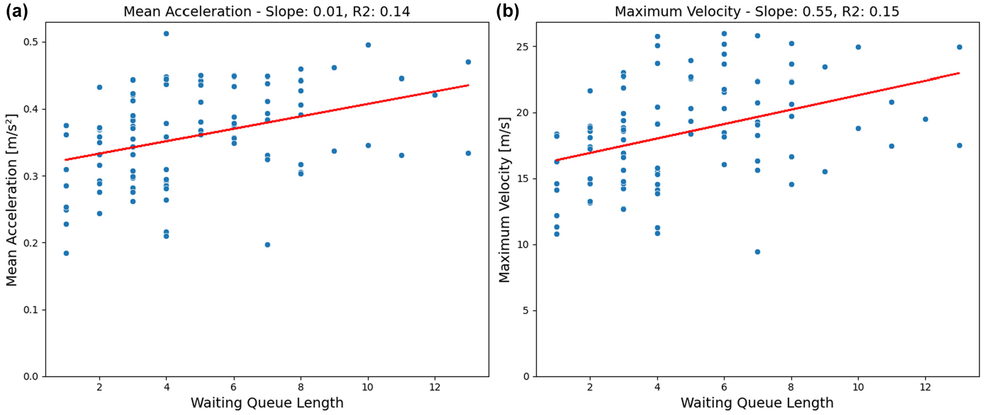
(a) Mean acceleration and (b) maximum velocity of the respective first cyclist in a waiting queue depending on the queue length. The results of a linear regression model are shown in red.

Finally, various other aspects such as the general density on the cycling infrastructure, pedestrians, and other road users, trip purpose, and the composition of cyclists in relation to both vehicle type and personal preferences might influence these values. These aspects were beyond the scope of the current investigation, and remain for future research.

For overtaking maneuvers, mainly the lateral distances, the speed differences between the overtaking cyclist and the initially leading cyclist, and the length are available from the literature. Although the speed difference of 1.2 m/s found by Mohammed et al. ( 26 ) is smaller than the value in our data set (1.76 m/s on average), the value for other locations (e.g., Khan and Raksuntorn [ 27 ]) of 2.6 m/s was higher. Reasons for that might again be the different types of infrastructure, different riding behavior in Germany compared with other countries, and the general heterogeneity among cyclists. It is reasonable to assume that lateral distances will depend on the available space. Even when comparing the left- (1.33 m on a path width of 1.35 to 1.70 m) and right-hand side (1.51 m on a footpath width of 2.80 to 2.90 m) overtaking maneuvers within our data, the average difference was almost 20 cm. This assumption is also stated in previous research. After clustering, Mohammed et al. obtained an average lateral distance of 1.51 m in the initiation phase for a path width of 2 m ( 26 ). Khan and Raksuntorn determined an average maximum lateral spacing of 1.88 m for a 3-m wide cycle path ( 27 ). Finally, the mean length of 40.62 m found in the current research was in accordance with earlier measurements and assumptions, in which the lengths varied from 24 to 91 m on 1.80- and 3-m wide cycle paths (27).

Conclusion and Outlook

Despite the increasing number of cyclists, some aspects of modeling and infrastructure planning for nonmotorized road users have not yet been sufficiently researched. However, to gain meaningful insights and challenge current microscopic modeling approaches, a wealth of fundamental data are required.

In the presented work, we have given an overview of various bicycle riding parameters that were analyzed from urban trajectory data collected using drones. The determined microscopic value distributions during different scenarios, namely accelerating after a traffic light stop, constrained following movement, unconstrained riding (i.e., free-flow conditions), and overtaking maneuvers, were then compared with findings from previous experiments and data collection results.

Most of the determined parameters aligned with the findings in previous research. Free-flow riding velocities, space gap and headway distributions, as well as lateral distances and speed differences during overtaking maneuvers only varied slightly from previous observations. These small deviations can be explained by the infrastructure layout, different cycling behavior depending on the country, and the generally large heterogeneity among cyclists. These factors may also have played a role in explaining the differences in acceleration behavior. In our scenarios, the distance until the maximum speed was reached was significantly greater than that described in the literature. The influence of further parameters on the acceleration behavior, such as the queue density or the composition of the fleet, remains open for future research.

Moreover, further insights could be gained from the highly detailed data set, both in relation to temporal resolution and data quality. These mainly concern the temporal course of processes (in relation to lateral distance, speed, and acceleration) involved in overtaking maneuvers and the time headways and space gaps that cyclists maintain during following scenarios. Investigating these gaps, especially with regard to the temporal course and in dependence of speed will be subject to future research.

It should be mentioned here that the data represent a local analysis in a major German city. The results from other countries could differ because of different riding behavior. It should also be noted here that the data set does not explicitly contain congested bicycle scenarios. Nonetheless, along the analyzed section, waiting queues of up to 12 cyclists occurred because of the traffic lights, and the volumes were sufficiently large to include several interactions. In the future, further scenarios with higher volumes will be analyzed.

Overall, the results help to understand the microscopic behavior of cyclists. In the future, these insights will be used to challenge and evaluate existing microscopic modeling approaches. Finally, further models are to be developed to reflect tactical and operational behavior. This will include behavior that is not in accordance with traffic laws, as well as that of other nonmotorized road users such as e-scooter riders or other user groups of bicycle infrastructure ( 30 ).

Footnotes

Authors’ Note

In the context of this work, DeepL was used for individual translations. For the implementation of the code in Python, the help of GitHub Copilot was used. However, the ideas and approaches originate entirely from the authors’ own thoughts.

Author Contributions

The authors confirm contribution to the paper as follows: study conception and design: A. Kutsch, L. Kessler, K. Bogenberger; data collection: A. Kutsch; analysis and interpretation of results: A. Kutsch, L. Kessler, K. Bogenberger; draft manuscript preparation: A. Kutsch, L. Kessler. All authors reviewed the results and approved the final version of the manuscript.

Declaration of Conflicting Interests

The authors declared no potential conflicts of interest with respect to the research, authorship, and/or publication of this article.

Funding

The authors disclosed receipt of the following financial support for the research, authorship, and/or publication of this article: This work is a result of the joint research project STADT:up. The project is supported by the German Federal Ministry for Economic Affairs and Climate Action, based on a decision of the German Bundestag.

ORCID iDs

Alexander Kutsch

Lisa Kessler

Klaus Bogenberger

Data Accessibility Statement

The data set can be downloaded for research purposes at .

The authors are solely responsible for the content of this publication.

References

Neun

Haubold

The EU Cycling Economy: Arguments for an Integrated EU Cycling Policy. European Cyclists’ Federation, 2016.

Koska

Rudolph

The role of walking and cycling in reducing congestion : a portfolio of measures. Tech. rep., Europ. Union, Brussels, 2016.

Landeshauptstadt München. Haushaltsbefragung2017. https://stadt.muenchen.de/infos/verkehrsdaten.html.

Kutsch

Margreiter

Bogenberger

TUMDOT-MUC: Data Collection and Processing of Multimodal Trajectories Collected by Aerial Drones. Data Science for Transportation, Vol. 6, No. 2, 2024, p. 15. doi:10.1007/s42421-024-00101-5.

Paulsen

Rasmussen

T. K.

Nielsen

O. A.

Fast or forced to follow: A speed heterogeneous approach to congested multi-lane bicycle traffic simulation. Transportation Research Part B: methodological, Vol. 127, 2019, pp. 72–98.

Twaddle

Analysis and Modelling of the Operational and Tactical Behaviour of Bicyclists. UR: BAN Human Factors in Traffic: Approaches for Safe, Efficient and Stress-free Urban Traffic, 2018, pp. 325–345.

Brunner

J. S.

Y.-C.

Kouvelas

Makridis

M. A.

Microscopic simulation of bicycle traffic flow incorporating cyclists’ heterogeneous dynamics and non-lane-based movement strategies. Simulation Modelling Practice and Theory, Vol. 135, 2024, p. 102986. doi:https://doi.org/10.1016/j.simpat.2024.102986.

Twaddle

Schendzielorz

Fakler

Bicycles in urban areas: Review of existing methods for modeling behavior. Transportation Research Record, Vol. 2434, No. 1, 2014, pp. 140–146.

Kaths

. A movement and interaction model for cyclists and other non-lane-based road users. Frontiers in Future Transportation, Vol. 4. doi:10.3389/ffutr.2023.1183270.

10.

Ton

Gavriilidou

Yuan

Schneider

Hoogendoorn

Daamen

Modeling of cycling behavior. In Advances in Transport Policy and Planning, Vol. 10. Elsevier, 2022, pp. 159–186.

11.

Hoogendoorn

Daamen

Bicycle headway modeling and its applications. Transportation Research Record, Vol. 2587, No. 1, 2016, pp. 34–40.

12.

Yuan

Goñi-Ros

Poppe

Daamen

Hoogendoorn

S. P.

Analysis of bicycle headway distribution, saturation flow and capacity at a signalized intersection using empirical trajectory data. Transportation Research Record, Vol. 2673, No. 6, 2019, pp. 10–21.

13.

Gavriilidou

Daamen

Yuan

Hoogendoorn

Modelling cyclist queue formation using a two-layer framework for operational cycling behaviour. Transportation Research Part C: Emerging Technologies, Vol. 105, 2019, pp. 468–484.

14.

Wierbos

Knoop

Bertini

Hoogendoorn

Influencing the queue configuration to increase bicycle jam density and discharge rate: An experimental study on a single path. Transportation Research Part C: Emerging Technologies, Vol. 122, 2021, p. 102884.

15.

Raksuntorn

Khan

S. I.

Saturation Flow Rate, Start-Up Lost Time, and Capacity for Bicycles at Signalized Intersections. Transportation Research Record, Vol. 1852, No. 1, 2003, pp. 105–113. doi:10.3141/1852-14.

16.

Wierbos

M. J.

Knoop

V. L.

Hänseler

F. S.

Hoogendoorn

S. P.

Capacity, Capacity Drop, and Relation of Capacity to the Path Width in Bicycle Traffic. Transportation Research Record, Vol. 2673, No. 5, 2019, pp. 693–702. doi:10.1177/0361198119840347.

17.

Jiang

M.-B.

Q.-S.

Song

W.-G.

Traffic Dynamics of Bicycle Flow: Experiment and Modeling. Transportation Science, Vol. 51, No. 3, 2017, pp. 998–1008. doi:10.287/trsc.2016.0690.

18.

Guo

Jiang

Wong

Hao

Q.-Y.

Xue

S.-Q.

M.-B.

Bicycle flow dynamics on wide roads: Experiments and simulation. Transportation Research Part C: Emerging Technologies, Vol. 125, 2021, p. 103012.

19.

Botma

Papendrecht

Traffic operation of bicycle traffic. Transportation Research Record, No. 1320.

20.

Greibe

Buch

T. S.

Capacity and Behaviour on One-way Cycle Tracks of Different Widths. Transportation Research Procedia, Vol. 15, 2016, pp. 122–136. doi:https://doi.org/10.1016/j.trpro.2016.06.011. International Symposium on Enhancing Highway Performance (ISEHP), June 14-16, 2016, Berlin.

21.

Zhang

Mehner

Holl

Boltes

Andresen

Schadschneider

Seyfried

Universal flow-density relation of single-file bicycle, pedestrian and car motion. Physics Letters A, Vol. 378, No. 44, 2014, pp. 3274–3277. doi:https://doi.org/10.1016/j.physleta.2014.09.039.

22.

Some Operational Features in Bicycle Traffic Flow: Observational Study. Transportation Research Record, Vol. 2520, No. 1, 2015, pp. 18–24. doi:10.3141/2520-03.

23.

Andresen

Chraibi

Seyfried

Huber

Basic driving dynamics of cyclists. In Simulation of Urban Mobility: First International Conference, SUMO 2013, Berlin, Germany, May 15-17, 2013. Revised Selected Papers 1. Springer, 2014, pp. 18–32.

24.

Dias

Abdullah

Hussain

Salehi

A. M.

Nishiuchi

Exploring Microscopic Characteristics of Bicycle Riders’ following Behaviors in a Single-File Movement. Applied Sciences, Vol. 13, No. 11.

25.

Gavriilidou

Wierbos

M. J.

Daamen

Yuan

Knoop

V. L.

Hoogendoorn

S. P.

Large-Scale Bicycle Flow Experiment: Setup and Implementation. Transportation Research Record, Vol. 2673, No. 5, 2019, pp. 709–719. doi:10.1177/0361198119839974 .

26.

Mohammed

Bigazzi

A. Y.

Sayed

Characterization of bicycle following and overtaking maneuvers on cycling paths. Transportation Research Part C: Emerging Technologies, Vol. 98, 2019, pp. 139–151. doi:https://doi.org/10.1016/j.trc.2018.11.012.

27.

Khan

S. I.

Raksuntorn

Characteristics of passing and meeting maneuvers on exclusive bicycle paths. Transportation Research Record, Vol. 1776, No. 1, 2001, pp. 220–228.

28.

Castro

G. P.

Johansson

Olstam

How to model the effect of gradient on bicycle traffic in microscopic traffic simulation. Transportation Research Record, Vol. 2676, No. 11, 2022, pp. 609–620.

29.

Treiber

Chaudhari

A. A.

The Intelligent Agent Model—A Fully Two-dimensional Microscopic Traffic Flow Model. In Traffic and Granular Flow ’22 ( Rao

K. R.

Seyfried

Schadschneider

, eds.). Springer Nature Singapore, Singapore, 2024, pp. 319–326.

30.

Kessler

Keler

Bogenberger

Aspects for User Group-specific Bicycle Network Planning to Increase Active Mobility Users’ Acceptance. 26th European Working Group on Transportation (EWGT) Meeting, 2024.

31.

Serge Hoogendoorn. Unified approach to estimating free speed distributions. Transportation Research Part B: Methodological, Vol. 39, No. 8, 2005, pp. 709–727. doi:https://doi.org/10.1016/j.trb.2004.09.001.

32.

Twaddle

Grigoropoulos

Modeling the Speed, Acceleration, and Deceleration of Bicyclists for Microscopic Traffic Simulation. Transportation Research Record, Vol. 2587, No. 1, 2016, pp. 8–16. doi:10.3141/2587-02.

Analyzing Bicycle Riding Characteristics Based on Naturalistic Urban Drone Observations: Free Riding,Following Behavior,and Overtaking Maneuvers

Abstract

Keywords

Literature on Bicycle Parameters

Case Study and Recorded Data

Methodology

Acceleration after Traffic Light Stop

Free-Flow Riding and Following Scenarios

Overtaking Maneuvers

Results

Acceleration after Traffic Light Stop

Free-Flow Riding and Following Scenarios

Overtaking Maneuvers

Discussion and Comparison with Previous Findings

Conclusion and Outlook

Footnotes

Authors’ Note

Author Contributions

Declaration of Conflicting Interests

Funding

ORCID iDs

Data Accessibility Statement

References