Sage Journals: Discover world-class research

Abstract

We investigate the impact of California Assembly Bill 60 (AB 60) that allows undocumented immigrants to obtain a California driver’s license on the ridership of buses operated by the Orange County Transportation Authority (OCTA). OCTA bus ridership has fallen every year since 2012. Between 2012 and 2016, it dropped by 19% despite the launch of OCTA Bravo! in 2013 and OC Bus 360 in 2015. Changing socioeconomic conditions, poor connectivity, poor service quality, and increased competition from transport network companies are possible reasons behind this negative trend. Another potential cause is the implementation in 2015 of AB 60. In this context, this article examines the association between changes in OCTA bus ridership and the inception of AB 60 while controlling for differences in transit supply, socioeconomic variables, gas prices, multi-family rent, and single-family home value. To explain changes in monthly average weekday ridership, we estimated four route-level fixed-effect panel regression models. We analyzed ridership data for 2014 (just before the implementation of AB 60) and 2015–2016 (the first two years after the enactment of AB 60) for local, community, express, and station link routes. For local and community routes, we find decreases in the monthly OCTA bus ridership coefficients. For local routes, they range from a low of 1.7% in the winter to a high of 7.7% in the fall of 2015–2016 compared to 2014.

Keywords

bus ridership AB 60 driver's license undocumented immigrants fixed effects panel regression

Over the last two decades, many U.S. transit agencies have experienced a decline in bus ridership: between 2011 and 2017 alone, bus transit lost almost 9.4% of its passenger miles traveled ( 1 , 2 ). Some regional agencies, such as the Orange County Transportation Authority (OCTA), were particularly affected. From 2012 to 2016, OCTA bus ridership dropped by almost 19%, despite the launch of the Bravo! program (a rapid bus service with fewer stops to provide faster and more reliable long-distance service) in 2013 and the OC Bus 360 program (OCTA’s initiative to improve service through technological innovations, better marketing, and reallocating services from low-demand corridors to highest demand) in 2015 ( 3 ). Following the introduction of these programs, the slide in OCTA ridership slowed down as bus patronage increased on several revamped lines ( 4 ). By increasing the convenience of paying for transit rides, OCTA’s mobile ticketing app may have also contributed to the observed improvements.

Changing socioeconomic conditions, poor connectivity, issues with service quality, and increased competition from transportation network companies (TNCs, such as Uber and Lyft) are some possible reasons behind the observed decline in bus ridership. Another possible explanation is the implementation in 2015 of California Assembly Bill 60 (AB 60), which gave some previously captive transit riders (i.e., riders who could not drive because either they cannot afford a car or cannot obtain a driver’s license because of their immigration status) a more flexible alternative to transit. Indeed, AB 60 requires the California Department of Motor Vehicles (DMV) to issue a driver’s license to applicants who can provide satisfactory proof of identity and California residency ( 5 ), even though they may be undocumented in the United States.

AB 60 is a component of California’s policy that aims to facilitate the daily activities of immigrants while enhancing public safety (since people driving without a driver’s license are uninsured and likely to flee accident scenes; see Lueders et al. ( 6 ) for more information). However, the implementation of AB 60 created concerns about its possible impacts on public transit, congestion, and air quality. By making it easier for a new group of people to drive instead of taking transit in California, which has long been a car-dominated state, AB 60 may have indirectly counteracted some laws and policies that try to shrink the environmental footprint of transportation. These laws include AB 32 ( 7 ), which requires Californians to reduce their greenhouse gas (GHG) emissions to 1990 levels by 2020, and SB 375 ( 8 ), which directed the California Air Resources Board to set regional targets for reducing GHG emissions and help California achieve the GHG reduction goals for cars and light trucks set by AB 32. While AB 32 and SB 375 attempt to reduce vehicle miles traveled and automobile dependency in California, AB 60 may do the reverse.

In this context, we examine line-level changes in OCTA bus ridership that took place after the inception of AB 60 while controlling for changes in transit supply, socioeconomic variables, gas prices, multi-family rent, and single-family home value ( 9 ). Since controlling for factors that affect bus ridership becomes increasingly difficult over longer periods of time, we study changes in OCTA bus ridership one year before (2014) and two years after (2015–2016) its implementation. This study fills a gap in the literature by providing empirical evidence of the likely unintended consequences on transit of a law designed to increase road safety, while giving more economic opportunities to undocumented immigrants. To our knowledge, this study is also the first to examine changes in bus transit in Orange County, even though it is the sixth most-populous county in the United States, the third most-populous in California, and the second densest after San Francisco.

The rest of this article is organized as follows. After summarizing selected articles that examine changes in transit ridership to inform our methodology, we present the results of an exploratory analysis that considers the implementation of AB 60, the availability of driver’s licenses in Orange County, OCTA bus service, and bus ridership. We then introduce our data and models before presenting our results. In the last section, we summarize our findings, mention some limitations of our work, and offer suggestions for future research.

Literature Review

Transit has been losing ridership in the United States despite increased public investments: for instance, between 2011 and 2017, bus transit lost almost 9.4% of its passenger miles in the United States. In California, public investments in transit increased by 50% between 2000 and 2015, yet California lost 62.2 million annual transit rides between 2012 and 2016 ( 1 , 2 ). The situation is no better in Southern California. Even after the addition of 100 miles of light and heavy rail in Los Angeles County and over 530 miles of regional commuter rail since 1990, transit ridership has mostly declined since 2007 ( 10 ).

Manville et al. ( 10 ) discussed factors that could have caused the decline of public transit in Southern California. The most critical internal factors are poor service quality and increasing fares. External factors include increasing vehicle ownership, the relocation of frequent transit users to areas with less transit service, and decreasing fuel prices. Their fixed effect panel regression models and count models did not capture the impact of AB 60 or the rise of TNCs, but they argued that most of the decline in transit ridership happened before AB 60 and the surge of TNCs (which took place after 2015 ( 11 ).)

Various studies ( 8 , 10 –15) have listed a range of factors that could influence the decrease in transit ridership, including transit stop accessibility, excessive fares, inadequate routes, insufficient service frequency, low gasoline prices, parking availability and cost, as well as the socioeconomic characteristics of the population living in the vicinity of transit lines. However, except for ( 13 , 14 ), we are unaware of any published academic study that investigates how a pre-pandemic policy that supports driving affects transit ridership at the line level for a regional transit organization such as OCTA. We also note that papers in this strand of the transit literature have been criticized for providing inconsistent results ( 15 , 16 ), although teasing out the impact of these different factors is not easy ( 17 ).

One difficulty when analyzing transit ridership is selecting the entity to analyze. Several studies have used cross-sectional datasets that cover a larger number of transit systems. This approach can provide more robust and generalizable results ( 9 , 18 , 19 ), but it is often hampered by data limitations (i.e., considering both temporal and spatial aspects may not be possible.)

An alternative is to rely on panel datasets, which offer the advantage of jointly considering temporal and cross-sectional variations ( 15 , 16 ). This is the approach followed by Blanchard ( 15 ) to study the impact of increasing fuel prices on public transit ridership in 218 U.S. cities. He reported a cross-price elasticity of transit demand to gasoline price ranging from 0.047 to 0.121 for bus transit for 2002 to 2008.

Several other studies have focused on one or a handful of transit agencies to capture time-varying factors that affect ridership ( 17 , 20 , 21 ) using elaborate models that require detailed data ( 20 , 21 ).

Another strand of literature analyzes route-level data to capture micro-level spatial variations in ridership resulting from new technologies. For example, Tang and Thakuriah ( 22 ) estimated a linear mixed model to evaluate the effect of the Chicago Transit Authority bus tracker system on route-level weekday ridership. In another example, Brakewood et al. ( 23 ) assessed the impact of real-time information web-enabled and mobile devices provided on public transit ridership in New York City. However, neither study incorporated important socioeconomic variables (such as income) in their models, nor considered the endogeneity of transit supply.

Some studies have also analyzed station-level data to identify local factors that affect transit ridership ( 24 – 28 ). Chiou et al. ( 26 ) investigated public transportation patronage in 22 Taiwanese counties using Tobit regression models and geographically weighted regression. However, they did not consider competition from other modes or simultaneity in their work.

In California, Cervero et al. ( 25 ) analyzed ridership data from 69 bus stops in Los Angeles County using the Direct Ridership Model (DRM) to identify bus rapid transit (BRT) patronage factors. Although popular, DRM does not consider the attributes of other modes available to travelers ( 25 , 28 ), and how it is typically implemented does not address the endogeneity of transit supply.

A difficulty common to line-level studies of transit ridership is the lack of good data on linked trips. Most related studies ( 29 is a rare exception) analyzed unlinked trip data from the American Public Transportation Association and the National Transit Database, which suffers from irregular reporting ( 18 ). This approach fails to measure door-to-door travel and may not accurately reflect trip-making behavior ( 9 ). The omission of some potentially influential variables (because they are difficult to measure, e.g., motor vehicle accessibility or transit quality) is also problematic because it may lead to omitted variable bias ( 9 ).

The methods used to explain transit ridership have evolved and improved over time. Earlier papers typically relied on simpler tools, such as linear regression. One common weakness in this literature is ignoring the endogeneity resulting from the joint determination of transit demand and supply ( 9 , 30 ).

Some authors (e.g., Gaudry [ 17 ]) argued that a transit agency needs time to understand and react to changes in demand, so they used the ridership level of the previous year and treated demand and supply functions independently. Others (e.g., Alperovich et al. [ 31 ]) acknowledged that transit agencies could make both short-term and long-term supply adjustments, so they used structural equation modeling (SEM) to address the simultaneous determination of supply and demand.

An alternative strategy to address simultaneity is multistage least square estimation with instrumental variables ( 19 , 32 ). For example, in their study of 265 urbanized areas in the United States, Taylor et al. ( 19 ) used a comprehensive list of influential variables and addressed the endogeneity problem via two-stage least squares. However, their instruments (total population and percentage of the population voting Democrat in the 2000 presidential election) did not thoroughly verify the exclusion restriction assumption.

Another potential weakness of the literature is that interactions between intersecting and parallel routes have rarely been considered (notable exceptions include Alperovich et al. [ 31 ] and Peng et al. [ 32 ]). Using 2-stage and 3-stage least squares in models that consider transit demand, supply, and inter-route effects in a simultaneous equation framework, Peng et al. ( 32 ) reported strong simultaneity effects between transit demand, supply, and cross-route interactions.

After this study was concluded (see Khatun and Saphores [ 33 ]), Taylor et al. ( 13 ) and Barajas ( 14 ) investigated the impact of AB 60 on transit use. Both studies concluded that AB 60 had a small but statistically significant negative effect on transit ridership. However, Taylor et al. ( 13 ) did not use a robust econometric model, and Barajas ( 14 ) did not conduct a route-level analysis.

Table 1 provides a summary of the papers discussed above.

Table 1.

Summary of Selected Papers

Study	Route	Area	Station	Endogeneity	Route interaction	Linked trips	Study area and method	Variables
Gaudry ( 17 )	- -	✓	- -	✓	- -	- -	Montreal Canada; RM & OLS	Transport: fares, price of non-transportation goods, service, attributes of competing modes, comfort; Socioeconomic: income & other
McLeod et al. ( 29 )	- -	- -	- -	- -	- -	✓	Honolulu, Hawaii; OLS	Transport: fares, bus fleet, dummy variable for strikes
Peng et al. ( 32 )	✓	- -	- -	✓	✓	- -	Portland, Oregon; 2SLS & 3SLS	Transport: boardings, service time, headway, number of seats in the bus, parking spaces, bus frequency/routes/segments; Socioeconomic: population, income, employment density
Mattson ( 16 )	- -	✓	- -	- -	- -	- -	Midwest and mountain states, U.S.; PDLM	Transport: gasoline price
Blanchard ( 15 )	- -	✓	- -	- -	- -	- -	218 U.S. cities; Cross-price elasticity	Transport: gasoline price
Taylor et al. ( 19 )	- -	✓	- -	✓	- -	- -	265 urbanized areas (UZAs) in the U.S.; 2SLS	Transport: VRH, fare, headways, service frequency, route coverage/density, predicted transit service, freeway lane miles, fuel price, non-transit/non-SOV trips, length of roads (mi), per capita vehicle miles, primary operators; Socioeconomic/land use: income, population (total/density), number of college students/poor/immigrants/democratic voters, unemployment, carless households, race, urbanization area, urban form/economy, regional location.
Cervero et al. ( 25 )	- -	- -	✓	- -	- -	- -	Los Angeles County, CA; OLS	Transport: # of bus/perpendicular feeder bus lines/trains/connecting trains/perpendicular & parallel train lines, service hours, presence of dedicated lanes/bus benches/bus schedule/passenger information system/bus-stop/far-side bus stop/BRT-branding/terminal, availability of park-and-ride, number of park-and-ride spaces; Socioeconomic/land use: population, employment density, street connectivity, distance to the nearest BRT stop
Cardozo et al. ( 24 )	- -	- -	✓	- -	- -	- -	Madrid, Spain; DRM & GWR	Transport: # of lines/urban & suburban bus lines; Socioeconomic/land use: population, employment, number of workers/carless households, land use mix, street density
Tang and Thakuriah ( 22 )	✓	- -	- -	- -	- -	- -	Chicago City, U.S.; Linear Mixed Effect Model	Transport: the presence of a tracker, bus/rail fare, key service route, bus frequency, VRH of rail, # of trains operated in max. service, gas price; Socioeconomic: population, unemployment rate; Weather: snowfall, precipitation, temperature, month dummies
Liu et al. ( 28 )	- -	- -	✓	- -	- -	- -	Maryland, U.S.; DRM & OLS	Transport: availability of park-and-ride/feeder bus services, transit frequency, station catchment size, terminal station dummies, station connectivity; Socioeconomic / land use: age, income, vehicle & home ownership, race, population / employment density, land-use mix, street connectivity, regional accessibility, distance to CBD, walk score (CT)
Brakewood et al. ( 23 )	✓	- -	- -	- -	- -	- -	New York City, U.S.; Fixed Effect Model	Transport: VRM & fare (bus/rail), real-time information, number of trains operated in peak service, select bus service/bike-sharing, gas price; Socioeconomic: population, unemployment; Weather: snowfall, precipitation, temperature, dummy for Hurricane Sandy
Iseki and Ali ( 12 )	- -	✓	- -	✓	- -	- -	Ten U.S. Urbanized areas; Fixed Effect model & IV	Transport: unlinked trips, fare, VRH, frequency, # of standing & seating capacity (bus), annual funding, gasoline price; Socioeconomic: # of employees/population, carless households/immigrants/naturalized U.S. citizen, federal highway miles (urban & rural), income, unemployment rate
Chiou et al. ( 26 )	- -	- -	✓	- -	- -	- -	Taiwan; TRM and GWR	Transport: # of intercity & city bus/MRT routes, # of MRT stations, the total length of routes, average daily bus frequencies & age of intercity bus routes, distance to the nearest station/interchange/rail/high-speed rail station/domestic airport; Socioeconomic/land use: population density, # of households/low-income households/employed people/collegiate students, % of minors/elders/handicappers/employed in different industries, income, car/motorcycle ownership rate, res./comm./ind. area, road length
Taylor et al. ( 13 )	- -	✓	- -	- -	- -	- -	Bay Area, U.S.; RDM	Transport: % of drive alone & carpooled Latino immigrant commuters
Barajas ( 14 )^a	- -	- -	- -	✓	- -	- -	U.S.; DID	Transport: # of solo drivers, carpool, non-motorized and transit trips; Socioeconomic/land use: age, gender, # of children, cars/driver, race, income, employment status, homeownership, education, medical condition, % of census tract poverty & population density, urban size

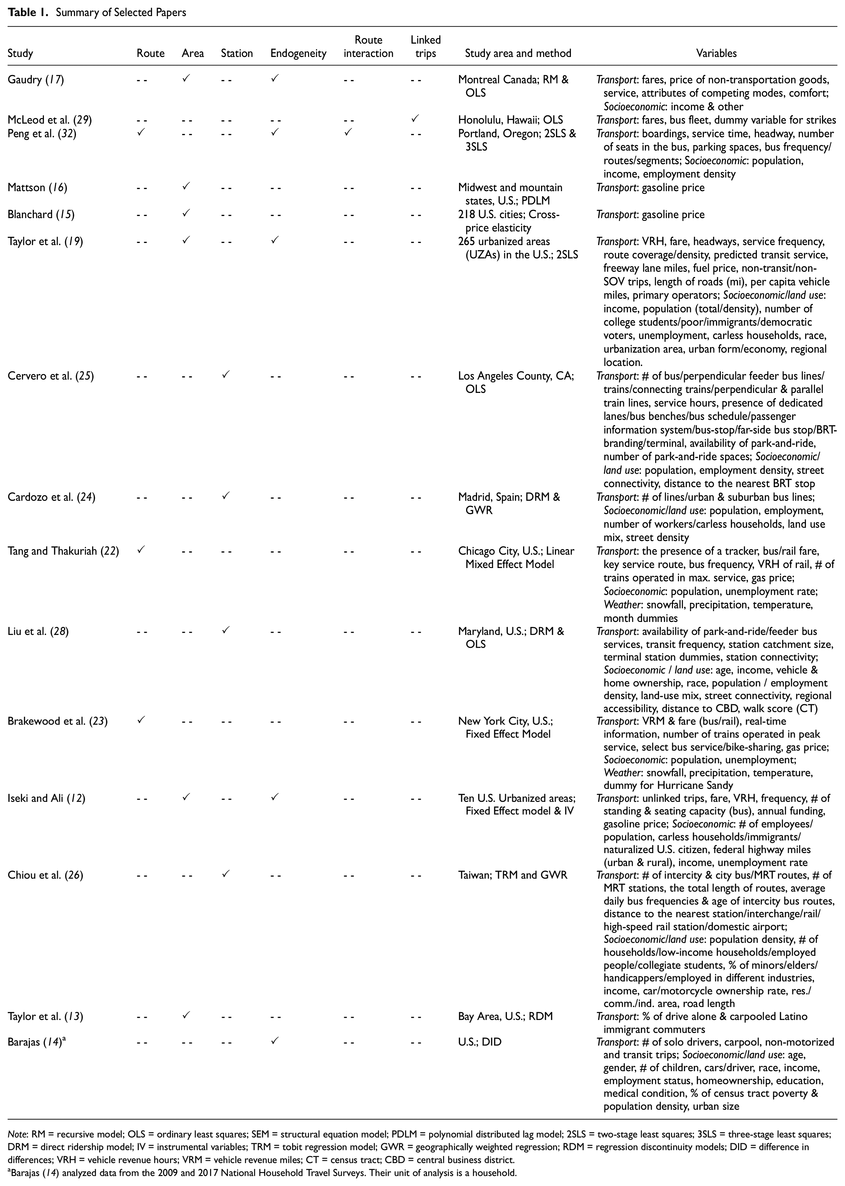
Note: RM = recursive model; OLS = ordinary least squares; SEM = structural equation model; PDLM = polynomial distributed lag model; 2SLS = two-stage least squares; 3SLS = three-stage least squares; DRM = direct ridership model; IV = instrumental variables; TRM = tobit regression model; GWR = geographically weighted regression; RDM = regression discontinuity models; DID = difference in differences; VRH = vehicle revenue hours; VRM = vehicle revenue miles; CT = census tract; CBD = central business district.

Barajas ( 14 ) analyzed data from the 2009 and 2017 National Household Travel Surveys. Their unit of analysis is a household.

Exploratory Analysis

AB 60 and Driving Licenses in Orange County

California has long been the U.S. state with the most immigrants. In 2018, 27 percent of Californians (10.6 million) were foreign-born. Of these, slightly over 20 percent (2.2 million in 2016) were undocumented ( 34 ). Obtaining information about them is difficult. Drivers without a driver’s license cannot obtain vehicle insurance, which likely results in more hit-and-run accidents. After studying the impact on traffic safety of AB 60, Lueders et al. ( 6 ) concluded that AB 60 decreased the rate of hit-and-run accidents, possibly by reducing fears of deportation and vehicle impoundment. As they explain, hit-and-runs tend to delay emergency assistance, increase insurance premiums, and can result in significant out-of-pocket expenses for victims, therefore California (among other states) passed laws such as AB 60.

AB 60 (implemented on January 2, 2015), helped one million undocumented immigrants obtain California driver’s licenses by 2018 ( 5 ). California experienced an increase in the number of driver’s licenses issued by the DMV before the COVID-19 pandemic: between 2008 and 2019, this increase was 15.97%. Orange County experienced a similar trend over the same period, as shown in Figure 1. It shows a gradual increase in the total number of driver’s licenses issued annually by the DMV, with a maximum percentage increase (3.64%) in 2015, the year when AB 60 came into effect.

Figure 1.

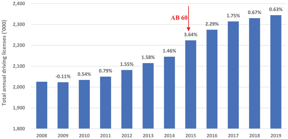
Yearly total driver’s license issued by the Department of Motor Vehicles (DMV) in Orange County, CA.

The California DMV was well aware of the increased demand for driver’s licenses since AB 60, and they were prepared for it: they opened new driving license processing centers, trained new employees, developed regulations for required documents, kept Saturday office hours, and extended office hours on weekdays to meet new customer demand ( 35 ). This allowed the CA DMV to issue 605,000 new driver’s licenses in 2015 ( 35 ). Considering this, we believe that analyzing two years after the inception of AB 60 should be sufficient to capture its short-term impacts.

OCTA Bus Service

OCTA operates five different bus services: 1) major corridors, 2) non-major corridors, 3) community, 4) station link, and 5) express. Table 2 provides a summary of these services. The first two services involve 43 routes (also called local routes), which offer the most frequent service. These routes form a grid on arterial streets and serve the denser parts of Orange County. Figure 2a shows local OCTA routes mainly serving Fullerton, Anaheim, Orange, Garden Grove, Santa Ana, Huntington Beach, Costa Mesa, and Irvine.

Table 2.

OCTA Bus Service Characteristics

Routes	Description	^aService frequency (headway and others)	Boardings (per revenue hour)	^bRidership
Major corridors	22 routes that form a grid on arterial streets	Every 15 to 30 mins (peak), & 30 mins (off-peak) seven days a week.	33	Annual: 32.2 M boardings. Average weekday: 10,000 riders
Non major corridors	21 routes that operate on arterials within the grid created by major corridors	Every 30 to 60 mins (peak), & 35 to 70 mins (off-peak) seven days a week; some operate only on weekdays.	20	Annual: 8.4 M boardings. Average weekday: 2,000 riders
Community	15 routes that connect pockets of transit demand with major destinations and offer local circulation.	Every 45 mins (peak), & 70 mins (off-peak) seven days a week; 5 community routes operate seven days a week; the others operate only on weekdays	15	Annual: 1.1 M boardings. Average weekday: between 350 and 760 riders
Station link	12 routes that serve as rail feeder services designed to connect Metrolink stations to nearby destinations.	Operate during weekday peak hours only, morning peak hour: from station to destinations. evening peak hour: from destinations to stations	16	Annual: 0.3 M boardings. Average weekday: less than 200 riders
Express	10 routes that connect riders over long distance to destinations within and outside of Orange County	Operate on weekdays and only during peak periods; use freeways.	9	Annual: 0.2 M boardings

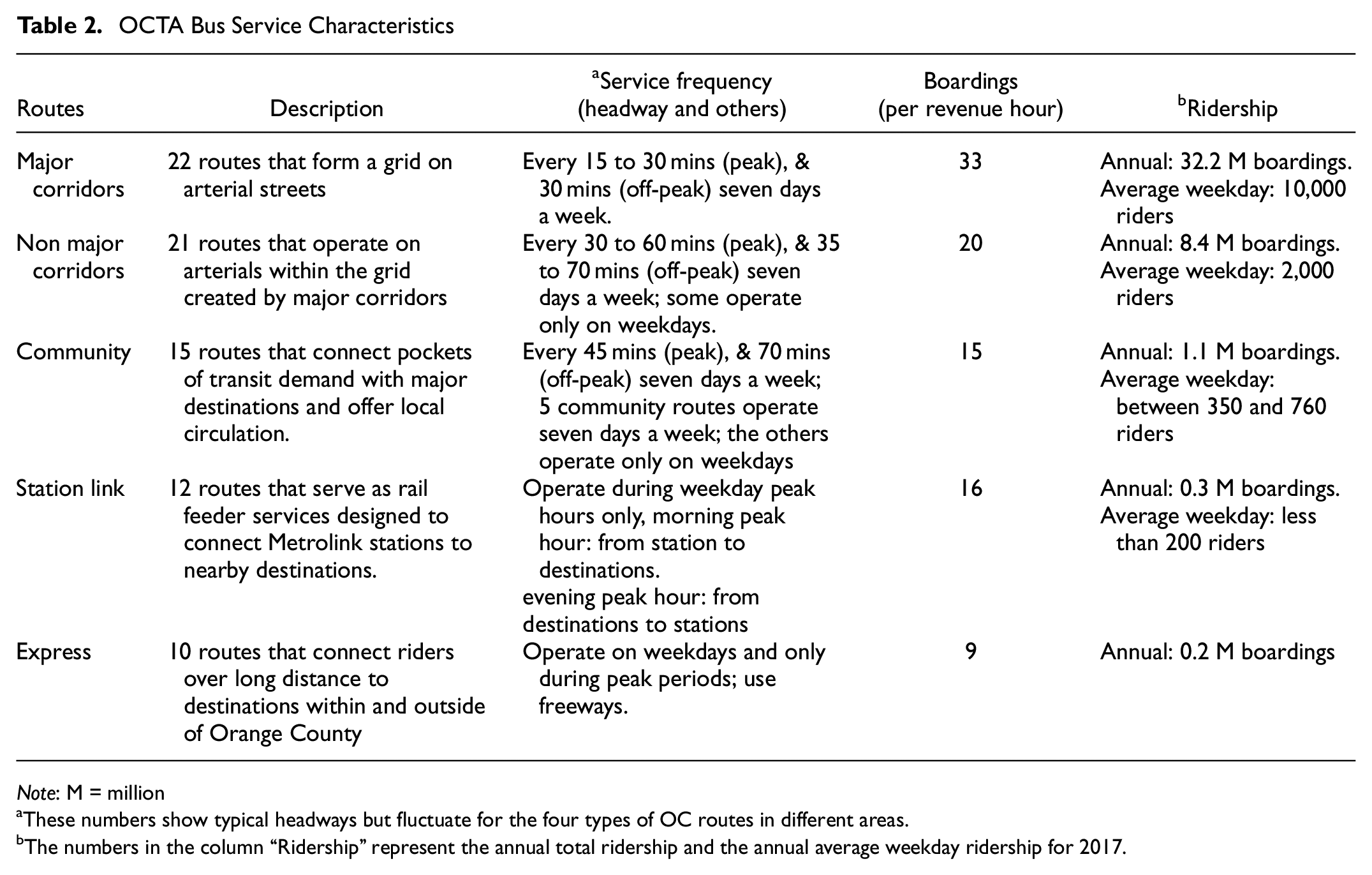
Note: M = million

These numbers show typical headways but fluctuate for the four types of OC routes in different areas.

The numbers in the column “Ridership” represent the annual total ridership and the annual average weekday ridership for 2017.

Figure 2.

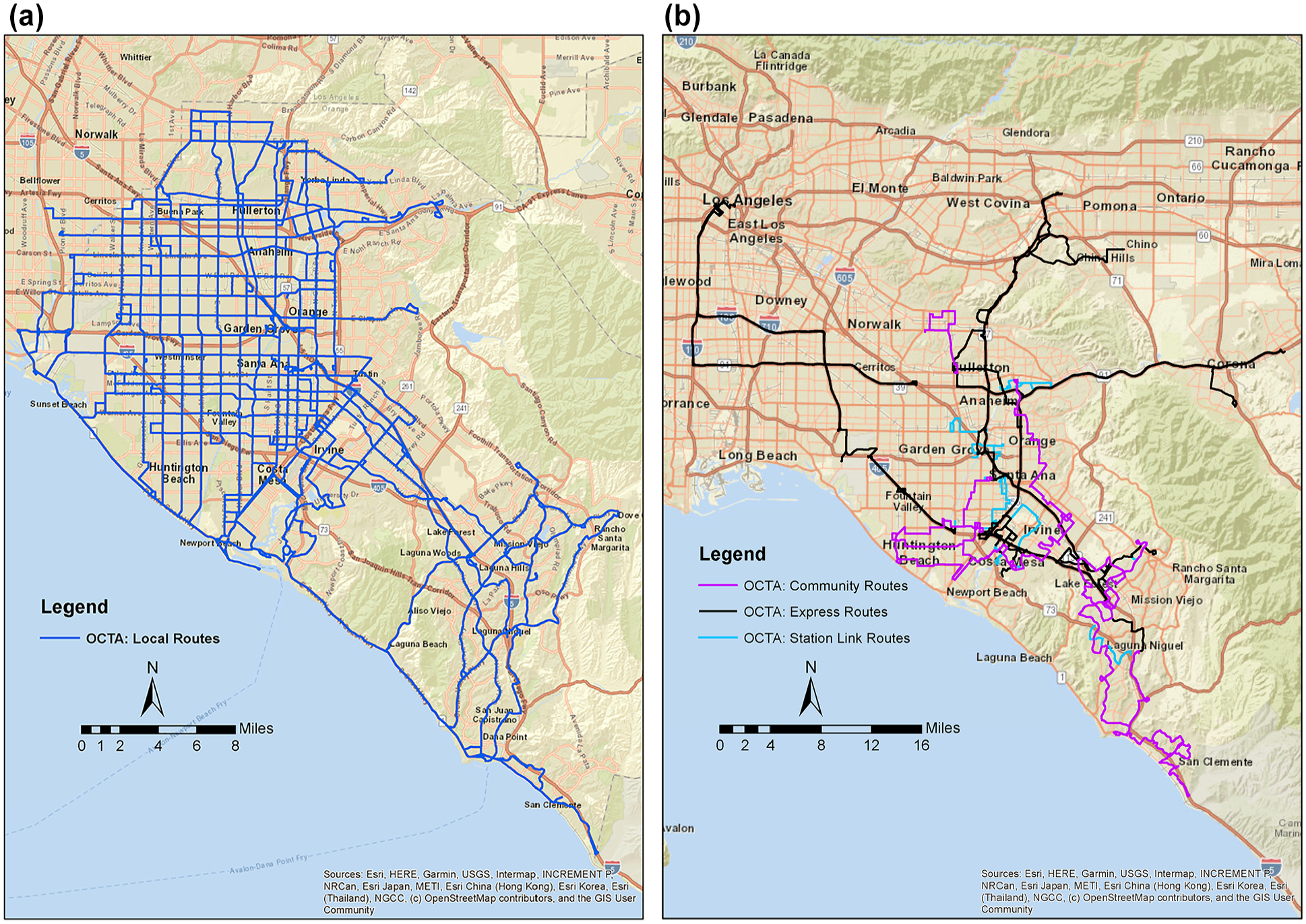
(a) Orange County Transportation Authority (OCTA) local bus routes. (b) OCTA community, station link, and express bus routes.

OCTA also operates low-frequency buses in the community, station links, and express routes (Figure 2b). Community routes link transit pockets and major destinations (Huntington Beach), whereas station links connect Metrolink stations to nearby destinations. Finally, express routes primarily provide long-distance service, such as commuting inside and outside Orange County. In addition to 43 local routes, OCTA operates 15 community routes, 10 express routes, and 12 station link routes for a total of 77 routes.

Bus Ridership Trends in OC: 2014, 2015 and 2016

The dependent variable for our models is the monthly average number of weekday bus boardings on selected OCTA routes from 2014 to 2016. OCTA provided the data. We divided the total weekday boardings of each month by the number of operating days for that month after removing holidays, and averaged them over the routes considered. Figure 3 displays the boarding data for four route types over our study period. It shows a negative linear trend for each year except for station link routes in 2016.

Figure 3.

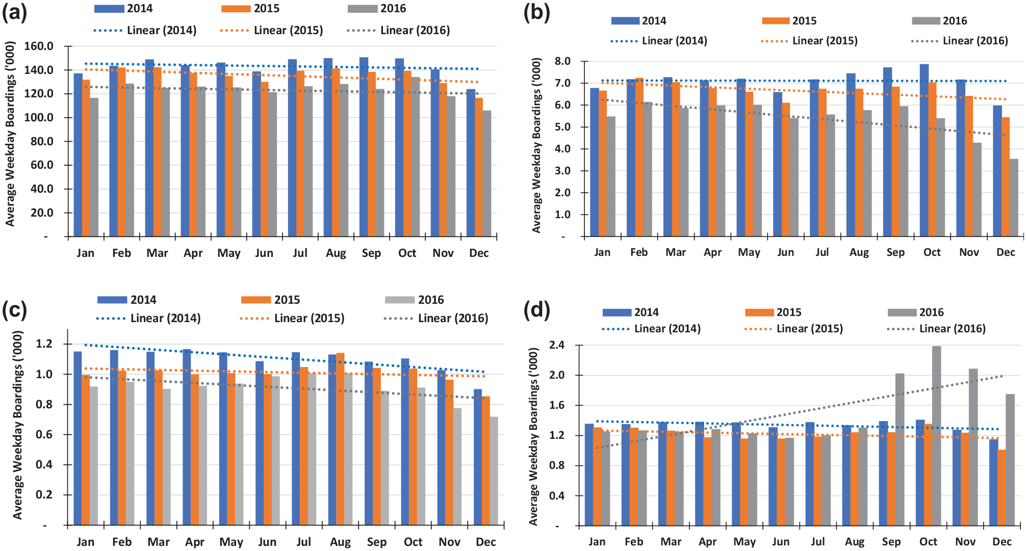
Monthly route-level average weekday boardings for Orange County Transportation Authority (OCTA) (2014-2016). Panel A: Local routes. Panel B: Community routes. Panel C: Express routes. Panel D: Station -link routes.

Although the 2015 and 2016 boardings are consistently below the 2014 boardings for the same month (except for September to December 2016 for station links), drops in boardings depend on route type. Compared with those in 2014, overall boardings in 2015 and 2016 were 5.5% and 14.1% lower on local routes, 6.6% and 23.6% lower on community routes, 8.4% and 17.5% lower on express routes, and 9% and 13.2% lower on station link routes. However, these drops took place during different months.

For local and community routes, boarding declines in 2015 and 2016 appeared to accelerate compared with those in 2014 (as suggested by the linear trends in panels A and B in Figure 3), partly because losses were steeper toward the end of the year. In addition, local routes saw substantial boarding losses in January and June of 2015 and 2016.

For express routes (Panel C), most additional boarding losses occurred during the first five months of 2015 and 2016. The end of 2015 saw the introduction of the OC Bus 360 program (starting in October 2015), which appears to have helped limit boarding losses. As a result, the 2015 boarding trend is nearly horizontal, whereas the 2014 boarding trend is clearly negative. However, in 2016, boardings trended down again.

In contrast, for station link routes (Panel D), the 2015 boarding drop was more evenly spread out during the year. However, boardings in the last four months of 2016 soared because of OCTA’s bus route improvement projects in 2016, which resulted in improved service on some lines.

Data and Models

Dependent Variables

Average weekday route-level boarding data were compiled for each month from January 2014 to December 2016 (36 months). We selected these three years because AB 60 (also known as the Safe and Responsible Drive Act) came into effect on January 2, 2015 ( 36 ), and our goal here is to assess its short-term impact on OCTA bus ridership.

Explanatory Variables

Apart from binary variables that track monthly variations in ridership between 2014 and 2016 (with and without AB 60) and 2015 and 2016 (with AB 60), which allow us to find the ridership difference between 2014 and 2015–2016, explanatory variables for our models can be organized into two groups: 1) internal variables, which are under the control of OCTA, and 2) external variables, which are not.

Our internal variables include route level monthly average bus vehicle revenue hours, and average bus frequency. For our external variables, we considered three rail variables (rail vehicle revenue hours, rail fare, and number of trains operating at peak service) and some monthly sociodemographic and economic variables for different OC cities. The latter include gasoline prices, multifamily home rent and single-family home value by ZIP code, and unemployment rates. We also considered in our models monthly used car values and yearly county-level total number of registered vehicles. Finally, we allowed for monthly variations in 2014 to 2016 to capture the time-varying impacts of AB 60 and other factors. Table 3 provides summary statistics for our variables and indicates their sources.

Table 3.

Summary Statistics

Description	Bus service	Mean	SD	Min.	Max.
Dependent variable
Route level monthly average weekday boarding^a	Local	7.67	1.00	4.81	9.55
	Community	5.91	0.67	4.02	6.92
	Express	4.36	0.76	2.35	5.46
	Station links	4.41	0.78	2.56	5.44
Explanatory variables
Route level:
Monthly average bus vehicle revenue hours^a	Local	7.53	0.70	4.28	8.88
	Community	6.49	0.43	4.18	7.31
	Express	5.23	0.62	3.57	6.34
	Station links	4.97	0.38	3.55	5.77
Monthly average bus frequency^a	Local	0.55	0.40	-0.42	1.37
	Community	0.07	0.20	-0.97	0.62
	Express	0.88	0.68	-0.58	1.75
	Station links	0.86	0.27	0.00	1.21
Monthly total multifamily rent ($)^b	Local	7.54	0.09	7.22	7.80
	Community	7.56	0.09	7.31	7.75
	Express	7.52	0.09	7.20	7.69
	Station links	7.54	0.12	6.77	7.74
Monthly total single-family value ($)^b	Local	13.32	0.17	13.00	13.96
	Community	13.41	0.15	13.03	13.67
	Express	13.32	0.11	12.99	13.49
	Station links	13.29	0.21	12.81	13.66
Monthly total unemployed people^c	Local	8.43	0.54	6.87	9.16
	Community	8.13	0.72	6.62	9.13
	Express	8.65	0.22	8.03	9.21
	Station links	8.64	0.59	6.92	9.46
County level:
Monthly average gasoline price ($/gallon)^d	na	5.78	0.16	5.54	6.07
Monthly average rail vehicle revenue hours^e	na	7.51	0.05	7.38	7.60
Monthly average rail fare ($)^e	na	1.75	0.01	1.73	1.78
Monthly rail scheduled vehicles operating at peak service hours^e	na	5.56	0.12	5.41	5.68

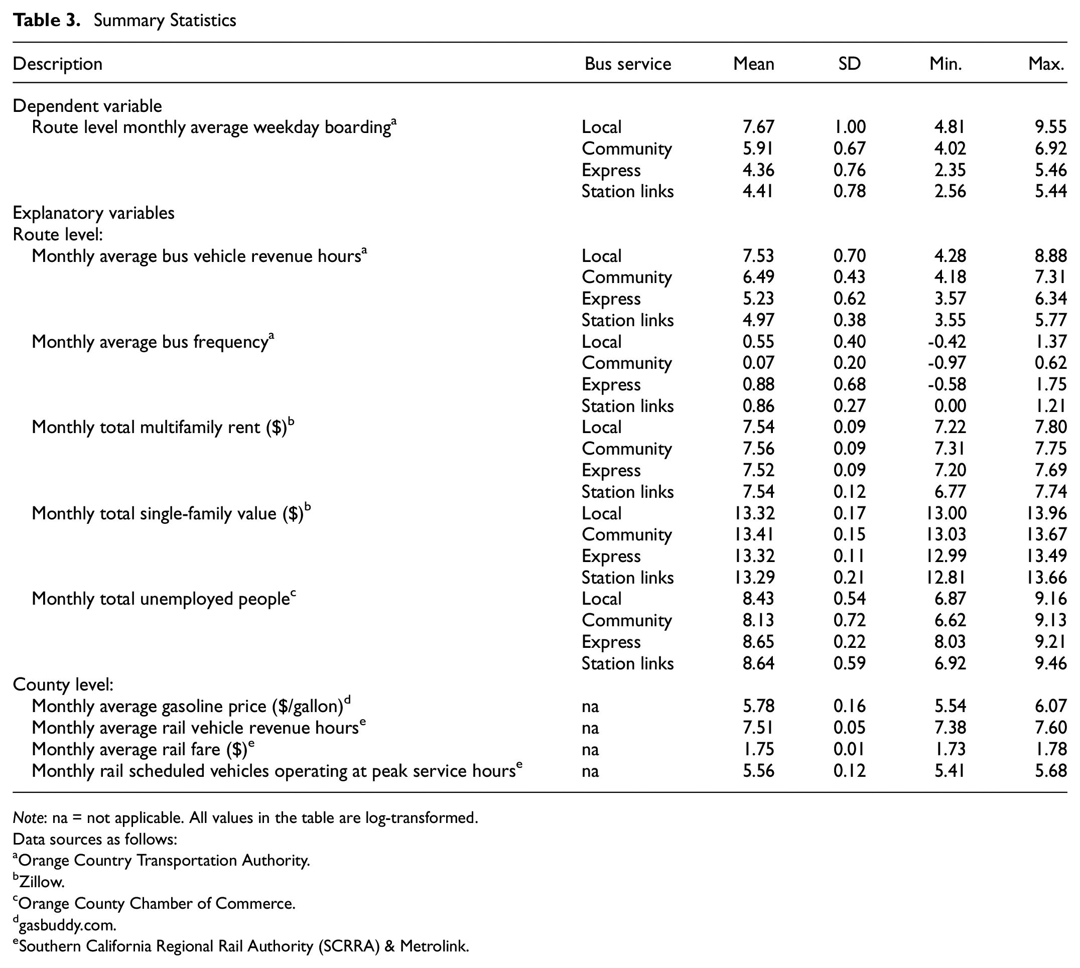
Note: na = not applicable. All values in the table are log-transformed.

Data sources as follows:

Orange Country Transportation Authority.

Zillow.

Orange County Chamber of Commerce.

gasbuddy.com.

Southern California Regional Rail Authority (SCRRA) & Metrolink.

Sociodemographic Variables

We gathered the following sociodemographic variables, which are likely to affect transit ridership: monthly estimates of race, Hispanic people, household structure, educational attainment, median household income, median home value of owner-occupied units, foreign-born populations, and total number of people; all from American Community Surveys 5-year estimates for 2014, 2015, and 2016. We dropped all these variables from our models because of multicollinearity.

Gasoline Price

Several articles have shown that gasoline prices can substantially affect transit ridership (e.g., see [10, 13]). We collected monthly retail gasoline prices for Orange County from Gas Buddy. Figure 4 shows that monthly gasoline prices fluctuated substantially between January 2014 and December 2016, with a maximum of $4.31 per gallon in April 2014 and a minimum of $2.54 in January 2016.

Figure 4.

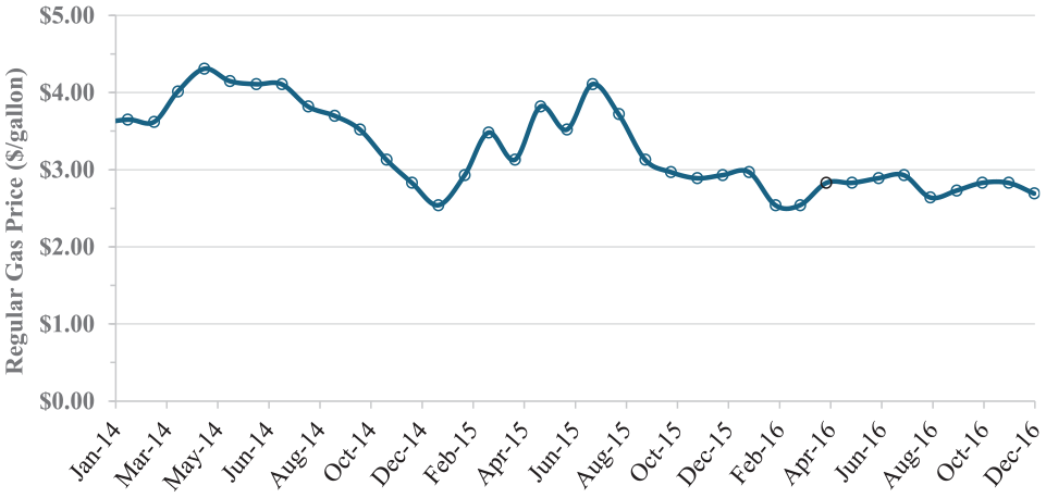
Monthly average gasoline price in Orange County (2014–2016).

Multifamily Rent and Single-Family Home Value

We also collected monthly average multifamily rents and single-family home values by ZIP code from Zillow (https://www.zillow.com/) because several studies ( 37 – 40 ) have shown that multifamily residential units (but not necessarily single-family residences) tend to cluster around transit stops. We added two variables to our models that reflect the rent of multifamily homes and the value of single-family residences on each line, which we calculated using a weighted average based on the number of bus stops in each ZIP code crossed by this line.

Unemployment

Several papers have shown the importance of employment levels on transit ridership (e.g., California Air Resources Board [ 8 ], Manville et al. [ 11 ], Taylor et al. [ 13 ], and Tang and Thakuriah [ 22 ]): transit ridership tends to increase when unemployment is higher, but it decreases with increasing household income because more affluent households can afford and tend to prefer private vehicles. We obtained unemployment data by city (not ZIP code) from the OC Chamber of Commerce. We then used GIS to calculate weighted monthly total unemployment numbers by OCTA line based on the number of bus stops inside each city (essentially the same process as for multifamily housing rents.)

Used Car Cost

We also considered an index of the cost of used cars from the Car Guru website (https://www.cargurus.com/research/price-trends) for 2014 to 2016. This index is weighed by used vehicle registrations and adjusted for age, mileage, condition, and inflation. Since values of this index are provided at unequal intervals, we used interpolation to find the value corresponding to the start of each month. Figure 5 shows an overall decline in used car costs over our study period.

Figure 5.

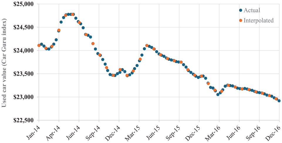
Monthly used car value in the United States (2014–2016).

Number of Registered Motor Vehicles

We also included the total annual number of registered motor vehicles in Orange County in our models to capture the impact of automobile ownership on bus ridership. We collected these data from the DMV.

Rail Variables

Rail variables (Orange County has three lines and 11 stations) were included because rail service interacts with bus ridership (as a complement or a substitute). Systemwide rail service attributes were collected from the Southern California Regional Rail Authority (SCRRA) and Amtrak. We considered rail vehicle revenue hours, rail fare, and the number of trains operating during peak service hours to capture the impact of rail on OCTA bus ridership. Our analysis includes the Orange County and Inland Empire Orange County (IEOC) lines. We collected monthly average passenger fares for Orange County and IEOC lines to model rail fares. However, we had to drop the rail fare variable because of multicollinearity.

Model Specification

Using ordinary least square regression to explain monthly average weekday route-level bus boardings as a function of the explanatory variables described above would yield inconsistent estimates because the assumption that errors are independently and identically distributed with a zero mean does not hold. Indeed, the error terms consist of two unobserved route-level effects: a route-level error and a month-dependent error. Solutions to address this problem include using either a fixed effect or a random effect panel regression model. Although less efficient, a fixed effect model is more suitable because random effect models assume no correlation between the unobserved heterogeneity and the other control variables. Therefore, to explain the monthly changes in OCTA bus ridership, we estimated four route-level fixed-effect panel regression models for the four types of OCTA service routes. For route zϵ{1, …., N} and month tϵ{1, …., T = 36}, our fixed effect model can be written as follows:

\begin{matrix} \ln (B_{zt}) = α_{0} + α_{1} \cdot \ln (VRH B_{zt}) + α_{2} \cdot \ln (B F_{zt}) \\ + α_{3} \cdot \ln (VRH T_{t}) + α_{4} \cdot \ln (R F_{t}) + α_{5} \cdot \ln (MFH R_{zt}) \\ + α_{6} \cdot \ln (SFH V_{zt}) + α_{7} \cdot \ln (U_{zt}) + α_{8} \cdot \ln (G_{t}) \\ + β_{month (t)} + AB 60 (year) \times γ_{month (t)} + δ_{z} + ε_{zt} \end{matrix}

(1)

In Equation 1,

B_zt denotes monthly average weekday boardings for bus route z during month t;

VRHB_zt and $B F_{zt}$ denote respectively the monthly average vehicle revenue hours and frequency for bus route z during month t;

VRHT_t and $R F_{t}$ are the monthly average vehicle revenue hours and fares for OC and IEOC rail lines;

MFHR_zt, $SFH V_{zt}$ and $U_{zt}$ are respectively the route level monthly total multifamily home rent, single family home value and the number of unemployed people;

G_t is the average gasoline price for month t;

β_month(t) is the monthly variation in bus boardings over the study period (2014 to 2016), where month(t) returns the month number in a year (January = 1, …,December = 12);

γ_month(t) is the monthly variation in bus boardings after AB 60, as AB60(2014) = 0, AB60(2015) = 1, and AB60(2016) = 1;

δ_z is a fixed-effect intercept for route z; and

ε_zt is an error term.

Mean differencing removes route-level unobserved effects. It is less efficient, but it yields unbiased and consistent estimates if our models are correctly specified ( 41 ).

We also conducted endogeneity tests to check whether bus vehicle revenue hours are exogenous. For both the Durbin (1954) and Wu–Hausman statistics and Wooldridge’s (1995) robust score test, we found that the test statistics are insignificant, so we are confident that our models do not suffer from an endogeneity problem.

To detect changes in bus ridership after the implementation of AB 60, we compared monthly variations in bus boardings before and after the implementation of AB 60 by comparing $β_{month (t)}$ and $γ_{month (t)}$ , after calculating the corresponding percentage changes by exponentiating, subtracting one, and multiplying by 100% ( 42 ).

Results

Our results were estimated using Stata 17. They are presented in Table 4. Our panel datasets are unbalanced, with N = 77 routes, T = 3 years, 1,432 observations for local routes, 503 for Community routes, 356 for Express routes, and 420 for Station Links. As shown above, we log-transformed our dependent and continuous explanatory variables so the estimated coefficients of continuous variables can be interpreted as elasticities.

Table 4.

Fixed Effect Results by Route Type

Y = Route level monthly average weekday boarding	Local	Community	Express	Station link
Transit attributes
Monthly average route level bus VRH	0.374‡	−0.037	0.082^*	0.189
Monthly average route level bus frequency	0.041	0.051	0.066	−0.453
Monthly average rail VRH	0.086	0.376^*	−0.137	0.098
Yearly total number of trains operating during peak hours	−0.285‡	−0.323‡	−0.030	0.136
Monthly average gas price (cents/gallon)	0.174‡	0.095	0.179	−0.213
Monthly total route level unemployed people	0.413‡	0.362†	0.598^*	0.350^*
Monthly total route level multifamily rent ($)	−0.121^*	−0.492	−0.088	−0.065
Monthly total route level single family value ($)	0.527†	0.228	−0.595	−1.362
Monthly binary variables for 2014–2016
February	0.068‡	0.066†	−0.010	0.014
March	0.068‡	0.067‡	−0.014	0.074
April	0.052‡	0.063	0.077	0.112
May	0.092‡	0.103‡	0.068	0.122
June	0.012	0.002	−0.013	0.057
July	−0.065‡	−0.069†	−0.128^*	−0.046
August	−0.013	−0.063	−0.096	−0.050
September	0.143‡	0.138‡	0.027	0.128
October	0.106‡	0.152‡	0.033	0.071
November	0.140‡	0.127‡	−0.009	0.014
December	−0.005	−0.016	−0.048	−0.106
Monthly binary variables for 2015–2016
January	0.000	−0.020	0.030	0.051
February	0.022^*	0.013	0.071	0.072
March	−0.057‡	−0.045	0.038	0.030
May	−0.047‡	−0.044	0.018	0.003
June	−0.098‡	−0.085†	0.027	−0.029
July	−0.079‡	−0.043	0.038	0.013
August	−0.081‡	0.003	0.108†	0.028
September	−0.081‡	−0.032	0.066	−0.060
October	−0.053‡	−0.053	0.044	0.019
November	−0.109‡	−0.076^*	0.036	0.002
December	−0.079‡	−0.091†	0.034	−0.056
Constant	−4.033	2.690	8.261	18.140
Observations	1432	503	356	420
R ²	0.749	0.572	0.550	0.306
AIC	−3894.5	−955.1	−583.5	−344.3
BIC	−3736.5	−891.8	−544.7	−295.9

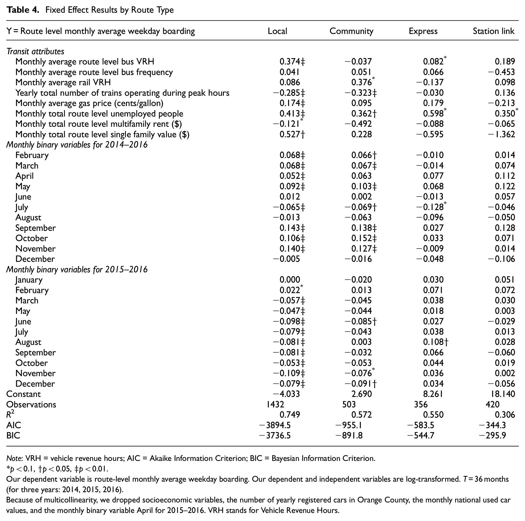
Note: VRH = vehicle revenue hours; AIC = Akaike Information Criterion; BIC = Bayesian Information Criterion.

p < 0.1, †p < 0.05, ‡p < 0.01.

Our dependent variable is route-level monthly average weekday boarding. Our dependent and independent variables are log-transformed. T = 36 months (for three years: 2014, 2015, 2016).

Because of multicollinearity, we dropped socioeconomic variables, the number of yearly registered cars in Orange County, the monthly national used car values, and the monthly binary variable April for 2015–2016. VRH stands for Vehicle Revenue Hours.

To address extensive multicollinearity, we started with a complete set of explanatory variables and eliminated the variable with the highest variance inflation factor (VIF). We iterated until the highest VIF value was around 6.0. We then estimated our models (see Equation 1). The final list of variables for our models excluded exactly one monthly binary variable for each route type (January of 2014–2016, which served as a base), but it corresponded to different months for different route types. Because of multicollinearity, we dropped socioeconomic variables, the number of yearly registered cars in Orange County, the monthly national used car values, and the monthly binary variable April for 2015–2016. The estimated coefficients for our models are presented in Table 4. The results indicate that the signs of the estimated parameters that are statistically significant are as expected.

Internal Factors

Bus vehicle revenue hours are significant only for local and express routes. The results imply that daily boardings on each local route increased by 0.4% and 0.1% for local and express routes, respectively, from a 1% increase in revenue hours of service.

External Factors

Our results suggest that between 2014 and 2016, external factors had a substantial impact on OCTA bus ridership. Among other external factors, train VRH and the maximum number of trains operating at peak hours significantly influenced bus ridership, especially on local and express routes. When the average train VRH increased by 1%, the average monthly weekday bus ridership increased by 0.4% on community routes, which suggests that community routes complemented the OC rail system. Similarly, a 1% increase in trains operating during peak hours reduced weekday bus ridership on local and community boarding by 0.3%. This suggests that local and community bus lines competed with commuter trains in Orange County. Rail VRH and the number of trains operating during peak hours for the other routes are insignificant.

In 2014 to 2016, the impact of changes in gasoline prices on boardings was comparatively large on local and express routes. A 1% increase in gas price increased the average monthly weekday bus ridership by 0.2% on local roads, controlling for other factors. We conjecture that local routes carry a greater percentage of racial minorities and people with a lower annual household income and without private vehicles than express routes do (e.g., see Wu et al. [ 43 ] for differences in socioeconomic characteristics for riders of local and express buses in the Twin Cities). Unfortunately, we do not have access to surveys of transit users for these routes. Therefore, we infer that people with cars are more sensitive to gasoline price increases, so express routes have a higher gas price coefficient than local routes.

Unemployment has a positive coefficient value, highlighting the importance of transit for less affluent groups. The impact of unemployment is significant for all OCTA bus routes. A 1% increase in the unemployment rate increases bus ridership by approximately 0.4% on local routes, community routes and station link routes and 0.6% on express routes.

Coefficients for multifamily rents and single-family home values are also statistically significant. A 1% increase in rent decreases the boardings on local routes by 0.1%. Typically, multifamily rents near transit stops are 10%–20% higher than those farther away. When rent increases, people tend to move away from these locations to cheaper rental areas and replace high rental costs with high transportation costs by not using transit anymore. Orange County is no different ( 44 ).

Moreover, our results show that a 1% increase in single-family home values increases local road boardings by 0.5%. This may seem counterintuitive because wealthier neighborhoods should have more private vehicles and consequently rely less on transit ( 45 ). However, single-family homes located in areas with high quality and dense transit infrastructure benefit from better access, which potentially leads residents to use transit more ( 46 , 47 ). Therefore, we conjecture that this is the case for single-family housing close to Orange County’s local routes.

Monthly Ridership Variations

Monthly ridership variations are partly caused by the rhythm of academic calendars and workers’ holidays, particularly during the summer months and at the end of the year. As a result, ridership tends to be lower in the summer. To better understand how monthly weekday bus boardings changed after the enactment of AB 60 for different route types, we plotted them in Figure 6. It shows that monthly coefficients for local, community, and station link routes decreased for almost all the months in 2015 to 2016 compared with those in 2014. We conjecture that these changes reflect the enactment of AB 60, although we cannot exclude that it was also partly due to the expanding activity of TNCs in Orange County. Nevertheless, like Manville et al. ( 11 ), we note that Uber and Lyft arrived in Southern California only in 2013 and grew significantly only after 2015.

Figure 6.

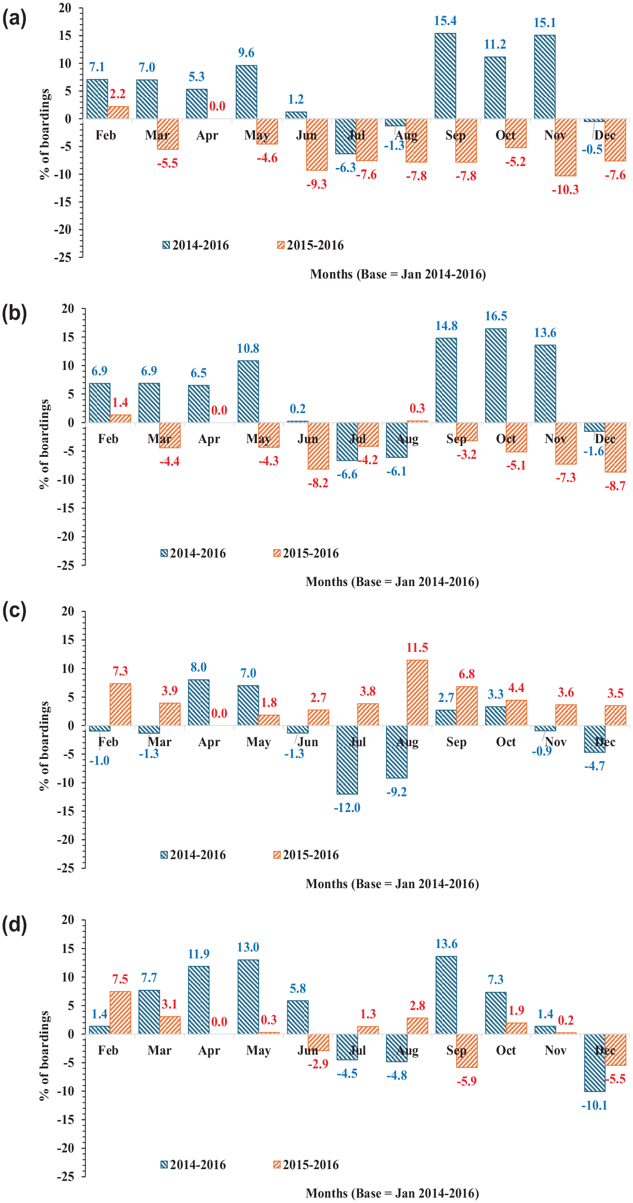
Estimated monthly bus ridership percentage changes (2014–2016 versus 2015–2016). Panel A: Local routes. Panel B: Community routes. Panel C: Express routes. Panel D: Station link routes.

Panel A shows the trend for local routes. The average weekday ridership fell substantially in all the months of 2015 to 2016. The estimated coefficients were statistically significant for all of them except for January. As a result, after averaging monthly coefficients transformed to reflect percentages, bus boardings dropped by 1.7%, 4.6%, 7.7%, and 7.7% in the winter, spring, summer, and fall of 2015 to 2016 compared to 2014.

Similar patterns can be observed for the community routes model (Panel B), where most monthly coefficients are also smaller in 2015 to 2016 than in 2014. A few are statically significant (June, November, and December). For that case, our model estimated that bus boardings dropped by 8.2%, 7.3%, and 8.7% in those three months of 2015 to 2016 compared with 2014.

For express routes, only August of 2015 to 2016 differs significantly from 2014, but its value is higher (Panel D).

In contrast, the monthly coefficients for station link routes were not lower in 2015 to 2016 compared to 2014 for most of the year. Moreover, all the monthly coefficients for these routes for 2015 to 2016 are insignificant.

To explain these patterns, it is helpful to recall that undocumented immigrants in California are overwhelmingly Hispanic, low-income, and foreign-born people ( 48 ). Indeed, census tract data show that local routes serve many areas with relatively high percentages of Hispanic, low-income, and foreign-born people (see Figure 7). Community and station link routes overlap substantially with local routes (see Figure 2). In contrast, express routes serve more affluent areas with fewer foreign-born residents.

Figure 7.

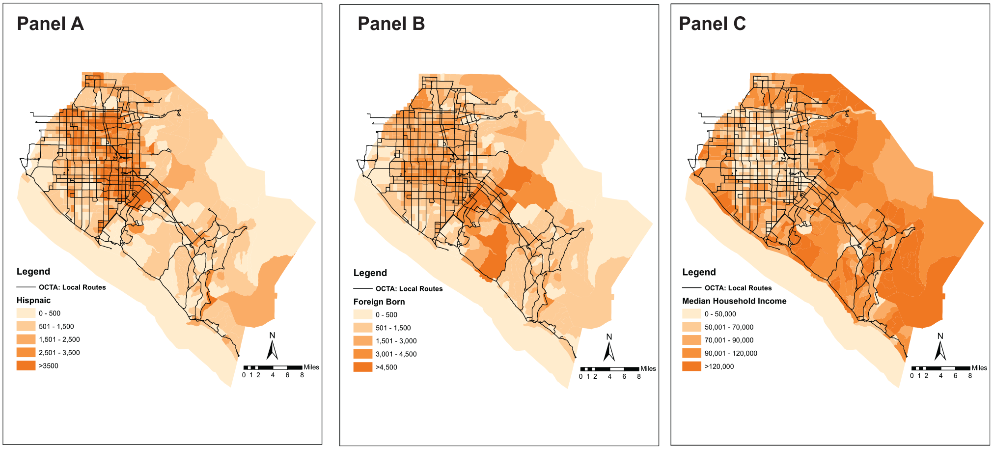
Distributions of Hispanic, foreign-born, and median household income households by Orange County census tract for 2015. Panel A: Hispanic people. Panel B: Foreign born. Panel C: Median household income.

Conclusions

In this study, we evaluated the impact of AB 60 on bus ridership in Orange County. We estimated fixed effect panel regression models for different OCTA routes to explain route-level monthly average weekday bus ridership over a three-year period while controlling for transit vehicle revenue hours, service frequency, and some economic variables. We found time-varying decreases in OCTA bus ridership after AB 60 came into effect. In particular, ridership on local routes, which offer the most frequent service, decreased by 1.7% in the winter, 4.6% in the spring, 7.7% in the summer, and 7.7% in the fall of 2015-2016 compared with the winter, spring, summer, and fall of 2014.

This study fills a gap in the literature by providing some empirical evidence of the unintended consequences on transit of a law designed to give more economic opportunities to undocumented immigrants and to increase road safety. Although we cannot isolate its impacts from those of TNCs, we note that the growth of TNCs in Southern California occurred after 2015 ( 11 ). To the best of our knowledge, this study is also the first to examine bus transit in Orange County, California’s third-most-populous county, and the United States’ sixth-most-populous county. Second only to San Francisco County, it is also the second densest county in California ( 49 ).

The long-term decline in transit ridership in OC is problematic in the context of California’s efforts to rein in VMT to reduce congestion, improve air quality, and achieve its GHG reduction targets. We note, however, that OCTA increased its fares by 50% between 2022 and 2016 ( 10 ). Indeed, OCTA’s average fare in 2015 was the second-highest in Southern California ( 10 ). Moreover, the share of Mexican foreign-born households with no vehicle decreased by 66% between 2000 and 2015 in Southern California ( 10 ). Under assimilation pressures, immigrants tend to behave increasingly like native-born people over time ( 10 ).

Therefore, in addition to improving service (frequency on selected routes) and expanding successful initiatives such as the Bravo! and the OC Bus 360 programs, OCTA may consider offering free transit pass programs targeted at specific groups. These programs could be financed using the insurance model ( 50 ). Even though the impact of free transit pass programs on regaining revamped ridership is mixed, this strategy has been proven to be one of the most effective measures ( 50 – 55 ) available to transit agencies. An example of the potential of these programs is Los Angeles Metro’s GoPass pilot program, which provides free transit passes to K-14 students. It was launched in the fall of 2021, and by the winter of 2023, over 241,000 LA County students had registered and generated over 1.2 million monthly boardings. For other examples of successful free or reduced-fare transit programs, see Chandler ( 55 ).

There are several limitations of this study. First, we could not assess the impact of Uber and Lyft on bus ridership because the California Public Utilities Commission (CPUC) is not releasing detailed Uber and Lyft trip data. Uber and Lyft must report ZIP code-level trip data (including the location, date and time of trips) to the CPUC. When the CPUC indicated that it would release some of these data to the public, Lyft objected, and a judge imposed a stay ( 56 ). We understand that this stay was lifted a few months ago, but the CPUC ignored our freedom of information act request for data. Although we may have overestimated the impacts of AB 60 by not including in our models a variable that reflects the activity of Uber and Lyft in Orange County, we note (see Manville et al. [ 11 ]) that Uber and Lyft only arrived in Southern California in 2013, and their dramatic growth only took place after 2015. Second, we were not able to obtain detailed gasoline price data. Third, it would be interesting to inquire if the California DMV would be willing to provide monthly driver’s license data. However, what matters here is when drivers who obtained their license thanks to AB 60 acquired a motor vehicle and started using it. Addressing these limitations is left for future work, along with an analysis of the impact of AB 60 on rail transit.

Footnotes

Acknowledgements

We are thankful to OCTA for the bus boarding, VRH, frequency, and ZIP code-level multifamily rent data that made this study possible. In particular, we thank Anup Kulkarni, section manager of Regional Modeling and Traffic Operations at OCTA, and Henning Eichler, planning manager of Metrolink. In addition, we thank three anonymous reviewers for their helpful comments, which helped us to substantially improve this paper.

Author Contributions

The authors confirm contribution to the paper as follows: study conception and design: F. Khatun, J.-D. Saphores; data collection: F. Khatun, J.-D. Saphores; analysis and interpretation of results: F. Khatun, J.-D. Saphores; draft manuscript preparation: F. Khatun, J.-D. Saphores. All authors reviewed the results and approved the final version of the manuscript.

Declaration of Conflicting Interests

The author(s) declared no potential conflicts of interest with respect to the research, authorship, and/or publication of this article.

Funding

The author(s) disclosed receipt of the following financial support for the research, authorship, and/or publication of this article: Funding from the Pacific Southwest Region University Transportation Center (PSR UTC) and the state of California (via SB-1).

Data Accessibility Statement

The data analyzed in this paper are available on request.

ORCID iDs

Farzana Khatun

Jean-Daniel Saphores

References

Dickens

Neff

2011 Public Transportation Fact Book. American Public Transportation Association, Washington, D.C., 2011.

Hughes-Cromwick

Dickens

2017 Public Transportation Fact Book. American Public Transportation Association, Washington, D.C., 2017.

OCTA. OC Transit Vision. State of OC Transit. 2017. https://www.octa.net/pdf/State%20of%20OC%20Transit-%20Full%20Report.pdf

Johnson

County Transit Agency Is Evolving to Meet Demand. Opinion Pages of the Orange County Register, August 10. http://www.ocregister.com/2017/08/10/county-transit-agency-is-evolving-to-meet-demand/.

California Department of Motor Vehicles. AB 60 Driver License. https://www.dmv.ca.gov/portal/dmv/detail//index.

Lueders

Hainmueller

Lawrence

Providing Driver’s Licenses to Unauthorized Immigrants in California Improves Traffic Safety. Proceedings of the National Academy of Sciences, Vol. 114, No. 16, 2017, pp. 4111–4116. https://doi.org/10.1073/pnas.1618991114.

California Air Resources Board. California Global Warming Solutions Act of 2006. https://ww2.arb.ca.gov/resources/fact-sheets/ab-32-global-warming-solutions-act-2006.

California Air Resources Board. The Sustainable Communities and Climate Protection Act of 2008. https://ww2.arb.ca.gov/our-work/programs/sustainable-communities-climate-protection-program.

Taylor

B. D.

Fink

C. N. Y.

Explaining Transit Ridership: What Has the Evidence Shown?

Transportation Letters, Vol. 5, No. 1, 2013, pp. 15–26. https://doi.org/10.1179/1942786712Z.0000000003.

10.

Manville

Taylor

B. D.

Blumenberg

Falling Transit Ridership: California and Southern California. ITS, UCLA, CA, 2018, pp. 1–83.

11.

Manville

Taylor

B. D.

Blumenberg

Schouten

Vehicle Access and Falling Transit Ridership: Evidence from Southern California. Transportation, Vol. 50, No. 1, 2023, pp. 303–329. https://doi.org/10.1007/s11116-021-10245-w.

12.

Iseki

Ali

Fixed-Effects Panel Data Analysis of Gasoline Prices, Fare, Service Supply, and Service Frequency on Transit Ridership in 10 U.S. Urbanized Areas. Transportation Research Record: Journal of the Transportation Research Board, 2015. 2537: 71–80.

13.

Taylor

B. D.

Blumenberg

Wasserman

J. L.

Garrett

Schouten

King

Paul

Ruvolo

Transit Blues in the Golden State: Analyzing Recent California Ridership Trends. University of California Institute of Transportation Studies, 2020. https://doi.org/10.17610/T67W2Z.

14.

Barajas

J. M.

The Effects of Driver Licensing Laws on Immigrant Travel. Transport Policy, Vol. 105, 2021, pp. 22–34. https://doi.org/10.1016/j.tranpol.2021.02.010.

15.

Blanchard

The Impact of Rising Gasoline Prices on US Public Transit Ridership. Duke University, Durham, NC, 2009.

16.

Mattson

Effects of Rising Gas Prices on Bus Ridership for Small Urban and Rural Transit Systems. Upper Great Plains Transportation Institute, North Dakota State University, Fargo, 2008.

17.

Gaudry

An Aggregate Time-Series Analysis of Urban Transit Demand: The Montreal Case. Transportation Research, Vol. 9, No. 4, 1975, pp. 249–258. https://doi.org/10.1016/0041-1647(75)90066-0.

18.

Taylor

B. D.

Miller

Iseki

Fink

Analyzing the Determinants of Transit Ridership Using a Two-Stage Least Squares Regression on a National Sample of Urbanized Areas. University of California Transportation Center, 2003.

19.

Taylor

B. D.

Miller

Iseki

Fink

Nature and/or Nurture? Analyzing the Determinants of Transit Ridership Across US Urbanized Areas. Transportation Research Part A: Policy and Practice, Vol. 43, No. 1, 2009, pp. 60–77. https://doi.org/10.1016/j.tra.2008.06.007.

20.

Guo

Wilson

N. H. M.

Rahbee

Impact of Weather on Transit Ridership in Chicago, Illinois. Transportation Research Record: Journal of the Transportation Research Board, 2007. 2034: 3–10.

21.

Witte

A. D.

Macharis

Lannoy

Polain

Steenberghen

Van de Walle

The Impact of “Free” Public Transport: The Case of Brussels. Transportation Research Part A: Policy and Practice, Vol. 40, No. 8, 2006, pp. 671–689. https://doi.org/10.1016/j.tra.2005.12.008.

22.

Tang

Thakuriah

Ridership Effects of Real-Time Bus Information System: A Case Study in the City of Chicago. Transportation Research Part C: Emerging Technologies, Vol. 22, 2012, pp. 146–161. https://doi.org/10.1016/j.trc.2012.01.001.

23.

Brakewood

Macfarlane

G. S.

Watkins

The Impact of Real-Time Information on Bus Ridership in New York City. Transportation Research Part C: Emerging Technologies, Vol. 53, 2015, pp. 59–75. https://doi.org/10.1016/j.trc.2015.01.021.

24.

Cardozo

O. D.

García-Palomares

J. C.

Gutiérrez

Application of Geographically Weighted Regression to the Direct Forecasting of Transit Ridership at Station-Level. Applied Geography, Vol. 34, 2012, pp. 548–558. https://doi.org/10.1016/j.apgeog.2012.01.005.

25.

Cervero

Murakami

Miller

M. A.

Direct Ridership Model of Bus Rapid Transit in Los Angeles County. Institute of Transportation Studies at UC Berkeley, 2009.

26.

Chiou

Y.-C.

Jou

R.-C.

Yang

C.-H.

Factors Affecting Public Transportation Usage Rate: Geographically Weighted Regression. Transportation Research Part A: Policy and Practice, Vol. 78, 2015, pp. 161–177. https://doi.org/10.1016/j.tra.2015.05.016.

27.

Gutiérrez

Cardozo

O. D.

García-Palomares

J. C.

Transit Ridership Forecasting at Station Level: An Approach Based on Distance-Decay Weighted Regression. Journal of Transport Geography, Vol. 19, No. 6, 2011, pp. 1081–1092. https://doi.org/10.1016/j.jtrangeo.2011.05.004.

28.

Liu

Erdogan

Ducca

F. W.

How to Increase Rail Ridership in Maryland? Direct Ridership Models (DRM) for Policy Guidance. Presented at the 2014 TRB Annual Meeting, 2014. https://www.researchgate.net/publication/263809618

29.

McLeod

M. S.

Flannelly

K. J.

Flannelly

Behnke

R. W.

Multivariate Time-Series Model of Transit Ridership Based on Historical, Aggregate Data: The Past, Present and Future of Honolulu. Transportation Research Record: Journal of the Transportation Research Board, 1991. 1297: 76–84.

30.

Taylor

B. D.

Fink

C. N. Y.

The Factors Influencing Transit Ridership: A Review and Analysis of the Ridership Literature. University of California Transportation Center, 2003.

31.

Alperovich

Michael

A. K.

Keith

M. G.

An Econometric Model of Bus Transit Demand and Supply. Urban Institute, Washington D. C., 1977.

32.

Peng

Z.-R.

Dueker

K. J.

Strathman

Hopper

A Simultaneous Route-Level Transit Patronage Model: Demand, Supply, and Inter-Route Relationship. Transportation, Vol. 24, 1997, pp. 159–181.

33.

Khatun

Saphores

J.-D.

What Explains Recent Trends in Orange County Transportation Authority Bus Ridership? Publication PSR-18-15. PSR UTC, CA, 2018, pp. 1–30.

34.

American Immigration Council. Fact Sheet: Immigrants in California. https://www.americanimmigrationcouncil.org/research/immigrants-in-california.

35.

AB 60: 605,000 Driver Licenses Issued in First Year. CA DMV, 2016. https://www.dmv.ca.gov/portal/news-and-media/dmv-surpasses-1-million-driver-licenses-under-ab-60/

36.

ACLU Southern California. The Safe and Responsible Drive Act (AB 60). https://www.aclusocal.org/en/know-your-rights/your-rights-ab-60-drivers-license.

37.

Zhong

Rail Transit Investment and Property Values: An Old Tale Retold. Transport Policy, Vol. 51, 2016, pp. 33–48. https://doi.org/10.1016/j.tranpol.2016.05.007.

38.

Wegmann

Death to Single-Family Zoning…and New Life to the Missing Middle. Journal of the American Planning Association, Vol. 86, No. 1, 2020, pp. 113–119. https://doi.org/10.1080/01944363.2019.1651217.

39.

Singer

M. E.

How Affordable Are Accessible Locations? Neighborhood Affordability in U.S. Urban Areas with Intra-Urban Rail Service. Cities, Vol. 116, 2021, p. 103295. https://doi.org/10.1016/j.cities.2021.103295.

40.

Duncan

Comparing Rail Transit Capitalization Benefits for Single-Family and Condominium Units in San Diego, California. Transportation Research Record: Journal of the Transportation Research Board, 2008. 2067: 120–130.

41.

Wooldridge

J. M.

Econometric Analysis of Cross Section and Panel Data. MIT Press, Cambridge, 2010.

42.

How Do I Interpret a Regression Model When Some Variables Are Log Transformed? UCLA Advanced Research Computing: Statistical Methods and Data Analytics. https://stats.oarc.ucla.edu/other/mult-pkg/faq/general/faqhow-do-i-interpret-a-regression-model-when-some-variables-are-log-transformed/.

43.

Cao

Huting

Using Three-Factor Theory to Identify Improvement Priorities for Express and Local Bus Services: An Application of Regression with Dummy Variables in the Twin Cities. Transportation Research Part A: Policy and Practice, Vol. 113, 2018, pp. 184–196. https://doi.org/10.1016/j.tra.2018.04.003.

44.

Housing and Transportation. California Department of Housing and Community Development. https://www.hcd.ca.gov/policy-and-research/intersectional-policy-work/housing-and-transportation.

45.

Mattson

Relationships Between Density, Transit, and Household Expenditures in Small Urban Areas. Transportation Research Interdisciplinary Perspectives, Vol. 8, 2020, p. 100260.

46.

Economic Impact of Public Transportation Investment. American Public Transportation Association (APTA), Washington, D.C., 2020.

47.

Boarnet

Bostic

Williams

Affordable Housing in Transit-Oriented Developments: Impacts on Driving and Policy Approaches. Publication CA17-2983. University of California, Davis, p. 37.

48.

Migration Policy Institute. Profile of the Unauthorized Population - CA. migrationpolicy.org. https://www.migrationpolicy.org/data/unauthorized-immigrant-population/state/CA. Accessed June 14, 2024.

49.

Overview of the United States. Statistical Atlas. https://statisticalatlas.com/United-States/Overview.

50.

Saphores

J.-D.

Shah

Khatun

A Review of Reduced and Free Transit Fare Programs in California. University of California Institute of Transportation Studies, 2020. https://doi.org/10.7922/G2XP735Q.

51.

McDonald

Librera

Deakin

Free Transit for Low-Income Youth: Experience in San Francisco Bay Area, California. Transportation Research Record: Journal of the Transportation Research Board, 2004. 1887: 153–160.

52.

Nuworsoo

C. K.

Deep Discount Group Pass Programs as Instruments for Increasing Transit Revenue and Ridership. Institute of Transportation Studies at UC Berkeley, 2004.

53.

Wexler

Ryan

Das

Fan

Free Transit Passes and School Attendance Among High School Students. Transportation Research Record: Journal of the Transportation Research Board, 2021. 2675: 135–147.

54.

Morgan-Roselló

R. G.

A Fare Approach to Attracting Transit Ridership After COVID-19. Doctoral dissertation. Massachusetts Institute of Technology, Cambridge, 2021.

55.

Chandler

L.A. Metro Transit Ridership Up 10 Percent, Sets Post-Pandemic Record. Metro. https://www.metro.net/about/la-metro-transit-ridership-up-10-percent-sets-post-pandemic-record/.

56.

Order Granting Stay of Decision 23-12-015 (Before the Public Utilities Commission of the State of California). February21, 2024.

Driver’s Licenses for Undocumented Immigrants and Bus Ridership in Orange County,California

Abstract

Keywords

Literature Review

Exploratory Analysis

AB 60 and Driving Licenses in Orange County

OCTA Bus Service

Bus Ridership Trends in OC: 2014, 2015 and 2016

Data and Models

Dependent Variables

Explanatory Variables

Sociodemographic Variables

Gasoline Price

Multifamily Rent and Single-Family Home Value

Unemployment

Used Car Cost

Number of Registered Motor Vehicles

Rail Variables

Model Specification

Results

Internal Factors

External Factors

Monthly Ridership Variations

Conclusions

Footnotes

Acknowledgements

Author Contributions

Declaration of Conflicting Interests

Funding

Data Accessibility Statement

ORCID iDs

References