Sage Journals: Discover world-class research

Abstract

Quantifying pedestrian exposure for intersections is important for developing pedestrian-centric strategies. Exposure is typically expressed as the annual-average daily pedestrian traffic (AADPT). AADPT can be directly calculated when continuous counts (CCs) are available. However, CCs are rarely available for all intersections, requiring estimation methods. This work explores the steps involved in expanding pedestrian short-term counts (STCs) to AADPT using factor groups. Day-of-week-of-month expansion factors were used to expand 8-h STCs. The first step consists of grouping sites with similar pedestrian activity patterns (factor groups). Five factor groups were identified, and three pedestrian temporal pattern indicators were proposed to characterize them. The thresholds of these indicators for grouping sites with CCs are available in this work. The second step involves the challenge of associating sites where only STCs are available (unknown traffic patterns) with a particular factor group. Multinomial logistic regression (MLR) was developed to link factor groups to land use, socioeconomic, and operational attributes. Explanatory variables that represent commercial and industrial areas and the number of schools and transit stops were found to be significant. Simpler methods were also introduced to identify factor groups strongly affected by schools. The last step assesses the expansion of STCs to AADPT using the proposed approaches. The results showed improved performance when compared with averaging expansion factors across all sites. It was also demonstrated that, in certain cases, simple approaches that rely exclusively on the identification of sites that are highly affected by schools present similar performance to more complex approaches, such as MLR.

Keywords

pedestrian volume expansion factors factor groups short-term counts multinomial logistic regression

Quantifying pedestrian activity at intersections is crucial for developing pedestrian-centric strategies. Decision-making processes in planning, safety, and traffic operations, with a focus on pedestrians, require a comprehensive understanding of pedestrian exposure in the road network. For example, the development of safety performance functions to establish rankings of critical intersections or the selection of intersections for the deployment of exclusive signal phases for pedestrians are applications that rely on pedestrian volume as inputs ( 1 – 3 ).

Objectives

Short-term counts (STCs) and continuous counts (CCs) are the two typical sources of pedestrian volume data for jurisdictions. STCs are collected for specific hours over 1 or a few days, with durations that vary from 1 to 24 h. They are commonly gathered for urban planning or traffic signal timing purposes. CCs provide long-term information (i.e., months or years) and are useful for the identification of hourly, daily, and monthly patterns of the pedestrian volume across different sites.

STCs collected for the purpose of intersection capacity analysis or traffic signal warrant analysis are usually collected for 4, 8, or 12 h of a typical weekday. This paper uses 1-day STCs collected for 8 h, covering the a.m. peak period (7 to 9 a.m.), midday period (11 a.m. to 2 p.m.), and p.m. peak period (3 to 6 p.m.). This represents the typical framework for data collection for signal timing purposes, which is likely the most common and accessible source of pedestrian data available for jurisdictions.

Pedestrian exposure at intersections is usually expressed as the annual-average daily pedestrian traffic (AADPT). AADPT can be directly calculated at sites with available CCs. However, since CCs are rarely available for all sites in a jurisdiction ( 4 ), methods for estimating AADPT are necessary. When CCs are available for a reasonable number of sites (this number is presented in a later section) and STCs are available for the remaining sites, then AADPT can be estimated with the use of expansion factors calculated from sites with CCs. There are studies available in the literature that investigated different durations and periods of collection of STCs and provide recommendations for optimizing their expansion to AADPT ( 5 – 8 ).

The temporal pattern of pedestrian volume at an intersection, whether considered on an hourly, daily, or monthly basis, is influenced by factors such as land use, socioeconomic conditions, and operational features in its vicinity ( 9 , 10 ). Therefore, the expansion factor method requires that CC sites be classified into factor groups such that the sites in each group have similar pedestrian activity patterns and the patterns across the groups are different. Expansion factors are developed for each factor group and applied to STCs. For reducing error when expanding STCs, Nordback et al. ( 11 ) suggested that at least five CC stations be available for each factor group.

One challenge of the expansion factor method lies in identifying factor groups. Three approaches are commonly found in the literature. The first is the visual classification of sites based on their temporal patterns ( 9 , 12 ). The second is the use of machine learning techniques to group similar temporal patterns ( 10 , 13 ). The third—and most common—is the development of temporal indicators based on the CCs available ( 6 , 7 , 11 , 14 , 15 ). For instance, Miranda-Moreno et al. ( 14 ) proposed two indicators to classify bicycle traffic patterns: WWI, the relative index of weekend and weekday volume; and AMI, the relative index of the a.m. peak (7 to 9 a.m.) and the midday period (11 a.m. to 1 p.m.) volume. Using different thresholds for these indicators, the authors categorized sites as utilitarian, mixed-utilitarian, mixed-recreational, and recreational. Although initially developed for bicycle volume patterns, studies on pedestrians have also used the same indicators. Johnstone et al. ( 7 ) exclusively applied AMI, while Nordback et al. ( 11 ) solely utilized WWI.

The primary limitation of existing temporal indicators to characterize different factor groups lies in their emphasis on measuring intraday and weekday-to-weekend variations without accounting for seasonal fluctuations throughout the year. For instance, consider two hypothetical sites where the pedestrian traffic at one is influenced by the proximity of a high school, while the pedestrian traffic at the other is primarily determined by the presence of a manufacturing plant. It is expected that the AMIs and WWIs of both sites will be similar because of the higher pedestrian volume during the morning peak and on weekdays, as opposed to the midday period and weekends, respectively. However, it is likely that the site associated with the high school will experience reduced volume during school holidays, while the one linked to the manufacturing plant will likely maintain a relatively steady pattern throughout the year. Consequently, the expansion factors for both sites differ, requiring their classification into distinct factor groups. This distinction would not occur if only AMI and WWI were used.

The second significant challenge in employing the expansion factor method is how to select the factor group from which expansion factors should be used for an STC site. Given the absence of CCs, the long-term temporal pattern of pedestrian activity of the STC site is unknown. A common approach used in previous studies is the application of either AMI, WWI, or both, using the information from the STCs to associate the sites with a factor group. However, this approach has its limitations: (I) in cases where only brief STCs are available (e.g., for a few hours), AMI estimation is not feasible; (II) when only 1-day STCs are accessible, WWI cannot be estimated; and (III) as discussed above, these indicators do not account for seasonal effects. To overcome these limitations, models that do not rely on empirical traffic data and are instead based on land-use, socioeconomic, and operational attributes have been applied to associate STC sites with factor groups.

Medury et al. ( 9 ) and Humagain and Singleton ( 10 ) are two examples of pedestrian-centric studies that developed models to associate STC sites with factor groups. Methodologically, both studies are similar: they begin by identifying factor groups using sites with CCs. Then, they associate each factor group with land-use (e.g., commercial use and the presence of schools), socioeconomic (e.g., population density and household size), and operational (e.g., intersection density) attributes using multinomial logistic regressions (MLR). Finally, they assess the accuracy of the expansion of STCs to long-term pedestrian volumes. The results from Medury et al. ( 9 ) demonstrate benefits that range from a 0.8% to a 7.4% absolute reduction in the mean absolute percent error (MAPE) when employing the MLR approach compared with a simple method using a single expansion factor averaged from all sites.

These two studies have made valuable contributions to the field. However, they may have certain limitations and do not encompass all possible configurations of STCs. This creates an opportunity for further research on the topic. For instance, neither study used the actual AADPT as their target measure. Medury et al. ( 9 ) employed data from June to September, while Humagain and Singleton ( 10 ) relied on pedestrian volume data extrapolated from traffic signal push buttons ( 16 ). Furthermore, both studies focused on expanding hourly volume to weekly volume, with Humagain and Singleton ( 10 ) also developing month-of-year factors. Consequently, there is uncertainty about the magnitude of error associated with expanding commonly available 8-h STCs to estimate AADPT.

Given the existing limitations and literature gap on the identification of factor groups using temporal indicators and on the magnitude of error associated with expanding 8-h STCs to AADPT, the objectives of this work are to fill these knowledge gaps by (I) proposing and applying pedestrian volume temporal indicators that capture seasonal trends to identify factor groups, (II) determining the thresholds of these indicators for the identification of factor groups, (III) developing multinomial logit regression models to link STC sites with a particular factor group, (IV) quantifying the error associated with the expansion of 8-h STCs to AADPT, and (V) evaluating the implementation of simpler models and their trade-off in complexity versus performance. Objective (V) is a practical investigation that may help jurisdictions with their decision-making, based on the level of information they have available.

Work Structure

The structure of this work follows the steps a practitioner would take to apply the expansion factor method to STCs using factor groups (Figure 1). The first step involves identifying factor groups from sites with CCs and calculating expansion factors for each set of factor groups. In the second step, factor groups are modeled as a function of land-use, socioeconomic, and transportation attributes, enabling the association of STC sites (i.e., sites with unknown traffic patterns) with factor groups. The final step encompasses the expansion of STCs to AADPT by applying the expansion factors and models obtained from steps 1 and 2, respectively.

Figure 1.

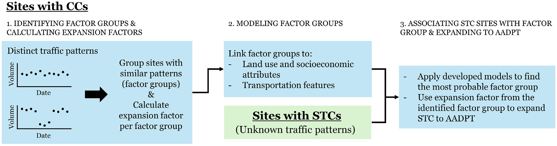
Proposed framework.

Additionally, the two subsequent sections outline the data sources and present an assessment of types of expansion factors. These sections provide complementary information required for the implementation of the core method. The work concludes with a section presenting conclusions and practical recommendations.

Data Sources

This work uses data from the Region of Waterloo, Ontario, Canada. The Region of Waterloo is formed by three cities (Cambridge, Kitchener, and Waterloo) and four townships. It has an area of 1,369 km² and a population of about 650,000. The region shares a similar latitude with the City of Toronto, resulting in four distinct seasons, including cold winters (average daytime high temperatures ≤ 0°C [32°F] for December through February) and hot summers (average daytime high temperatures ≥ 24°C [75°F] for June through August) ( 17 ). The seasonality of the weather may have a significant impact on pedestrian traffic patterns.

Pedestrian volume data were collected from camera-based CC stations located at 78 signalized intersections in the three cities that compose the region. These stations were primarily installed for signal timing and coordination purposes; they were placed them in urban areas. Consequently, this dataset may underrepresent sites with predominantly recreational pedestrian trip activity. The CC stations record motorized vehicle, bicyclist, and pedestrian counts for each turning movement and crosswalk at 1-min intervals on a continuous (24/7) basis. Only sites that met the following two data quality/quantity criteria were included in the study:

The CC station was considered to be collecting data properly on a given day if (I) at least 72 (out of 96) 15-min count intervals had at least one motorized vehicle counted on any approach and (II) the total daily pedestrian volume was > 0.

The CC station was operational for the 12-month period from May 1, 2022, to April 31, 2023, and had properly collected data on at least 95% (345) of these days.

In addition, a filter was applied to the pedestrian counts each month for each site to remove days that represented outliers: daily (24-h) pedestrian volumes that were outside the limits of either (I) the third quartile plus 1.5 times the interquartile range or (II) the first quartile minus 1.5 times the interquartile range. This filtering criterion resulted in the removal of 1.1% of days across the 78 sites.

In the subsequent sections of this work, results will be presented based on 8-h STCs obtained from all available days throughout the year (i.e., days when the CC station was operating properly and that were not removed by the filtering criterion) as well as from a subset of days referred to as “candidate” days. It is a common practice for jurisdictions to collect STCs, particularly for signal timing purposes, on days characterized as having typical traffic volumes. In this work, the candidate days specifically refer to non-holiday Tuesdays, Wednesdays, and Thursdays in the months of April, May, June, September, October, and November. These months are chosen to exclude periods of inclement weather and school holidays.

Assessing Types of Expansion Factors

Three types of expansion factors are commonly employed in practice. The first and simplest type involves using 7 day-of-week (DOW) and 12 month-of-year (MOY) factors, for a total of 19 factors. The second requires estimating a factor for every day-of-week-of-month (DOWOM), for a total of 84. The third and most complex approach utilizes factors for each individual day-of-year (DOY), often referred to as the disaggregated method (for a total of 365 factors). The DOY method allows for the capture of volume oscillations on a daily basis, enabling the discernment of atypical days influenced by factors such as inclement weather or special events like concerts or sports events. Consequently, it has demonstrated better performance when compared with the DOW & MOY and DOWOM approaches ( 6 , 18 ). Despite its advantages, its practical application poses challenges, including that (I) CC stations must operate properly during all days of the year, (II) STCs must be available in the same years as the long-term counts, and (III) identifying factor groups using this level of disaggregation still presents uncertainties. Given these practical difficulties, this work exclusively considered the DOW & MOY and DOWOM factors.

The following procedure was employed to determine whether the DOW & MOY or DOWOM factors give superior performance. The initial step involved calculating the true AADPT for each site using Equation 1. Note that this expression can be used even when daily counts are not available for all days in the year. The only requirement is that there is at least one valid daily count for each day of the week in each month. All 78 sites used in this study met that requirement. Subsequently, factors to expand 8-h STCs to AADPT were computed for each site (Equation 2 illustrates the formulation of the DOWOM factor). Given the availability of CCs for all sites, multiple STCs can be considered, and the AADPT for each is estimated using Equation 3. Finally, the absolute percent error ( $AP E_{i, j}$ ) between the true and estimated AADPT was computed for every individual STC observation j of each site i (Equation 4) and then averaged (Equation 5) across all sites and STC observations. It is worth noting that this procedure does not account for the existence of factor groups. As a result, STCs and expansion factors were obtained from the same CC station. Subsequent sections of this work make use of factor groups, and a similar procedure is applied to assess the performance of the expansion. The main difference in the procedure is that expansion factors for each factor group are calculated based on the average of the factors of the sites that belong to a given factor group. Then, Equation 3 utilizes an $E F_{i, m, d}$ term that is developed for each factor group instead of for each site.

AADP T_{i} = \frac{1}{12} \sum_{m = 1}^{12} [\frac{1}{7} \sum_{d = 1}^{7} (\frac{1}{n_{i, m, d}} \sum_{k = 1}^{n_{i, m, d}} V_{i, k, m, d}^{24})]

(1)

E F_{i, m, d} = \frac{AADP T_{i}}{\frac{1}{n_{i, m, d}} \sum_{k = 1}^{n_{i, m, d}} V_{i, k, m, d}^{x}}

(2)

{AADPT}_{i, j}^{'} = E F_{i, m, d} \times V_{i, j, m, d}^{x}

(3)

AP E_{i, j} = | \frac{{AADPT}_{i, j}^{'} - AADP T_{i}}{AADP T_{i}} |

(4)

MAPE = \frac{1}{n} \sum_{j} \sum_{i} AP E_{i, j}

(5)

Where

$AADP T_{i}$ = AADPT of intersection $i$ .

$m$ = month (1–12).

$d$ = day of week (1–7).

$n_{i, m, d}$ = number of times a specific day of week occurs in a specified month.

$V_{i, k, m, d}^{24}$ = daily (24-h) pedestrian volume at site $i$ on the kth occurrence of month $m$ and day of the week $d$ . For example, if there are three observations on Mondays in January, then k will range from 1 to 3.

$E F_{i, m, d}$ = expansion factor of site $i$ for month $m$ and day of the week $d$ .

$V_{i, k, m, d}^{x}$ = pedestrian volume of site $i$ on the kth occurrence of month $m$ and day of the week $d$ for the duration $x$ of the STC ( $x$ = 8 h in this case).

${AADPT}_{i, j}^{'}$ = estimated AADPT at site $i$ for the jth STC.

$V_{i, j, m, d}^{x}$ = pedestrian volume for the jth STC of site $i$ which is associated with month $m$ and day of the week $d$ for the duration $x$ of the STC ( $x$ = 8 h in this case).

$AP E_{i, j}$ = absolute percent error at site $i$ for the jth STC. Note that the total number of $j$ may slightly differ across sites.

$MAPE$ = mean absolute percent error.

n = number of STC counts across all sites.

Using data for the 78 sites available and STCs extracted from candidate days, the DOWOM factor method provides better accuracy (MAPE = 13.6%) than the DOW & MOY method (MAPE = 15.9%), and therefore the subsequent steps of this work are conducted using DOWOM expansion factors.

Identifying Factor Groups

This section outlines the steps taken to identify factor groups based on the 78 sites with CCs. The analysis focused on the time series of DOWOM expansion factors chosen for their representation of scaled pedestrian volume. This scaling allowed for comparisons across sites with different magnitudes of pedestrian volumes.

A three-step method was applied. First, a visual inspection was performed to subjectively identify the factor groups. Second, temporal indicators were proposed to characterize the identified groups. Third, a clustering technique, specifically the k-means algorithm, was applied to group similar sites based on their temporal indicators. The optimal number of clusters (i.e., factor groups) was determined through three tests:

1) Total within-cluster sum of squared errors (TWSS): this is determined by measuring the distances between elements within a cluster and the centroid of the cluster.

2) Silhouette test: this is performed by comparing the distance between the centroid of each element and the centroid of its cluster with the distance between the centroid of each element and the centroid of the closest cluster. The test verifies whether the characteristics of each element are strongly associated with its grouping or whether the attributes of that element could be easily related to another group.

3) Gap statistic: this is determined by comparing the sum of errors between groupings of the sample used with the sum of errors if a sample with random distribution (i.e., without grouping structure) is applied.

In consideration of practical applications and the replicability of the results, an additional step was taken to investigate whether the factor groups identified using the clustering technique could have been determined using a simpler approach relying solely on the thresholds of the temporal indicators.

Visual Inspection

Figure 2 illustrates the three primary temporal pedestrian activity patterns identified from the time series of DOWOM for the 78 sites with CCs in the Region of Waterloo. Each plot in Figure 2 corresponds to a specific site and displays its 84 DOWOM expansion factors. The dots are arranged chronologically from Monday to Sunday, and the vertical gridlines align with the Monday for each month. The color of the dots distinguishes between weekdays and weekends.

Figure 2.

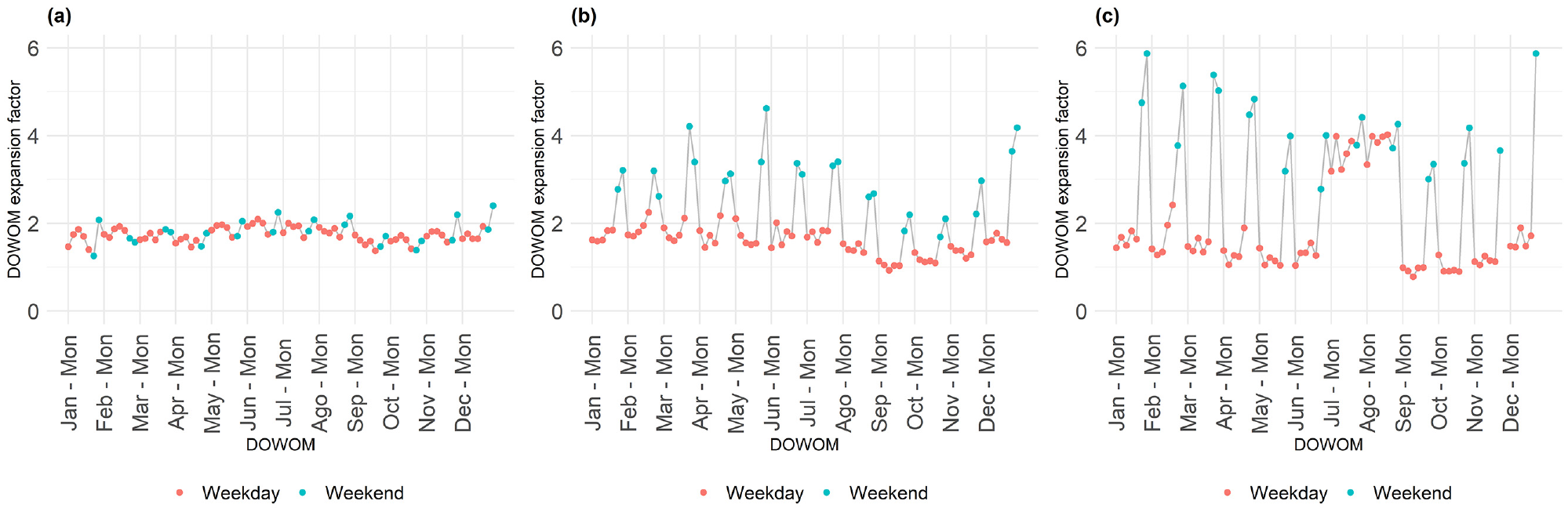
Different temporal pedestrian activity patterns for three different sites: (a) Fairway Road at Wilson Avenue, (b) King Street at Mt. Hope Street, and (c) Charles Street at Cameron Street.Note: DOWOM = day of week of month

Factor group #1 (Figure 2a) represents sites with consistent volumes on both weekdays and weekends throughout the year (i.e., low seasonality effects), implying probable associations with recreational and commercial activities because of the uniform exposure throughout the week. In contrast, Factor group #2 (Figure 2b) illustrates sites characterized by reduced volumes on weekends compared with weekdays (indicated by a high expansion factor value) and low seasonality effects, suggesting a correlation with working activities. Factor group #3 (Figure 2c) also exhibits reduced activity on weekends but demonstrates low pedestrian exposure during school holidays (July and August in Ontario, Canada), indicating a likely association with the presence of schools.

In addition to the three patterns identified in Figure 2, it was also observed that the pedestrian volume at some sites presents a seasonal trend. Figure 3 elaborates on this observation, illustrating two sites that exhibit characteristics of factor group #1 (i.e., consistent volumes on both weekdays and weekends). One site maintains a consistent volume throughout the year (Figure 3a), while the other experiences reduced volume during the winter season (Figure 3b). This seasonality is believed to be associated with the “level of obligation” associated with different types of trip-making. For example, mandatory trips, such as work-related activities or home grocery shopping, may contribute to consistent volumes, whereas discretionary trips may exhibit seasonality.

Figure 3.

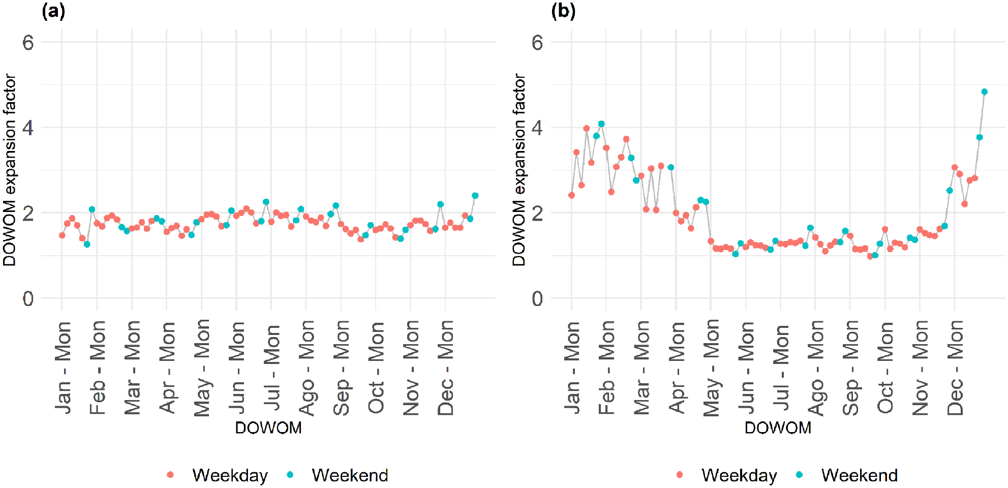
DOWOM expansion factors for two sites to show the effect of seasonality on pedestrian activity patterns: (a) Fairway Road at Wilson Avenue and (b) King Street at Highway 85 Ramp.Note: DOWOM = day of week of month

The same seasonality pattern was also noted in factor group #2 sites but not in factor group #3. This is expected from a phenomenological point of view: sites with pedestrian activity predominantly influenced by the presence of a nearby school are anticipated to have consistent volumes throughout the year, except for school holidays. The next subsection introduces the temporal indicators that are proposed to capture the identified patterns in both Figures 2 and 3.

Proposed Temporal Indicators for Identifying Factor Groups

Temporal indicators calculated using the DOWOM expansion factors of each site are proposed for the identification of factor groups. The median was consistently chosen over the mean in the development of these indicators. This choice aims to prevent the generation of potentially skewed indicators that might arise if the mean was employed.

The first indicator captures the level of similarity between weekdays and weekends. An adapted version of the weekend–weekday index (WWI), as proposed by Miranda-Moreno et al. ( 14 ), is proposed. The adapted WWI ( ${WWI}_{i}^{*}$ ) is computed in two steps. First, the ratio of expansion factors between weekends and weekdays for each month is computed using Equation 6. Second, the median of these monthly ratios is calculated (Equation 7). It is important to note that months affected by school holidays (i.e., July and August) were excluded from the analysis. This decision is based on the understanding that the weekend–weekday ratio during this period may not be representative at some sites.

The second indicator assesses the level of similarity between school holidays and typical periods through the school holiday–typical index (SHTI). SHTI is calculated as the ratio between the median of the expansion factors on weekdays during school summer holidays (the months of July and August) and the median of the expansion factors on weekdays during typical periods (Equation 8). In the context of this study, the typical period is defined as months not affected by the winter season, spanning from April to November.

The third and final indicator, named the deviation across months (DAM), is designed to capture seasonality through the magnitude of the deviation of expansion factors across months. DAM is computed in two steps. First, the expansion factor for each month is computed as the median of weekday factors for weekdays in that month (Equation 9). Second, the standard deviation of these monthly medians is calculated, considering all months except those affected by school holidays (Equation 10).

WWI*:

{WWI}_{i, m}^{*} = \frac{\frac{1}{2} \sum_{d = 6, 7} E F_{i, m, d}}{\frac{1}{5} \sum_{d = 1 - 5} E F_{i, m, d}}

(6)

{WWI}_{i}^{*} = media n_{m = 1 - 6, 9 - 12} (WW I_{i, m})

(7)

SHTI:

SHT I_{i} = \frac{media n_{m = 7 - 8; d = 1 - 5} (E F_{i, m, d})}{media n_{m = 4 - 6, 9 - 11; d = 1 - 5} (E F_{i, m, d})}

(8)

DAM:

E {F_{Typical}}_{i, m} = media n_{d = 1 - 5} (E F_{i, m, d})

(9)

DA M_{i} = standard deviatio n_{m = 1 - 6, 9 - 12} (E {F_{Typical}}_{i, m})

(10)

Where

$i$ = a given site

$m$ = month of year

$d$ = day of week (1 = Monday; 7 = Sunday)

$E F_{i, m, d}$ = DOWOM expansion factor at site $i$

$WW I^{*} =$ adapted weekend–weekday index

$SHTI$ = school holiday–typical index

$E F_{Typica l_{i, m}}$ = typical expansion factor at site and month

$DAM$ = deviation across months.

For all three indicators, the application of the above equations results in a value ≥ 0. To avoid biasing caused by very large values of the indicator, all indicators were truncated to a maximum value of 2.

These indicators considered school holidays and typical periods for the context of the Region of Waterloo. However, the conceptual framework is designed to be transferable to other jurisdictions. Practitioners can apply the temporal indicators by adjusting the months to align with the seasonal characteristics of a different jurisdiction.

Clustering Sites

The k-means clustering algorithm was utilized to group sites based on their similarity in the three temporal indicators defined in the previous section. The exploration of the optimal number of clusters (or factor groups) through the TWSS, silhouette test, and gap statistic indicated an optimal configuration with four or five factor groups. The choice of five groups was made as it aligned precisely with the factor groups previously visually identified. Table 1 summarizes the characteristics and number of sites for each factor group. The configuration with four groups erroneously combined sites from factor groups #4 and #5 into a single group.

Table 1.

Characteristics of Each Factor Group Based on Their Pedestrian Volume

Factor group	# sites	Similar on weekdays and weekends	Reduced on weekends	Constant throughout the year	Reduced in school holidays	Affected by seasonality¹
#1: Multipurpose	29	✓	X	✓	X	X
#2: Commuter	24	X	✓	✓	X	X
#3: Primarily school trips	15	X	✓	X	✓	X
#4: Discretionary multipurpose	7	✓	X	X	X	✓
#5: Discretionary commuter	3	X	✓	X	X	✓

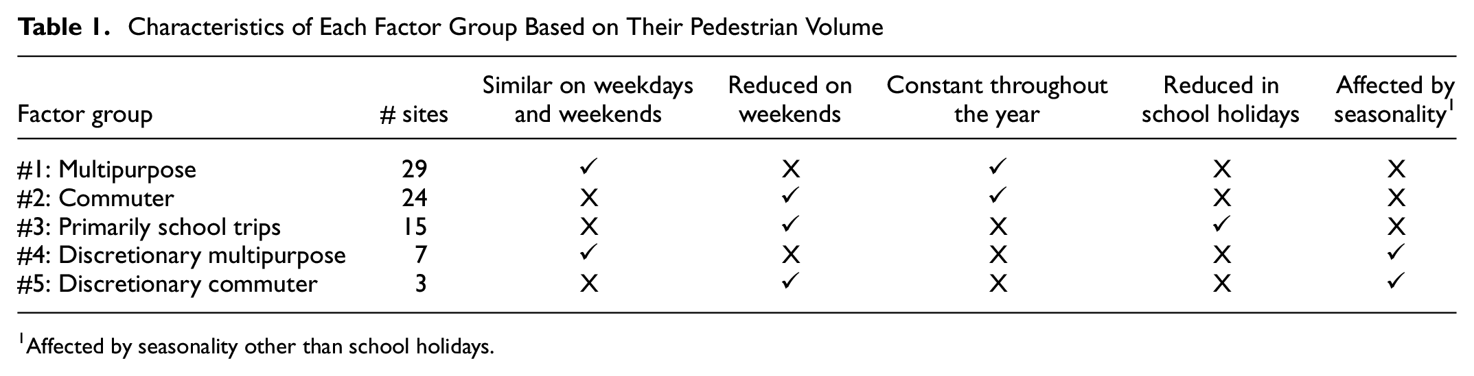
¹Affected by seasonality other than school holidays.

Figure 4 summarizes the DOWOM expansion factors for each of the factor groups identified in Table 1. The lines and dots in the figure represent the median of the factors within each group, while the grey background illustrates the 10th and 90th percentiles. The y-axis was limited to a value of 8, which is why the background is not displayed in some cases of Figure 4e. Consistent patterns are observed within each factor group, aligning with the traffic patterns that were visually identified. This consistency serves as an indication that the proposed temporal indicators effectively captured the characteristics of each site. The next subsection provides a characterization of the temporal indicators associated with each factor group.

Figure 4.

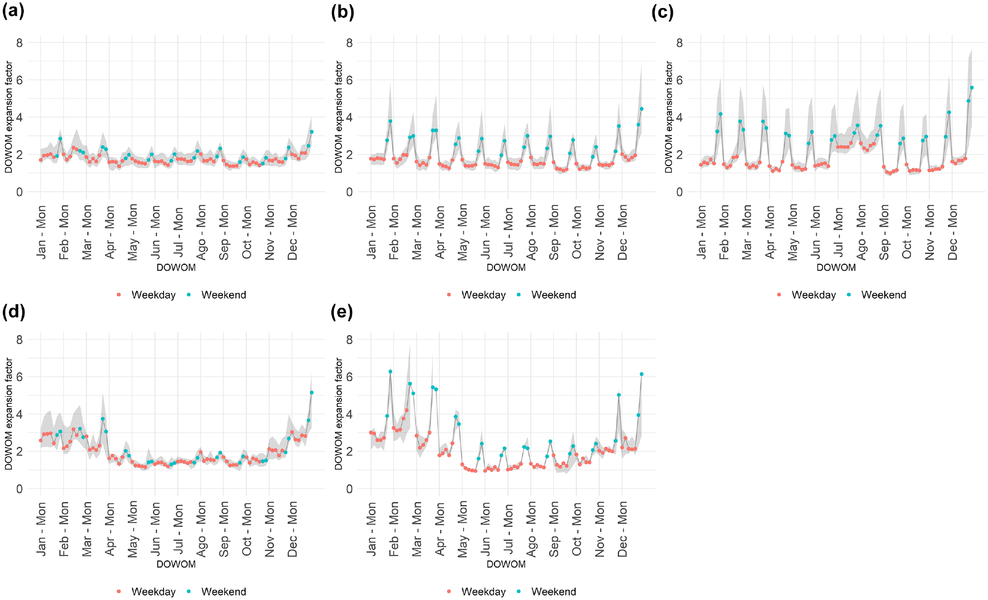
DOWOM expansion factor plots for factor groups identified through k-means clustering: (a) factor group #1 (29 sites), (b) factor group #2 (24 sites), (c) factor group #3 (15 sites), (d) factor group #4 (7 sites), and (e) factor group #5 (3 sites).

For comparison, Medury et al. ( 9 ) visually identified four factor groups based on hour-to-week expansion factors and using data from nine US states. The authors categorized these groups as urban commuter trails, central business districts, isolated recreational trails, or campgrounds/summer destinations. In contrast to our work, Medury et al. ( 9 ) observed sites where the volume on weekends was significantly greater than on weekdays, possibly because of the location of CC stations on recreational trails. In the Region of Waterloo, the CC stations are all located at signalized intersections and were primarily installed for signal timing and coordination purposes; they are positioned in urban—and likely commercial—areas. These locations are less likely to experience pedestrian travel patterns that are predominately recreational. Three sites present a WWI* lower than 1, with a minimum value of 0.83, indicating that weekend volumes were greater than weekday volumes on average. However, the values for the indicator were not low enough for the k-means algorithm to create a new factor group to represent “recreational” or “discretionary recreational” traffic patterns, and the sites were classified as multipurpose. It is possible, though, that these additional groups exist in the Region of Waterloo, but none of the sites monitored encompassed such characteristics.

In a separate study, Humagain and Singleton ( 10 ) identified five factor groups based on hour-to-week factors and three groups based on monthly patterns. The primary distinction among the hour-of-week groups lies in the number of observed intraday peaks: either one or two. Their analysis, conducted in Utah, U.S.A., did not reveal any sites with a greater volume on weekends compared with weekdays. Concerning the monthly patterns, one group showed the least variation throughout the year, another exhibited greater variation linked to weather sensitiveness, and a third displayed reduced activity during the summer months (June through August).

Temporal Indicator Thresholds for Identifying Factor Groups

This section introduces an additional step to the core method for identifying factor groups presented in the previous three sections. It assesses the possibility of identifying factor groups by applying thresholds to the temporal indicators. This alternative approach, which replaces the clustering technique with a simpler method, may prove useful for practitioners looking to replicate the results of this work. We acknowledge that further research is needed to assess the spatial transferability of these indicators and thresholds.

Using the factor group classification obtained from the k-means procedure as the “true” factor group, different combinations of thresholds were tested in search of the optimal configuration. Thresholds were tested in increments of 0.05, ranging from 1.2 to 1.8 for WWI* and SHTI and from 0.1 to 0.8 for DAM. All combinations were assessed based on the accurate labeling of sites.

The best combination of thresholds presented an almost perfect fit to the k-means classification. Out of 78 sites, only one site classified by the k-means clustering as factor group #1 was misclassified by the indicator thresholds method as #3. This indicates a strong separation of the factor groups based on their temporal indicators. Figure 5 illustrates a decision tree with the thresholds and the logic for classifying a given site into a factor group.

Figure 5.

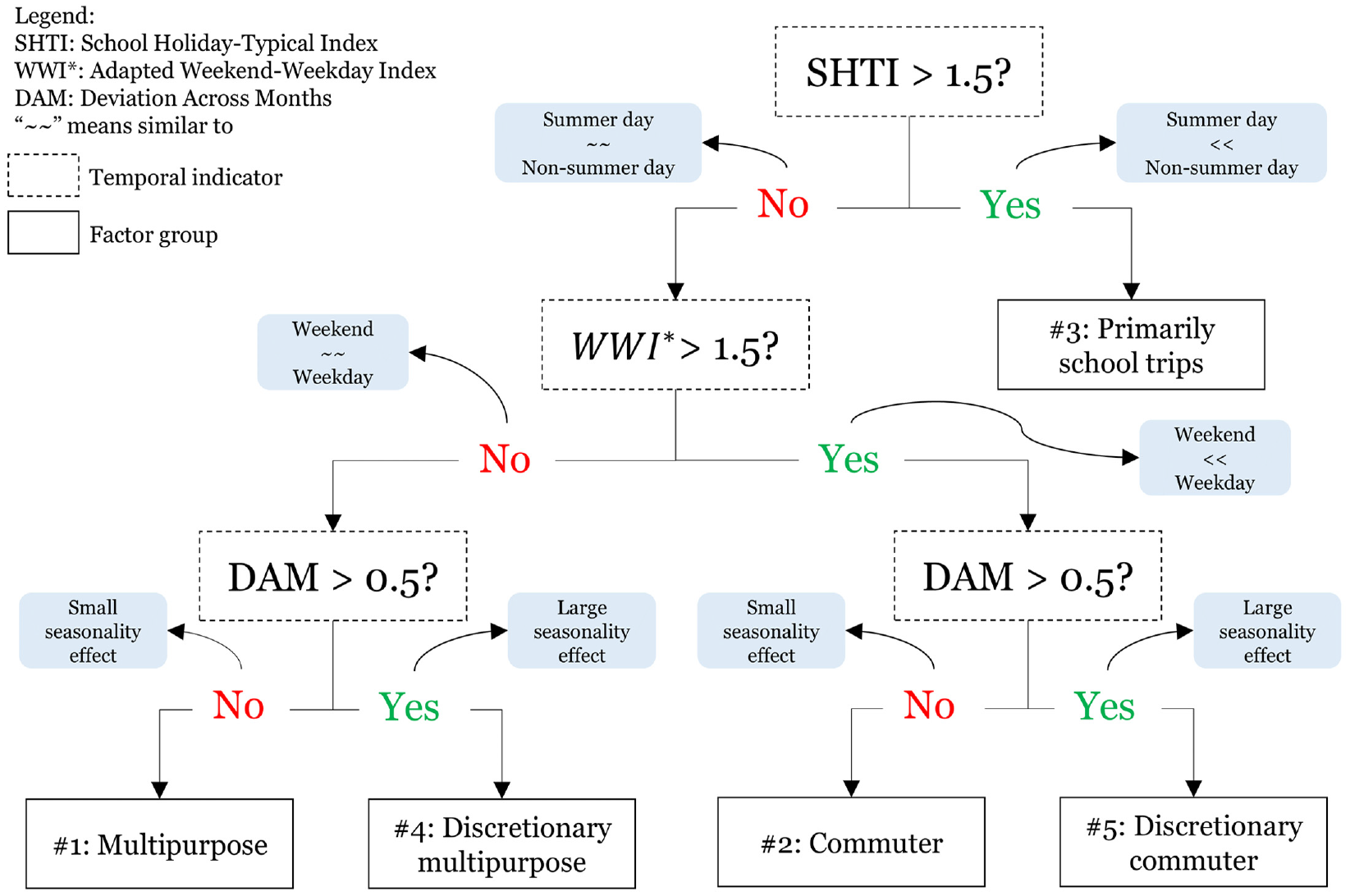
Decision tree: temporal indicator thresholds for identifying factor groups.

The first step in the classification process involves assessing whether the pedestrian volume at the site is primarily influenced by the presence of a school. If SHTI is greater than 1.5, then the site is associated with factor group #3. As discussed in the “Visual Inspection” section, sites where pedestrian activity is strongly linked to schools also exhibit reduced volumes on weekends and a steady pattern throughout the year. Therefore, there is no need to assess WWI* and DAM for these sites. If SHTI is less than 1.5, the subsequent steps involve assessing the values for WWI* and DAM to determine the site’s factor group. The factor group classification derived from the thresholds was applied in the following steps of this work.

To provide context for the thresholds used in other studies, Nordback et al. ( 11 ), while investigating non-motorized traffic (i.e., cyclists and pedestrians), employed WWI to categorize sites across six U.S. cities into three groups: weekday commute (average WWI ≤ 0.8), weekly multipurpose (0.8 < average WWI ≤ 1.2), and weekend multipurpose (average WWI > 1.2). According to the authors, no substantial month-to-month variation was observed, leading to the omission of monthly adjustments. Note that WWI is calculated based on actual volumes, whereas WWI* is derived from expansion factors. As a result, they possess inverse interpretations: a higher WWI indicates higher weekend traffic compared with weekdays, while a higher WWI* suggests higher weekday traffic relative to the weekend. Additional sources for thresholds can be found in the literature ( 6 , 7 , 14 ).

Modeling Factor Groups

After identifying the factor groups among the sites with CCs, the challenge lies in associating sites where only one or a few STCs are available with a specific factor group with the objective of employing an appropriate factor for expanding the STC to AADPT. To address this challenge, a multinomial logistic regression (MLR) is proposed to establish a link between each factor group (i.e., the dependent variable) and land-use, socioeconomic, and operational explanatory variables. The explanatory variables were collected within radii of 100, 200, 400, and 800 meters. The list of explanatory variables is provided in Table 2, as are descriptive statistics for each variable for a radius of 400 m.

Table 2.

Site Characteristic Variables and Descriptive Statistics for a Radius of 400 m

Variable	Unit	Source	Statistics (400 m radius)
Variable	Unit	Source	Avg.	SD	Min.	Max.
Pedestrian volume
AADPT	Volume per intersection	Jurisdiction	710	852	41	4,546
Land use
Commercial area (%)¹	%	Region of Waterloo Open Data Portal	38.9	24.2	0.0	85.6
Industrial area (%)¹	%		9.9	17.6	0.0	88.0
Residential area (%)¹	%		40.9	27.8	0.0	96.6
Park area	Square meters/1,000		22.8	35.0	0.0	174.6
School—all types	Count		0.8	1.2	0	5
School—high and post-secondary	Count		0.6	1.1	0	5
Places of worship	Count		2.1	2.8	0	12
Census-based
Employment density²	Employment per square km/1,000	Environics: 2020	3.5	2.9	0.0	13.1
Household income³	Median income per square km/1,000	Census: 2016	66.9	33.8	0.0	181.4
Household size³	Avg. number of people per household	Census: 2016	2.0	0.5	1.0	3.3
Population density³	Population per square km/1,000	Census: 2016	2.2	1.3	0.0	5.9
Walk to work (%)³	%	Census: 2016	11.0	9.2	0.0	32.6
Operational
Trails	Length (km)	Region of Waterloo Open Data Portal	0.7	0.7	0.0	2.7
Transit stops	Count		12.6	6.9	2	32

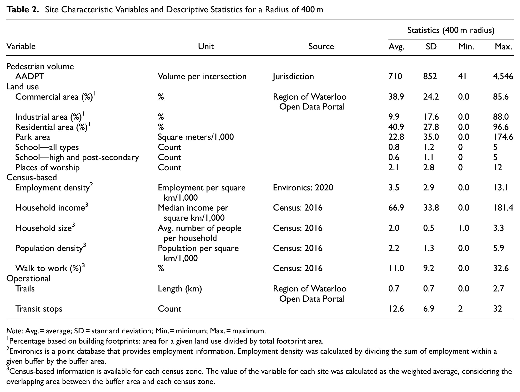
Note: Avg. = average; SD = standard deviation; Min. = minimum; Max. = maximum.

¹Percentage based on building footprints: area for a given land use divided by total footprint area.

²Environics is a point database that provides employment information. Employment density was calculated by dividing the sum of employment within a given buffer by the buffer area.

³Census-based information is available for each census zone. The value of the variable for each site was calculated as the weighted average, considering the overlapping area between the buffer area and each census zone.

A rule of thumb in the development of MLRs is to ensure that at least 10 observations are available for each class of dependent variables. However, factor groups #4 (discretionary multipurpose) and #5 (discretionary commuter) have seven and three observations, respectively. In light of this, it was decided to exclude group #5 from the analysis while retaining group #4. The model results were interpreted with caution, given the small sample size used for this group.

Fourteen explanatory variables (Table 2) were collected within four different radii. This resulted in the possibility of generating millions of variable sets, but testing each one is impractical. To address this, a simulation process was implemented with three steps. First, a radius was randomly assigned to each variable. Second, the linear correlation of every pair of variables was examined, and one variable of the pair was randomly removed if the correlation exceeded 0.50. Third, using the remaining variables, the MLR was calibrated using a stepwise process. The simulation was repeated 100,000 times. To identify the best model (or something close to it), the evaluation included the accuracy of classification (confusion matrix), McFadden pseudo-R², Akaike information criterion (AIC), and variance inflation factor (VIF). Additionally, a fivefold cross-validation procedure was employed to inspect the best model for overfitting and coefficient stability.

In anticipation of the detailed results discussed in the following section, it was observed that the magnitude of the error in expanding STCs of sites from factor group #3 (the group that is likely related to the presence of schools) is significantly higher than for sites from other factor groups. Consequently, it was decided to propose simpler approaches based on only two factor groups: one encompassing sites from factor groups #1, #2, and #4 and the other including sites from factor group #3. Three approaches were tested:

1) Binary logistic regression, following a procedure similar to MLR.

2) Presence of schools: A site is categorized as factor group #3 if there is a school within a specified radius. We considered two models: one considered the presence of any school; the other only high/post-secondary schools. Radii of 100, 200, 400, and 800 m were tested for optimal classification.

3) Presence of schools and commercial land use: A site is categorized as factor group #3 if there is a school (or high/post-secondary) within a specified radius and the percentage of commercial land use within a specified radius does not exceed a given percentage. The land-use constraint aims to minimize the misclassification of sites where the pedestrian activity is influenced not only by the nearby school but also by other land uses. Radii of 100, 200, 400, and 800 m and percentages from 0% to 100% in steps of 5% were tested to obtain optimal classification.

Multinomial Logistic Regression

Table 3 presents the MLR coefficients and odds ratios (ORs) of the best model obtained from the simulation approach described in the previous section. The OR is derived from the natural logarithm of the coefficient and should be interpreted as a comparison with the reference factor group. For instance, the OR of 4.181 for “Schools” in factor group #3 indicates that, while holding the other variables constant, a one-unit increase in the “Schools” variable makes the odds of the factor group being #3, on average, 4.181 times higher compared with factor group #1.

Table 3.

MLR Coefficients and Odds Ratio

Variable	Radius (m)	Factor group (reference: #1: Multipurpose)						VIF
		#2: Commuter		#3: Primarily school trips		#4: Discretionary multipurpose
		Coeff.	OR	Coeff.	OR	Coeff.	OR
Intercept	na	−0.597	na	1.048	na	2.389	na	na
Commercial area	400	−0.009	0.991	−0.091	0.913	−0.059	0.943	1.05
Industrial area	400	0.036	1.037	−0.065	0.937	0.087	1.091	1.05
Schools	400	1.034	2.812	1.431	4.181	−1.384	0.251	1.04
Transit stops	100	−0.068	0.934	0.091	1.095	−1.311	0.269	1.04
Accuracy of classification	69.3%
McFadden pseudo-R²	0.288
Sample size	75

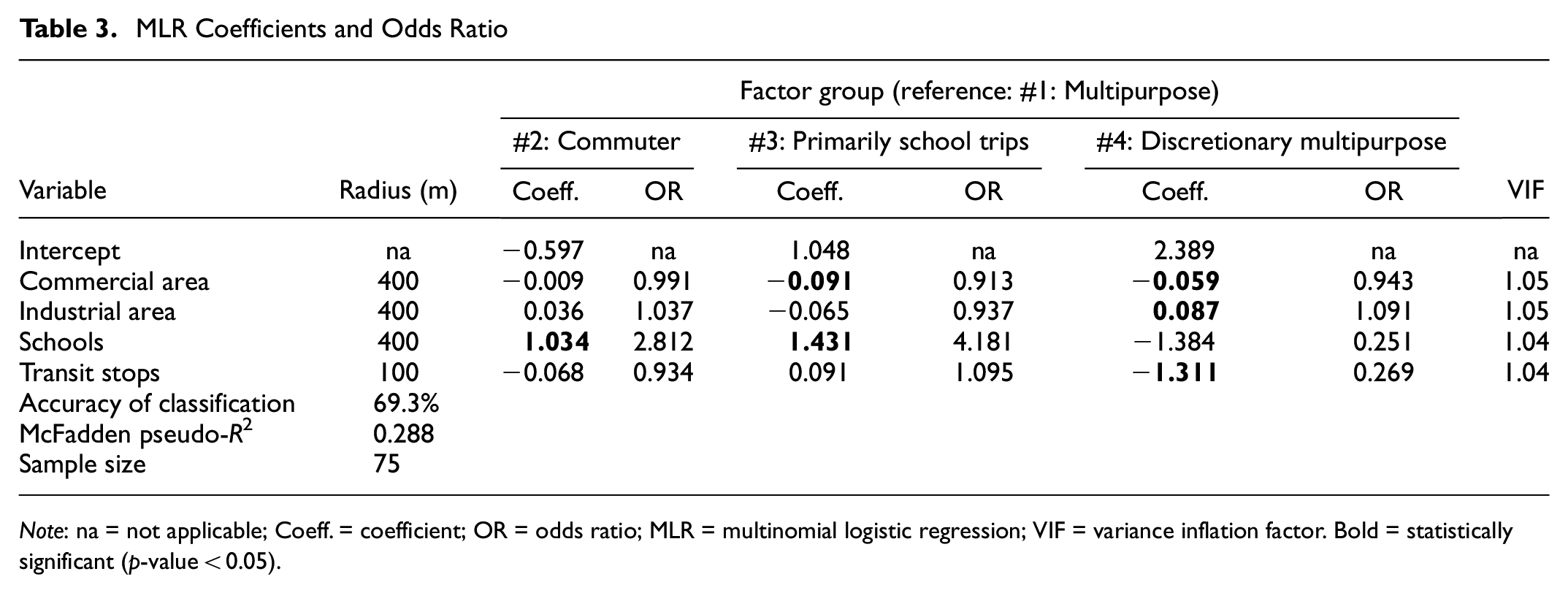
Note: na = not applicable; Coeff. = coefficient; OR = odds ratio; MLR = multinomial logistic regression; VIF = variance inflation factor. Bold = statistically significant (p-value < 0.05).

The overall accuracy of classification for the MLR using the entire dataset was 69.3%. In a fivefold cross-validation procedure run 100 times, the average training accuracy was 67.6%, while the average cross-validation accuracy was 57.2%. This suggests that the model is not overfitting. In a similar study, Medury et al. ( 9 ) achieved an overall accuracy of 67% when classifying four factor groups using MLR. Furthermore, our model presented low VIF values for all variables, suggesting the absence of multicollinearity.

The selected model is simple, involving only four explanatory variables. We were able to generate more complex models with an accuracy of classification around 85%; however, these models exhibited overfitting and stability of coefficient issues, likely caused by the relatively small sample size used for calibration.

The interpretation of the model coefficients shows interesting findings. The variable “Commercial area” exhibits a negative coefficient for factor groups #2 and #3, indicating that factor group #1 is linked to commercial activity. This matches expectations, given the characteristic of a consistent pedestrian volume throughout the week in factor group #1 and reduced volumes on weekends in factor groups #2 and #3. However, the presence of a statistically significant and negative coefficient for factor group #4 lacks clarity from a phenomenological perspective. Factor groups #1 and #4 share the feature of having a relatively consistent volume throughout the week, but they are different in the seasonality aspect. As a result, it would be expected that factor group #4 is also associated with a certain level of commercial activity. A potential approach for addressing this could involve segregating commercial land use to distinguish establishments based on their “attendance patterns.” For instance, differentiating between grocery stores, which likely maintain a more constant activity throughout the year (i.e., factor group #1), and pubs or restaurants, which might experience more seasonal variations (i.e., factor group #4). Increasing the precision in categorizing land use could potentially lead to a more comprehensible interpretation of the outcomes, but it requires more disaggregated and sophisticated land-use databases. Humagain and Singleton ( 10 ) also reported a significant negative coefficient for “Commercial area” associated with their monthly factor group that was affected by seasonality, though they did not provide a detailed interpretation.

The positive coefficient associated with the variable “Industrial area” for factor group #2 is expected, although it is not statistically significant at a 95% degree of confidence. This expectation arises from the decreased pedestrian activity on weekends. Meanwhile, the coefficient for factor group #4 may be interpreted as indicative of commuting seasonality: individuals may choose to take public transportation and/or walk to work in months unaffected by severe cold but to opt for driving or carpooling during winter months. This observation aligns with the findings of Humagain and Singleton ( 10 ), who found a similar outcome in their monthly factor group affected by seasonality, showing a correlation with increased employment density.

The presence of schools indicates associations with factor groups #2 and #3, albeit with a stronger relation to factor group #3, as anticipated. The positive and significant coefficient for factor group #2 can be understood as intersections with nearby schools in which the pedestrian activity is not mainly dictated by the school to the extent of observing substantial changes during school holidays. This may be linked to either or both the type and size of school (e.g., large high schools are expected to generate more pedestrian activity than smaller primary schools) and the presence of other land uses that generate pedestrian trips.

The negative and significant coefficient of the variable “Transit stops” for factor group #4 indicates that sites with nearby transit stops are associated with more consistent traffic patterns throughout the year. This aligns with expectations, considering that transit stops are part of the means of transportation. Thus, it is expected that the “attendance pattern” generated by a transit stop would be steadier than that of a commercial land use, for example.

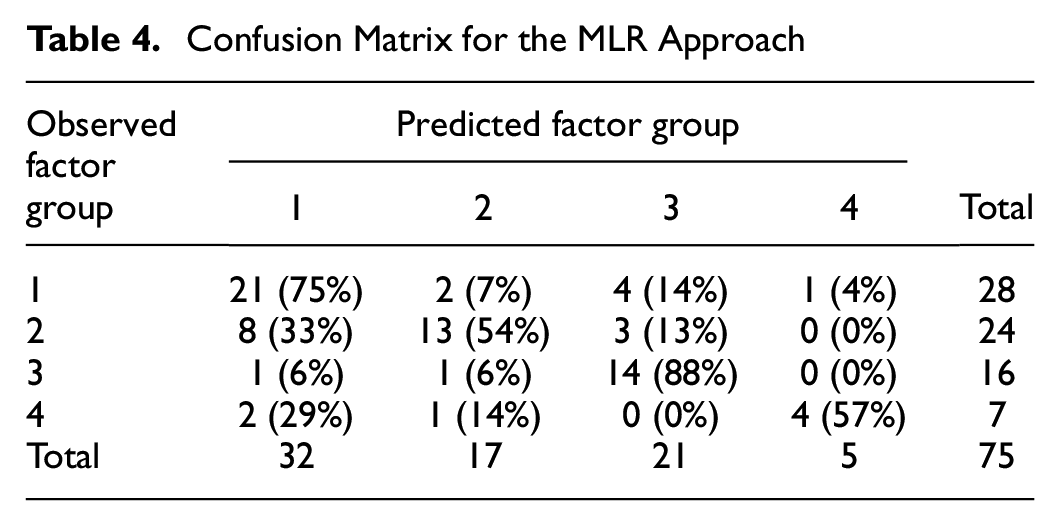
Table 4 presents the confusion matrix for the MLR. “Observed factor group” in this table is the factor group assigned by the temporal indicator threshold method. The information in parentheses represents the value of the cell divided by the total number of sites observed in each factor group. Overall, the classification errors are evenly distributed across the matrix, except for one cell: among the 24 sites classified by the temporal indicator threshold method in factor group #2, 8 were incorrectly predicted to belong to factor group #1. Further examination of these sites reveals that half of them have WWI* values falling between 1.50 and 1.60. The WWI* threshold distinguishing groups #1 and #2 is set at 1.50 (Figure 5). This indicates that these particular sites are in a transitional area, sharing characteristics of both groups. Consequently, it is not expected that using expansion factors from factor group #1 instead of factor group #2 would significantly degrade the accuracy of the estimated AADPT for these sites.

Table 4.

Confusion Matrix for the MLR Approach

Observed factor group	Predicted factor group				Total
Observed factor group	1	2	3	4	Total
1	21 (75%)	2 (7%)	4 (14%)	1 (4%)	28
2	8 (33%)	13 (54%)	3 (13%)	0 (0%)	24
3	1 (6%)	1 (6%)	14 (88%)	0 (0%)	16
4	2 (29%)	1 (14%)	0 (0%)	4 (57%)	7
Total	32	17	21	5	75

Logistic Regression and School-Based Approaches

The calibration of logistic regression (LR) was conducted based on two categories: (I) a combination of factor groups #1, #2, and #4 (called non-school trips), and (II) factor group #3 (primarily school trips). In Table 5, LR coefficients and ORs are presented. The overall accuracy of classification using the entire dataset reached 92.0%. In the fivefold cross-validation procedure executed 100 times, the average training accuracy was 91.4%, while the average cross-validation accuracy was 84.7%. These results suggest that the model is not overfitting. Additionally, the greatest VIF value of 3.86 is relatively far from the value of 5 normally considered for flagging multicollinearity.

Table 5.

Logistic Regression Coefficients and Odds Ratios for Factor Group #3 (Primarily School Trips)

Variable	Radius (m)	Coeff.	OR	VIF
Intercept	na	−9.820	na	na
Commercial area	200	−0.154	0.857	3.86
Employment density	100	0.173	1.189	2.26
Household size	800	4.430	83.923	3.07
Places of worship	200	0.801	2.227	2.33
Schools	800	0.806	2.239	2.99
Accuracy of classification	92.0%
McFadden pseudo-R²	0.486
Sample size	75

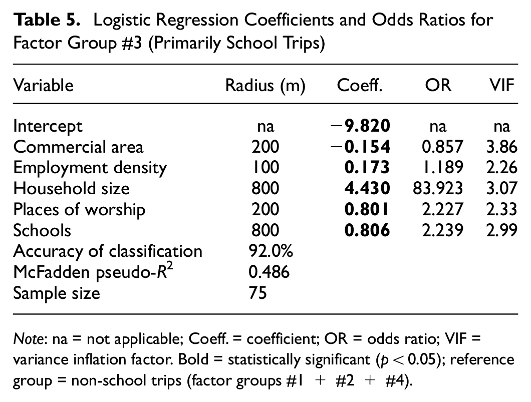
Note: na = not applicable; Coeff. = coefficient; OR = odds ratio; VIF = variance inflation factor. Bold = statistically significant (p < 0.05); reference group = non-school trips (factor groups #1 + #2 + #4).

Variables such as “Commercial area” and “Schools,” which were statistically significant for factor group #3 in the MLR (Table 3), are also observed to be significant in the LR. The simplicity of the model (i.e., two dependent variables instead of four) allowed the inclusion of additional explanatory variables without causing overfitting issues. The variables are “Employment density,”“Household size,” and “Places of worship.”

In the context of the school-based approaches, the simplest approach that relies solely on the presence of schools within a given radius demonstrated that the variable “Schools—all types” within a 400-m radius yielded the highest classification accuracy, at 72.0%. Concerning the school-based approach that also considers the percentage of commercial land use, the combination of the variables “Schools—all types” and “Commercial area” within the same 400-m radius and with a threshold set at 50% provided the highest accuracy of 84.0%. This means that for a site to be classified into factor group #3, it must have at least one school within a 400-m radius, and the percentage of commercial land use within the same radius must be below 50%.

Table 6 presents the confusion matrices for the LR and school-based approaches. Overall, all three approaches exhibit similar classification for the sites of factor group #3, with the school-based approaches slightly outperforming the LR (13 versus 12). Conversely, the LR demonstrates superior performance in correctly classifying sites in the combined factor group (57 versus 50 versus 41). Comparing the two school-based approaches, the 13 sites correctly identified as factor group #3 are identical in both approaches. Additionally, it is observed that the inclusion of the commercial land-use constraint was beneficial for accurately classifying sites in the combined factor group (50 versus 41). This suggests that there are indeed sites with nearby schools whose pedestrian activity is not primarily influenced by the schools.

Table 6.

Confusion Matrices for Logistic Regression (LR) and School-Based Approaches

Observed factor groups	Approach / predicted factor groups
	LR		Schools and commercial		Schools		Total
	#1+#2+#4	#3	#1+#2+#4	#3	#1+#2+#4	#3	Total
#1+#2+#4	57 (97%)	2 (3%)	50 (85%)	9 (15%)	41 (69%)	18 (31%)	59
#3	4 (25%)	12 (75%)	3 (19%)	13 (81%)	3 (19%)	13 (81%)	16
Total	61	14	53	22	44	31	75

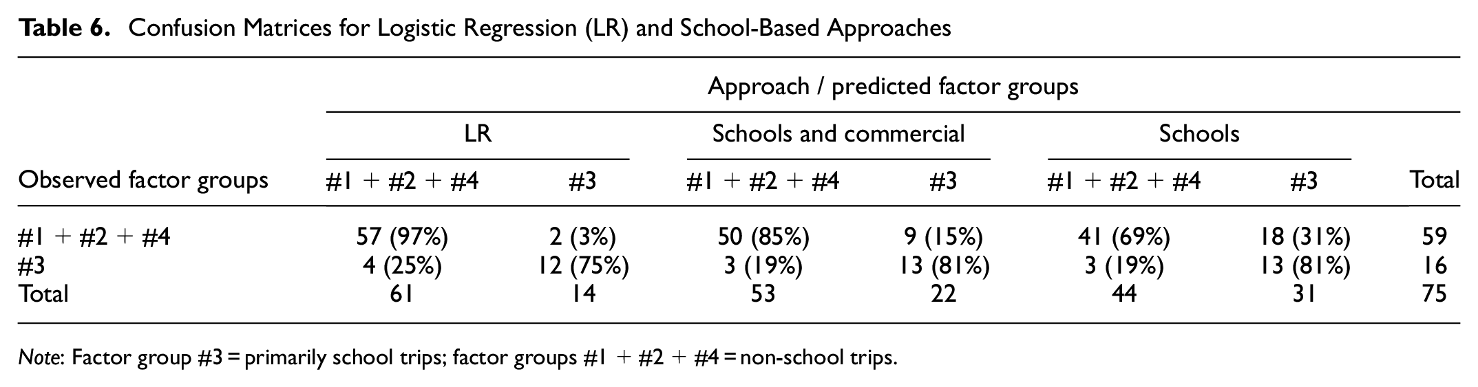
Note: Factor group #3 = primarily school trips; factor groups #1+#2+#4 = non-school trips.

Assessing the Accuracy of Expanding STCs to AADPT

Inspired by the methodology introduced by Medury et al. ( 9 ), five different methods for assigning sites to factor groups were considered in the assessment of the expansion of the STCs to AADPT:

1) From STC site method: In this method, both the STC and the expansion factor originate from the same site. This represents the best expansion possible considering the use of DOWOM factors. In this case, every site represents one factor group. This method cannot be used in practice because expansion factors cannot be computed for STC sites.

2) Naïve method: This method employs a single expansion factor for each DOWOM, determined as the average of the expansion factors across all sites. It represents the worst expansion possible, with all sites grouped into a single factor group.

3) Empirical factor group method: Sites are categorized into factor groups based on their temporal indicator threshold classification. Although this method cannot be used in practice (because clustering on the basis of temporal indicators can only be done for CC sites, not for STC sites), this method eliminates modeling error, allowing for the identification of sources of error such as combining sites into factor groups and assigning STC sites to factor groups via models.

4) Predicted factor group—maximum probability: MLR and LR outcomes provide probabilities of a site belonging to a specific factor group. This approach assumes that the DOWOM expansion factor is selected from the factor group with the highest probability.

5) Predicted factor group—weighted probability: Unlike the previous approach, this method does not directly assign an STC site to a particular factor group. Instead, it calculates the DOWOM expansion factor based on the weighted average of the DOWOM expansion factors from each factor group, where the weights are the probabilities derived from MLR and LR outcomes.

Table 7 summarizes the performance of the expansion of STCs to AADPT by considering the various approaches (i.e., MLR, LR, and school-based) and site assignment methods listed above. The MAPE for each approach was derived using a process similar to the one employed for the initial determination of the appropriate type of expansion factor (Equations 1–5). The results are categorized based on the strategy type (i.e., four or two factor groups) and on the potential days for the collection of STCs (i.e., all days or candidate days). Additionally, the MAPE values for certain approaches are shown as the difference from the naïve method. For instance, an overall value of −2.6 for the empirical factor group method using candidate days indicates that the MAPE for this method is 17.6% (calculated as 20.2% minus 2.6%). Figure 6 displays the DOWOM expansion factors for each factor group and strategy type, with days considered as candidates highlighted in pink. The expansion factors for the naïve method are also included. The highlights from Table 7 and Figure 6 are presented and discussed below:

Candidate days versus all days: Consistently improved performance is noted when restricting the analysis to candidate days. This is a well-established finding, as it aligns with the understanding that pedestrian activity on typical days exhibits less variability compared with when all days are considered. For example, pedestrian volume on Tuesdays in April tends to be more stable than that on Saturdays in December.

Expansion factor from STC site method: The observed MAPEs of 13.2% (candidate days) and 16.8% (all days) represent the best possible performance when using DOWOM factors. This error corresponds to the variability of the STC within each DOWOM.

Naïve method versus empirical factor group method:

○ Overall, employing the empirical factor group method yields somewhat modest improvements compared with the naïve method. For instance, when considering candidate days and employing four factor groups, the MAPE for the naïve method (worst performance) is 20.2% and the MAPE when the expansion factor is computed from the STC site (best performance) is 13.2%. Thus, at best there is an opportunity to improve on the MAPE of the naïve method by 7%. Employing the empirical factor group method to group the sites and utilizing the expansion factor from the correct site only reduces the naïve method MAPE by 2.6% (a 12.9% reduction in error). This indicates that the remaining 4.4% of the MAPE is attributed to the variation within sites of the same factor group.

○ Candidate days and four factor groups: Factor group #3 exhibits the highest sensitivity to correct classification, as evidenced by the substantial error associated with the naïve method and the notable improvement when applying the empirical factor group method. This sensitivity motivated the alternative proposal of having only two factor groups.

○ Clustering factor groups #1, #2, and #4 into a single factor group worsened the empirical factor group method results (it increased the magnitude of MAPE by 1.2% for candidate days and 2.0% for all days).

○ Candidate days and two factor groups: It was unexpected that the empirical factor group method produced a poorer result than the naïve method for the combined factor group. A detailed exploration revealed two causes contributing to this result: (I) the method of calculating the MAPE overestimates the influence of relatively large STCs, and (II) the expansion factors derived from the naïve method consistently exhibited lower values (averaging 8% lower) compared with the factors obtained from the combined factor group (Figure 6b). The effect of these two causes is illustrated using a simple example. Consider a hypothetical scenario where a site with an AADPT of 300 has two STCs, one with a volume of 100 and the other with a volume of 200. The specific (or DOY) expansion factor is 3.0 (300/100) for the former and 1.5 (300/200) for the latter. The average expansion factor for this situation is 2.25. Applying this factor for the two STCs generates absolute percent errors of 25% and 50%, with a resulting MAPE of 37.5%. If the averaged expansion factor is reduced by 8%, bringing it to 2.07, we expect the resulting MAPE to be larger than 37.5%. However, the resulting absolute percent errors became 31% and 38%, resulting in a lower MAPE of 34.5%. This example illustrates that the unexpected result is derived from a limitation in how the MAPE is calculated. To further support this finding, when considering all days, the empirical factor group method outperforms the naïve method.

MLR method:

○ Using the MLR method to identify the factor group provides a 1.2% reduction in the MAPE compared with the naïve method (candidate days). This improvement is relatively modest when contrasted with the naïve method. This aligns with the findings of Medury et al. ( 9 ), who reported comparable magnitudes of improvement. However, the significance of these improvements becomes more apparent when contextualized within the “room for improvement” between the best and worst methods, which is calculated as 7% (20.2% minus 13.2%) for candidate days. In this context, a 1.2% improvement translates to 17% of the total potential improvement that could have been attained.

○ Candidate days: A comparison with the empirical factor group method, which essentially represents the outcomes of a perfect model, reveals that 1.4% of the MAPE (2.6% minus 1.2%) can be attributed to model misclassification (i.e., the MLR predicts the incorrect factor group).

○ The poor performance of factor group #2, particularly for the maximum probability method, can be linked to the relatively poor classification of sites within this group (Table 4).

LR method and school-based approaches:

○ The school-based approaches exhibit superior performance compared with the LR method for factor group #3. This is attributed to the slightly more accurate predictions for sites within factor group #3 achieved with the school-based approaches than with the LR method (Table 6).

○ In the context of using candidate days, for which expansion factor values are relatively similar across factors groups (Figure 6b), the misclassification of sites in the combined factor group (Table 6) does not substantially degrade the performance of the school-based approaches, resulting in comparable performance to that of the LR method. Conversely, when considering all days, the significance of the misclassification becomes more apparent. This is caused by the more substantial difference in expansion factors between the combined factor group and factor group #3 in this scenario (Figure 6b).

Overall evaluation:

○ The weighted-probability MLR method typically exhibits slightly superior performance compared with the maximum-probability MLR method, a trend consistent with the findings of Medury et al. ( 9 ).

○ Results obtained from the MLR and LR methods demonstrate comparability in both candidate days and all days. This suggests that developing a model that focuses on identifying sites associated with schools may be sufficiently effective when contrasted with a more complex approach that considers all existing traffic patterns.

○ In the context of using candidate days, the performance of the school-based approaches is comparable to those of the MLR and LR methods. As discussed, this happens because the misclassification of sites from the combined factor group does not degrade model accuracy when only candidate days are considered. Conversely, the performance of the school-based approaches is degraded when using all days.

Figure 6.

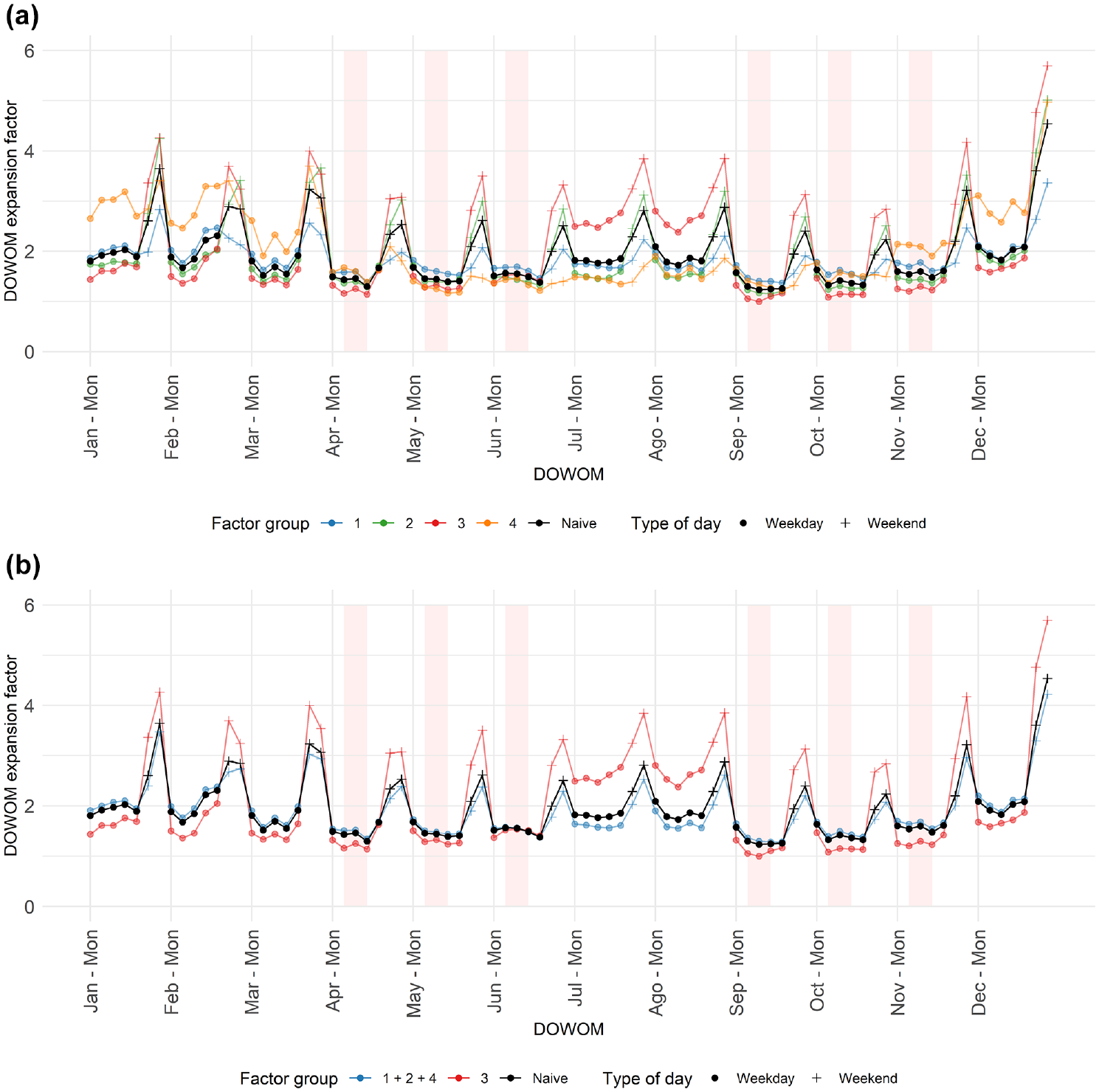
DOWOM expansion factors per factor group for (a) four factor groups and (b) two factor groups.

Table 7.

Expanding STC to AADPT: Summary of Results

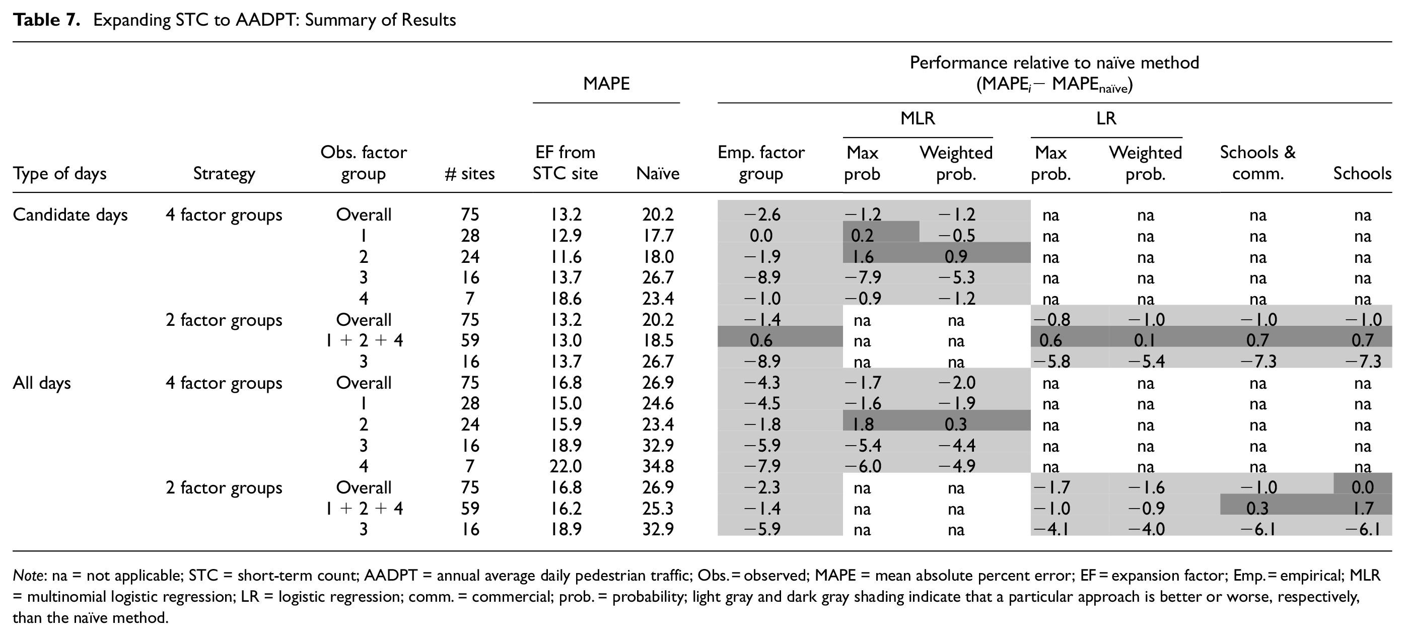
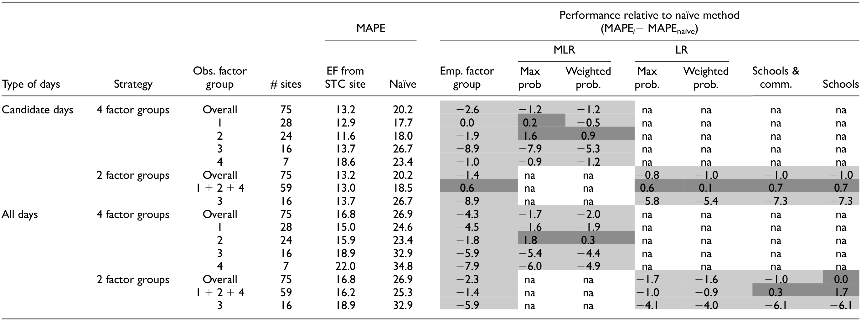
Note: na = not applicable; STC = short-term count; AADPT = annual average daily pedestrian traffic; Obs. = observed; MAPE = mean absolute percent error; EF = expansion factor; Emp. = empirical; MLR = multinomial logistic regression; LR = logistic regression; comm. = commercial; prob. = probability; light gray and dark gray shading indicate that a particular approach is better or worse, respectively, than the naïve method.

Conclusions and Practical Recommendations

This work examined the expansion of pedestrian STCs to AADPT at intersections. It followed a procedure that involved the identification of factor groups, the calibration of models to associate sites where long-term volumes are not available with factor groups, and the measurement of the error related to the expansion, considering approaches with different levels of complexity.

Five factor groups were visually identified, and then three temporal indicators were proposed to characterize them: WWI*, SHTI, and DAM. The use of thresholds for these indicators allowed for an adequate representation of the factor groups. Further research is required to assess the spatial transferability of these indicators and thresholds. Additionally, none of the sites considered in this work presented a primarily recreational pattern (i.e., pedestrian volume on weekends is greater than on weekdays). So, it is possible—and likely—that extra factor groups representing pedestrian volumes predominantly associated with recreational trips may exist in the Region of Waterloo and in other jurisdictions.

An MLR was developed to link factor groups to land-use, socioeconomic, and operational attributes. Explanatory variables that represent commercial area, industrial area, number of schools, and number of transit stops were found to be significant. The MLR provided a reasonable accuracy of classification of 69.3%. Although this performance is consistent with magnitudes reported in the literature, we believe that an improved model could have been developed if a larger sample size was available, especially for factor groups #4 and #5.

In addition to the MLR, three simpler approaches were also proposed, with the focus of identifying sites where pedestrian activity is highly influenced by the presence of schools (i.e., factor group #3). An LR and two school-based approaches were developed and demonstrated good accuracy of classification (I) overall (72%–92%) and (II) for factor group #3 (75%–81%).

The assessment of the expansion of STCs to AADPT considered other methods (for reference) in addition to the modeling approaches aforementioned, including (I) the naïve method (which averaged the expansion factor across all sites, representing the worst scenario), (II) the empirical factor group method (which averaged the expansion factor across sites that belong to a given factor group), and (III) the from STC site method (both the STC and expansion factor originate from the same site, representing the best scenario). Overall, modest improvements to the MAPE on the order of 0.8%–1.2% were obtained when using the modeling approaches in comparison with the naïve method when considering candidate days. The significance of these improvements is more noticeable when contextualized within the room for improvement between the best and worst methods, which is calculated as a MAPE of 7%. In this regard, the improvements are on the order of 11%–17%.

More importantly, different magnitudes of error were observed across factor groups, with factor group #3 (sites for which pedestrian volumes are primarily associated with trips to/from school) being the one with the highest error when considering candidate days. This means that the simple naïve method provided reasonable results for most of the factor groups, suggesting that—if data and/or personnel resources are constrained—practitioners may concentrate their efforts on identifying the sites affected by the presence of schools.

We make the following recommendations for practitioners who need to expand pedestrian STCs to AADPT:

1) As established in the literature, this work reinforces the use of STCs from days with typical pedestrian activity rather than STCs from any day throughout the year.

2) If a jurisdiction has sufficient CC stations (i.e., 10 or more stations per factor group) and qualified personnel to develop statistical models, the development of an MLR is recommended, as this approach has been demonstrated to provide the best results.

3) If a jurisdiction lacks sufficient CC stations for developing an MLR (i.e., less than 10 stations per factor group), it is suggested that of the proposed simpler approaches be applied. This is possible if CCs are deployed at sites that are affected by schools.

a. If STCs from all days are used, the LR method is recommended.

b. If STCs from candidate days are used, the school-based approaches are recommended as they provide comparable accuracy and are much simpler to apply.

4) If a jurisdiction lacks any CC stations but is willing to install the minimum number possible, it is recommended to strategically deploy CC stations in at least five sites ( 11 ) of two distinct groups based on the degree of pedestrian activity affected by schools (i.e., highly affected and not affected). This should be sufficient for employing the school-based approaches if STCs from candidate days are used.

Footnotes

Acknowledgements

The authors gratefully acknowledge (I) the Region of Waterloo for providing permission to use the pedestrian volume data and for providing rich, open data portals that were essential sources of information for this research and (II) Miovision for providing access to the pedestrian data.

Author Contributions

The authors confirm contribution to the paper as follows: study conception and design: L. T. P. Sobreira, B. Hellinga; data collection: L. T. P. Sobreira, B. Hellinga; analysis and interpretation of results: L. T. P. Sobreira, B. Hellinga; draft manuscript preparation: L. T. P. Sobreira, B. Hellinga. All authors reviewed the results and approved the final version of the manuscript.

Declaration of Conflicting Interests

The author(s) declared no potential conflicts of interest with respect to the research, authorship, and/or publication of this article.

Funding

The author(s) disclosed receipt of the following financial support for the research, authorship, and/or publication of this article: the authors gratefully acknowledge financial support from Transport Canada and Natural Sciences and Engineering Research Council of Canada (NSERC).

ORCID iDs

Lucas Tito Pereira Sobreira

Bruce Hellinga

The work in this paper reflects the views of the authors and there is no explicit or implicit endorsement by any of the aforementioned jurisdictions/companies. The research was carried out by the authors and no endorsement of the methods or findings by funding agencies is claimed or implied.

References

Stipancic

Miranda-Moreno

Strauss

Labbe

Pedestrian Safety at Signalized Intersections: Modelling Spatial Effects of Exposure, Geometry and Signalization on a Large Urban Network. Accident Analysis & Prevention, Vol. 134, 2020, p. 105265. https://doi.org/10.1016/j.aap.2019.105265.

Munira

Sener

I. N.

Dai

A Bayesian Spatial Poisson-Lognormal Model to Examine Pedestrian Crash Severity at Signalized Intersections. Accident Analysis & Prevention, Vol. 144, 2020, p. 105679. https://doi.org/10.1016/j.aap.2020.105679.

Molino

J. A.

Kennedy

J. F.

Johnson

P. L.

Beuse

P. A.

Emo

A. K.

Pedestrian and Bicyclist Exposure to Risk: Methodology for Estimation in an Urban Environment. Transportation Research Record: Journal of the Transportation Research Board, 2009. 2140: 145–156.

Grossman

Rodgers

M. O.

Guensler

Watkins

If Safety Matters, Let’s Measure It: Nationwide Survey Results for Bicycle and Pedestrian Treatment Prioritization. Journal of Transportation Engineering, Part A: Systems, Vol. 145, No. 1, 2019. https://doi.org/10.1061/JTEPBS.0000205.

FHWA. Traffic Monitoring Guide. Federal Highway Administration, Office of Highway Information Management, 2016.

Hankey

Lindsey

Marshall

Day-of-Year Scaling Factors and Design Considerations for Nonmotorized Traffic Monitoring Programs. Transportation Research Record: Journal of the Transportation Research Board, 2014. 2468: 64–73.

Johnstone

Nordback

Kothuri

Annual Average Nonmotorized Traffic Estimates from Manual Counts: Quantifying Error. Transportation Research Record: Journal of the Transportation Research Board, 2018. 2672: 134-144.

Nordback

Johnstone

Kothuri

Optimizing Short Duration Bicycle and Pedestrian Counting in Washington State. Research Report WA-RD 875.2. Washington State Department of Transportation, 2017.

Medury

Griswold

J. B.

Huang

Grembek

Pedestrian Count Expansion Methods: Bridging the Gap Between Land Use Groups and Empirical Clusters. Transportation Research Record: Journal of the Transportation Research Board, 2019. 2673: 720–730.

10.

Humagain

Singleton

P. A.

Advances in Pedestrian Travel Monitoring: Temporal Patterns and Spatial Characteristics Using Pedestrian Push-Button Data from Utah Traffic Signals. Journal of Transport and Land Use, Vol. 14, No. 1, 2021, pp. 1341–1360. https://doi.org/10.5198/jtlu.2021.2112.

11.

Nordback

Kothuri

Johnstone

Lindsey

Ryan

Raw

Minimizing Annual Average Daily Nonmotorized Traffic Estimation Errors: How Many Counters Are Needed per Factor Group?

Transportation Research Record: Journal of the Transportation Research Board, 2019. 2673: 295–310.

12.

Turner

Lasley

Strategic Plan for Non-Motorized Traffic Monitoring in Colorado. Texas Transportation Institute, College Station, 2012.

13.

Hernández-Vega

Matamoros-Jiménez

Clustering Approach to Generate Pedestrian Traffic Pattern Groups. Ciencia e Ingeniería Neogranadina, Vol. 31, No. 2, 2021, pp. 41–59. https://doi.org/10.18359/rcin.4403.

14.

Miranda-Moreno

Nosal

Schneider

Proulx

Classification of Bicycle Traffic Patterns in Five North American Cities. Transportation Research Record: Journal of the Transportation Research Board, 2013. 2339: 68–79.

15.

Lindsey

Petesch

Hankey

The Minnesota Bicycle and Pedestrian Counting Initiative: Implementation Study. Research Report Number MN/RC 2015-34. Minnesota Department of Transportation, 2015.

16.

Singleton

P. A.

Runa

Pedestrian Traffic Signal Data Accurately Estimates Pedestrian Crossing Volumes. Transportation Research Record: Journal of the Transportation Research Board, 2021. 2675: 429–440.

17.

Weather Spark. Climate and Average Weather Year Round in Waterloo. 2023. https://weatherspark.com/y/19227/Average-Weather-in-Waterloo-Canada-Year-Round. Accessed December 5, 2023.

18.

Nosal

Miranda-Moreno

L. F.

Krstulic

Incorporating Weather: Comparative Analysis of Annual Average Daily Bicyclist Traffic Estimation Methods. Transportation Research Record: Journal of the Transportation Research Board, 2014. 2468: 100–110.

Expanding Short-Term Pedestrian Volume Counts to Average Annual Daily Counts at Intersections: Temporal Pattern Indices and a Comparison of Statistical Land Use and Simple Threshold Methods

Abstract

Keywords

Objectives

Work Structure

Data Sources

Assessing Types of Expansion Factors

Identifying Factor Groups

Visual Inspection

Proposed Temporal Indicators for Identifying Factor Groups

Clustering Sites

Temporal Indicator Thresholds for Identifying Factor Groups

Modeling Factor Groups

Multinomial Logistic Regression

Logistic Regression and School-Based Approaches

Assessing the Accuracy of Expanding STCs to AADPT

Conclusions and Practical Recommendations

Footnotes

Acknowledgements

Author Contributions

Declaration of Conflicting Interests

Funding

ORCID iDs

References