Computationally Efficient Approach for Evaluating Eco-Approach and Departure for Heavy-Duty Trucks

Abstract

Connected vehicle-based eco-driving applications have emerged as effective tools for improving energy efficiency and environmental sustainability in the transportation system. Previous research mainly focused on vehicle-level or link-level technology development and assessment using real-world field tests or traffic microsimulation models. There is still high uncertainty in understanding and predicting the impact of these connected eco-driving applications when they are implemented on a large scale. In this paper, a computationally efficient and practically feasible methodology is proposed to estimate the potential energy savings from one eco-driving application for heavy-duty trucks named Eco-Approach and Departure (EAD). The proposed methodology enables corridor-level or road network–level energy saving estimates using only road length, speed limit, and travel time at each intersection as inputs. This technique was validated using EAD performance data from traffic microsimulation models of four trucking corridors in Carson, California; the estimates of energy savings using the proposed methodology were around 1% average error. The validated models were subsequently applied to estimate potential energy savings from EAD along truck routes in Carson. The results show that the potential energy savings vary by corridor, ranging from 1% to 25% with an average of 14%.

Keywords

connected/autonomous commercial vehicle operations connected and automated signal intelligent transportation systems

Transportation activities, including the movement of people and goods by cars, trucks, trains, and other vehicles, account for 26% of energy consumption in the United States, with 50% to 60% from passenger transportation and 40% to 50% from freight transportation. Consequently, transportation is responsible for 28.2% of the U.S. greenhouse gas (GHG) emissions, the largest share among all the sectors that include electricity, industry, commercial and residential, and agriculture ( 1 ). As connected and automated vehicle (CAV) technologies rapidly advance, there has been significant interest in using these technologies to help reduce energy consumption and GHG emissions from the transportation sector ( 2 ). For example, several connected eco-driving applications have been developed to improve the energy efficiency of individual vehicles and traffic as a whole via vehicle-to-vehicle (V2V) or vehicle-to-infrastructure (V2I) coordination, including Eco-Approach and Departure (EAD) at Signalized Intersections, Eco-Traffic Signal Timing, Eco-Lanes Management, and so forth ( 3 ). Among them, the EAD at Signalized Intersections application has been widely studied given its significant energy saving potential ( 4 – 6 ). With the EAD application, the equipped vehicle would be able to follow the most energy-efficient trajectory for passing through a signalized intersection that is calculated using the current speed of the vehicle measured by the speedometer, distance to the intersection measured by the Global Positioning System (GPS), Signal Phase and Timing (SPaT) messages from the traffic signal controller and surrounding traffic information detected by on-board sensors such as radars or cameras.

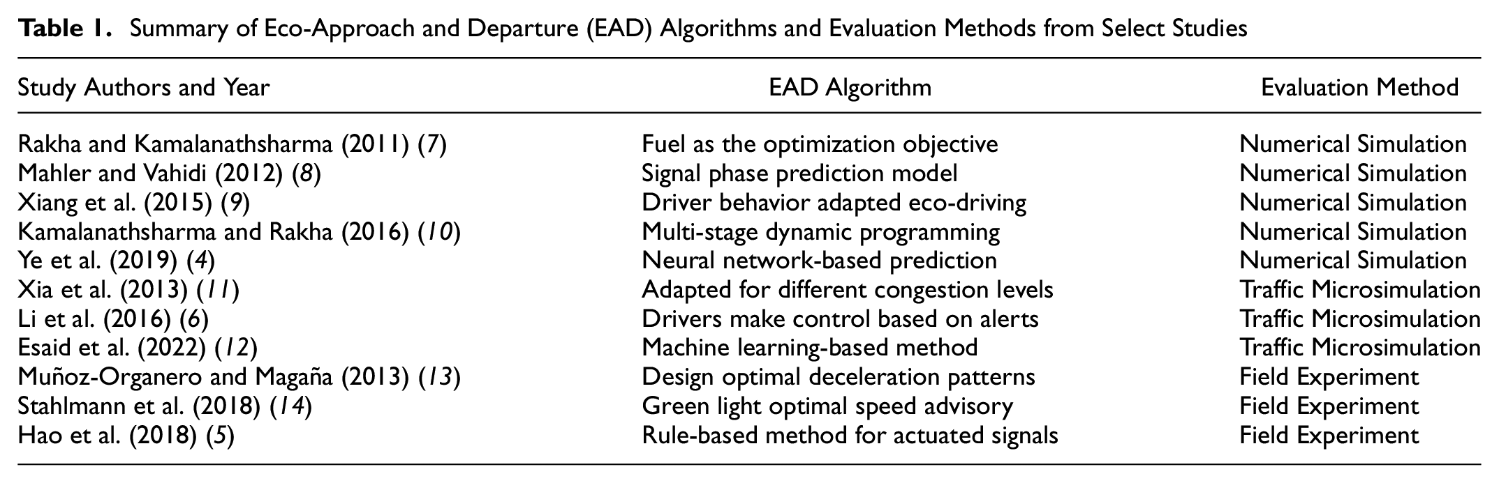
In the past decade, many studies have been conducted to evaluate the energy savings and emissions reduction potential of the EAD application under a variety of scenarios—from a simple scenario, such as fixed-time signals without traffic, to a more complex set-up that comprises actuated signals in different traffic conditions. Ye et al. ( 4 ) developed a prediction-based EAD strategy considering urban traffic and queues at intersections using the predicted states of the preceding vehicle. And the results from the numerical simulation show that the proposed EAD system could achieve 4.0% energy savings compared with a car-following baseline. Hao et al. ( 5 ) proposed an EAD system that was adaptive to the dynamic uncertainty for actuated signal and real-world traffic; real-world testing was conducted resulting in 6% energy savings. Li et al. ( 6 ) compared the safety, mobility, and environmental sustainability parameters of EAD-equipped vehicles versus non-equipped vehicles in a traffic microsimulation environment and achieved consistent mobility and environmental benefits in the EAD-equipped vehicles. Rakha et al. ( 7 ) used numerical simulations to show the importance of retaining microscopic fuel consumption models in the optimization function compared with using simplified objective functions. Mahler and Vahidi ( 8 ) used a signal phase prediction model to predict future SPaT status in an EAD application, which has shown increased energy efficiency in multi-signal numerical simulation. Xiang et al. ( 9 ) developed a closed-loop speed advisory model that is adaptive to the drivers’ behavior for eco-driving, showing a 4% fuel economy improvement compared with the baseline. Kamalanathsharma and Rakha ( 10 ) optimized the vehicles’ trajectories using the moving horizon dynamic programming approach, enhancing the computational efficiency using the A-star algorithm for real-time application. Xia et al. ( 11 ) proposed an enhanced EAD system considering both the SPaT information and the status of the preceding equipped vehicles using connected vehicle technology, which has shown higher benefits during higher levels of congestion. Esaid et al. ( 12 ) proposed a machine-learning trajectory planning algorithm that can achieve optimality and computational efficiency at the same time in multiple traffic microsimulation runs. Muñoz-Organero and Magaña ( 13 ) proposed an eco-driving assistant algorithm to reduce fuel consumption by calculating optimal deceleration patterns and minimizing the use of braking; the algorithm was tested with nine different drivers in five different models of vehicles. As shown in Table 1, all these studies used different methods in the evaluation of energy savings and emissions reduction benefits of EAD application, including numerical simulation, traffic microsimulation, or field experiment. Among the three types of method, numerical simulation ( 4 , 7 –10) is relatively easy to conduct, but it only simulates the EAD-equipped vehicle without consideration of other vehicles on the road. This limitation can be addressed by using traffic microsimulation ( 6 , 11 , 12 ) tools where different driving and traffic scenarios can be simulated to replicate real-world conditions. However, the evaluation of the EAD application using traffic microsimulation tools is complex and time-consuming, involving the coding, calibration, and validation of the simulation model as well as the implementation of EAD algorithms into the simulation model through an application programming interface. Lastly, the evaluation of the EAD application through field experiment ( 5 , 13 , 14 ) is expensive, and thus, is often conducted for a limited number of intersections and corridors. Meanwhile, the energy and emissions benefits of EAD depend heavily on intersection and corridor characteristics, such as the speed limit and the length of the road upstream of the intersection, and thus, the benefits of EAD measured at one intersection or corridor may not be applicable to others.

Table 1.

Summary of Eco-Approach and Departure (EAD) Algorithms and Evaluation Methods from Select Studies

Study Authors and Year	EAD Algorithm	Evaluation Method
Rakha and Kamalanathsharma (2011) ( 7 )	Fuel as the optimization objective	Numerical Simulation
Mahler and Vahidi (2012) ( 8 )	Signal phase prediction model	Numerical Simulation
Xiang et al. (2015) ( 9 )	Driver behavior adapted eco-driving	Numerical Simulation
Kamalanathsharma and Rakha (2016) ( 10 )	Multi-stage dynamic programming	Numerical Simulation
Ye et al. (2019) ( 4 )	Neural network-based prediction	Numerical Simulation
Xia et al. (2013) ( 11 )	Adapted for different congestion levels	Traffic Microsimulation
Li et al. (2016) ( 6 )	Drivers make control based on alerts	Traffic Microsimulation
Esaid et al. (2022) ( 12 )	Machine learning-based method	Traffic Microsimulation
Muñoz-Organero and Magaña (2013) ( 13 )	Design optimal deceleration patterns	Field Experiment
Stahlmann et al. (2018) ( 14 )	Green light optimal speed advisory	Field Experiment
Hao et al. (2018) ( 5 )	Rule-based method for actuated signals	Field Experiment

Over the past decade, extensive research has been focused on modeling vehicle energy consumption quantitatively, aiming to establish clear links between driving behavior, operational parameters, and energy use. Scholars have proposed various evaluation models to evaluate eco-driving capabilities, ranging from personalized time-series systems ( 15 ) that estimate future energy consumption to data-driven methods ( 16 ) that construct nonlinear relationships between driving behavior and energy use. Some models ( 17 ) use driving events as inputs, scoring eco-driving based on the occurrences of rapid acceleration or deceleration within a specific mileage. However, a common challenge arises in certain evaluation models that rely heavily on expert knowledge, introducing subjectivity into the assessment process. This reliance on expert opinions often complicates the construction of these models, affecting their overall objectivity. To achieve more objective assessments, researchers have explored indicators such as vehicle-specific power ( 18 ), energy consumed during braking ( 19 ), and positive kinetic energy ( 20 ) to construct an eco-driving evaluation model.

The objective of this research is to develop a model that can perform computationally efficient and practically feasible estimation of the energy saving potential of EAD. To achieve the research objective, a lookup table-based method is proposed where the lookup table stores the numerical relationships between vehicle energy consumption and key parameters in EAD operation, such as upstream and downstream link distance. These relationships replace the runtime computation in numerical simulation or traffic microsimulation with a faster array indexing operation. Similar methods ( 21 ) have been widely used in other research fields in view of the vast savings in processing time and the ability to store pre-calculated relationships for use in the execution of a model. Using the proposed method, one can quickly estimate the corridor-level or road network–level energy savings potential of the EAD application using only road length, speed limit, and travel time at each intersection as inputs. The estimation results can be used to select intersections for detailed evaluation in traffic microsimulation or prioritize intersections for field implementation. Note that our algorithm is not designed to fully replace traffic microsimulations or field tests since those methods are still more accurate, but to save time and narrow down the range of traffic signal selections. This can be seen as an assistant for the existing methods before they decide which intersections or corridors to simulate or conduct field tests. More specifically, the contributions of this research can be summarized as follows:

1) Efficient in computation: this research aims to create a computationally efficient model for estimating the energy savings potential of Eco-Approach and Departure (EAD). The model seeks practical feasibility while minimizing computational load.

2) Cost-effective in data collection: the inputs to this estimation model only consist of road length, speed limits, and intersection travel times, which are cost and effort effective to acquire and process.

3) Complementary to established methods: the estimation outcomes serve as a basis for selecting intersections for in-depth evaluation within traffic microsimulations or for prioritizing intersections for potential field implementation. This research would help identify the target intersection for deployment in the preliminary stages of decision making.

To develop the estimation method, data generated from an extensive traffic microsimulation of an EAD application for heavy-duty trucks on real-world corridors in Carson, California, were used. First, two lookup tables (one for the baseline scenario and the other for the EAD scenario) were created that compiled upstream distance, downstream distance, average travel time, and energy consumption for the individual intersections. Then, each lookup table was used to build an estimation model, which was later calibrated based on the ratio between the actual and estimated energy consumption. Using the calibrated models, the energy consumption for both the baseline and EAD scenarios at each intersection can be estimated, and subsequently, the energy savings can be calculated.

Methodology

In this section, we will discuss the microsimulation-based approach for estimating the energy saving potential. We will describe the system architecture, including four key components: scenario generation, online EAD system, offline EAD system, and energy benefit estimation model. The EAD application for heavy-duty trucks, including the online and offline EAD system, was previously developed and implemented in the traffic microsimulation models of four real-world trucking corridors in Carson, California, to evaluate the energy saving potential of EAD for trucking applications ( 22 ). In this paper, we extend the work to the upstream and downstream to design, calibrate, and validate the lookup table-based energy consumption estimation method using data generated from the traffic microsimulation models.

System Architecture

As shown in Figure 1, the proposed system has four major components: scenario generation, online EAD system, offline EAD system, and energy benefit estimation model. The scenario generation step initializes the system with a well-calibrated simulation network. A signalized intersection with 1,500 m upstream and downstream links were created to cover all the potential upstream and downstream distance scenarios for the EAD problem. We then test the baseline and EAD cases for 1,000 runs respectively to create a sufficient data pool to evaluate the energy saving potential under various road, traffic, and signal conditions.

Figure 1.

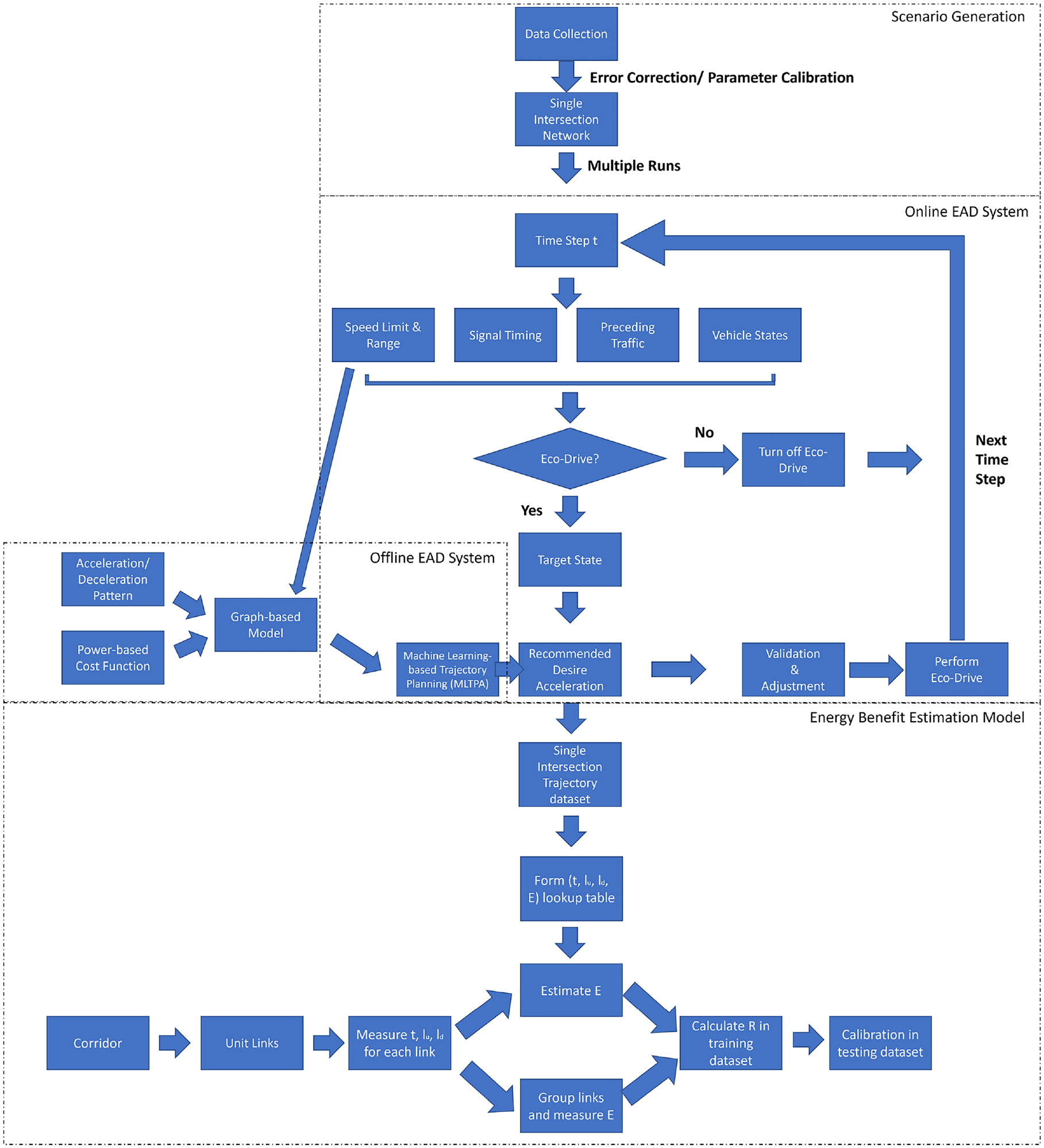
System diagram of the Eco-Approach and Departure (EAD) application.

The EAD system consists of online and offline systems. The offline EAD system trains a machine learning-based trajectory planning model, which was then used in the online EAD system to output the suggested speed and acceleration profile for the host vehicle in real time. In the offline system, a graph-based trajectory planning model is first developed based on the unique powertrain characteristics and vehicle dynamics of trucks. This graph model creates a data set of input-output pairs using different combination inputs of the truck speed, location, and signal states to output the optimal acceleration. To save computational time while maintaining high accuracy, a machine learning-based trajectory planning model is then trained using the input-output data set so that the online EAD system can give the most eco-friendly speed suggestion in real time ( 12 ). The proposed machine-learning trajectory planning algorithm (MLTPA) is designed to enable real-time optimization. The approach involves training a random forest model to emulate the solution derived from an existing optimization method known as the graph-based trajectory planning algorithm (GBTPA). By adopting the proposed MLTPA, one can significantly reduce computation time from tens of seconds to just a few milliseconds. Simulation results demonstrate that MLTPA consistently achieves a median improvement in energy savings ranging from 5.0% to 6.20% across multiple simulation runs. This approach also exhibits the potential to approximate various other trajectory planning algorithms, ensuring real-time performance without compromising optimality. More technical details can be found in Esaid et al. ( 12 ).

In the online system, at each time step, different sources of information are inputs to form a safe and energy-saving target speed. Given the current signal states and location of the vehicle, the system will evaluate whether the vehicle can pass the intersection in the current phase. And given the states of the preceding vehicle, the system will also decide whether the host vehicle will be blocked by the front vehicle. If such safety requirements are not satisfied, the EAD system will shut down and the system will give control back to the default controller in the simulation software. If all the safety requirements are satisfied, the vehicle states will be fed into the trained machine-learning model to output the desired acceleration and speed ( 22 ). While implementing the online EAD system, we track the entire exact speed profile of all the baseline and EAD trucks no matter if they are driven under the EAD algorithm or the default controller in the simulation engine. These speed profile data outputs from the simulation will reflect how the EAD system performs in the traffic and will form a lookup table for the energy benefit estimation model.

With the well-calibrated single-intersection microsimulation network and real-time online EAD model, the single-intersection trajectory data sets and lookup tables are generated using multiple runs to feed into the energy benefit estimation model. In this model, a corridor or network is first divided into multiple unit links. Then, the energy consumption for each time (t), upstream distance (l_u), and downstream distance (l_d) combination is measured. Next, the adjustment factor R is calculated based on the actual energy consumption and the estimated energy using the lookup table. And this factor will be applied to the test data set for energy estimation. Note that the “actual” energy consumption is defined as the simulated energy consumption for both baseline and eco-driving. The “actual” is mentioned to compare with the estimated energy consumption derived from the uncalibrated lookup table. The detail of each step in the model will be discussed in the next section.

Energy Benefit Estimation Model

Unit Intersection Lookup Table

Many parameters are related to energy consumption in the proposed EAD model, for example, starting and ending locations with respect to the intersection, the SPaT information, the speed limit, the traffic condition, and so forth. The upstream distance (l_u) determines the maximum distance of which the eco-driving could be initiated. If l_u is smaller than the communication range of the connected signal, the host vehicle will start eco-driving as soon as it enters the intersection. Otherwise, the host vehicle will drive without connection until it enters the communication range. The second parameter that is important in the EAD model is the downstream distance (l_d), which describes how far the vehicle could drive after passing the intersection. l_d constrains the target speed the vehicle could reach at the end of the network, therefore affecting the energy consumption of the model. Both distance measures are critical in the EAD model and are convenient to acquire from the geographic database. The speed and time-related parameters are also significant in the EAD process. For example, when the traffic is congested, the eco-driving will not be able to be effectively performed because of the close gap between the host vehicle and the leading vehicle. When the traffic signal has a longer red-light phase, the host vehicle will be more likely to slow down because of the signal and queue. When the city engineers are estimating potential energy benefits by enabling certain connected signals, we would like to expect high efficiency and accuracy in this process. Although all these parameters are important in estimating the energy consumption, we only choose the travel times along with upstream/downstream distances in the lookup table as they are easier to measure and obtain. Other parameters, such as the traffic signal timing and traffic condition, are difficult to acquire or estimate in a real-time manner.

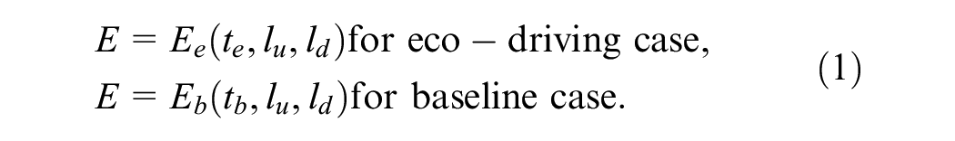
We create two lookup tables (one for baseline and one for eco-driving) where the energy consumption (E) for each (t, l_u, l_d) combination in the single-intersection simulation was listed. The two lookup tables can be summarized as two functions below:

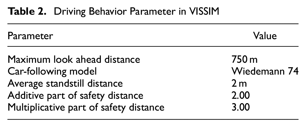
\begin{matrix} E = E_{e} (t_{e}, l_{u}, l_{d}) for eco - driving case, \\ E = E_{b} (t_{b}, l_{u}, l_{d}) for baseline case . \end{matrix}

(1)

As part of the energy benefit estimation model, the single-intersection simulation provides the simplest EAD scenario, from which different (t, l_u, l_d) combinations could be extracted. The simulations are conducted with both eco-driving and baseline algorithms for a total of 1,000 runs each. Between each run of eco-driving and baseline, the initial conditions are set to be the same using the same random seed number. The large number of runs guarantees that a sufficient data pool could be created to evaluate the energy savings. The baseline algorithm is the default VISSIM driving model with parameters shown in Table 2. The energy consumption for each run is fed into the lookup table corresponding to the three indicator values. In the case where the same indicator values are reached among multiple runs, the energy consumption will be the average value between them. Later, the corridor with multiple intersections could be split into single intersections, calculated separately, and added together for total energy consumption and benefit estimation.

Table 2.

Driving Behavior Parameter in VISSIM

Parameter	Value
Maximum look ahead distance	750 m
Car-following model	Wiedemann 74
Average standstill distance	2 m
Additive part of safety distance	2.00
Multiplicative part of safety distance	3.00

Lookup Table Calibration

The lookup table in the previous step is obtained by running microsimulations of a single-intersection network. The network is designed to have large enough l_u and l_d (both 1,500 m) so that the lookup table could cover all conditions of the real-world intersections. However, such a lookup table might not work when the network is extended to corridors of multiple intersections with different lengths of l_u and l_d, especially when the intersections are closely spaced. When the l_u or l_d is small, vehicles usually prepare to decelerate before they reach the desired speed, causing a smaller average speed and longer travel time. The actual energy consumption is usually less than the estimated value from E_e or E_b. In urban areas where higher traffic densities and more complex road networks are often seen, distances between intersections are sometimes close, leading to shorter EAD optimizable distances and larger gaps between actual and estimated energy consumption. Rural areas typically experience lower traffic density and fewer intersections. EAD driving can maintain a longer time at steady speeds to minimize unnecessary acceleration and deceleration, leading to similar actual and estimated energy consumption. Therefore, the R factor is close to one when the link distance is long and gets smaller when the link distance is short.

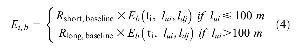
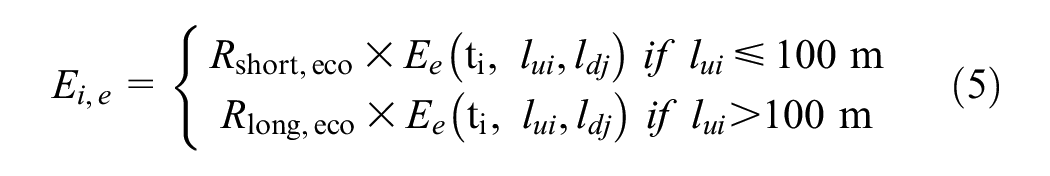
To calibrate the adjustment factor R (defined as the ratio between the actual energy and the estimation), we first used corridor simulation data from two corridors as training sets and collected actual energy consumption data for each link. We then estimate the energy consumption at corresponding links from the single-intersection simulation data set. According to the link distance (short or long) and driving mode (eco-drive or baseline), data were categorized into four groups. Here, short links are defined as links in which l_u ≤ 100 m, and long upstream links are defined as links in which l_u > 100 m. The adjustment factor R between actual and estimation for certain link length types and driving modes is then calculated as below:

R = \frac{\sum_{i = 1}^{k} E_{actua l_{i}}}{\sum_{i = 1}^{k} E_{estimatio n_{i}}}

(2)

where k is defined as the number of signals with the same link length type and driving mode. $R$ could be more accurate with a finer classification of the link distances. But since our data is limited, more link distance groups will result in fewer data for each group and make it harder to calibrate. Based on the amount of data available and the accuracy of the results, we have chosen these four groups of adjustment factors.

Scenario and Input Identification

For any given corridor or network, the first step in this approach is link division. We define the link length d_ij as the distance between the stop line of the upstream intersection i and downstream intersection j, downstream distance of intersection i (defined as l_di) and upstream distance of intersection j (defined as l_uj) are then defined below:

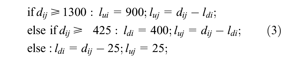
\begin{matrix} if d_{ij} \geq 1300 : l_{ui} = 900; l_{uj} = d_{ij} - l_{di}; \\ else if d_{ij} \geq 425 : l_{di} = 400; l_{uj} = d_{ij} - l_{di}; \\ else : l_{di} = d_{ij} - 25; l_{uj} = 25; \end{matrix}

(3)

The main idea of choosing the threshold values of the link distances is to keep the downstream distance of at least 400 m when the distance between two intersections is larger than 425 m. And when the distance between two intersections is shorter than 425 m, we want to keep the downstream distance as large as possible. This is to ensure that the vehicle could reach the speed limit after passing the intersection so that the energy difference between eco-drive and baseline is solely dependent on the approaching section of the driving. For a heavy-duty truck driving on a road with a speed limit of 45 mph (20 m/s) with an average acceleration of 0.5 m/s², the distance it takes to reach the speed limit from rest is 400 m.

The baseline travel time for each link can be either derived from sample truck trajectory data, estimated by the equations in the Highway Capacity Manual (HCM) or looked up from the historical travel time in Google Map Application Programming Interface (API). HCM provides the estimated travel speed based on a series of numerical equations. The parameter values in the model depend on the signal timing parameters, street category, and so forth. Also, the HCM model requires a large amount of data ( 23 ). Compared with HCM, Google Map API provides the estimated travel speed based on the current traffic condition and the historical travel time of similar periods, without the need for heavy computation. Since obtaining the parameters of certain intersections could be time-consuming, Google Map API is ideal and was used in Section 3.3. Since the link travel times for eco-drive scenarios are similar to corresponding baseline cases, we used the same travel time for both baseline and eco-driving on the same network. For baseline scenarios, all the intersections are non-connected. For eco-drive scenarios, intersections can be connected or non-connected, according to the implementation plan.

Energy Benefit Estimation

For each link in the real-world corridor, the estimated energy consumption under the baseline scenario is

E_{i, b} = {\begin{matrix} R_{short, baseline} \times E_{b} (t_{i}, l_{ui}, l_{dj}) if l_{ui} \leq 100 m \\ R_{long, baseline} \times E_{b} (t_{i}, l_{ui}, l_{dj}) if l_{ui} > 100 m \end{matrix}

(4)

where R is calculated from Step 2 using the grouped training data. The equations above are also applicable to the links with non-connected signals for eco-drive scenarios. For links with connected signals, the estimated energy consumption under the eco-drive scenario is

E_{i, e} = {\begin{matrix} R_{short, eco} \times E_{e} (t_{i}, l_{ui}, l_{dj}) if l_{ui} \leq 100 m \\ R_{long, eco} \times E_{e} (t_{i}, l_{ui}, l_{dj}) if l_{ui} > 100 m \end{matrix}

(5)

After calculating the energy consumption of single intersections of a corridor, the total baseline energy consumption is the summation of all the calibrated energy values, and the energy benefit is then calculated correspondingly.

E_{total} = \sum_{i = 1}^{n} E_{i}

(6)

E_{saving} = 1 - \frac{E_{total, e}}{E_{total, b}}

(7)

Numerical Experiments

In this section, we first show the results of the unit intersection simulation. Then, we validate the proposed estimation method using the traffic microsimulation-generated data from four real-world corridors in Carson, California. Lastly, the validated models are applied to estimate the potential energy savings from the EAD application for the entire truck route network in the city of Carson.

Unit Intersection Simulation

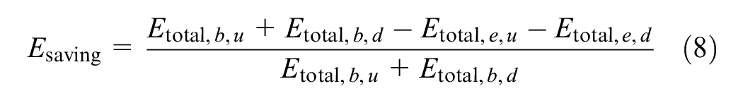
As mentioned in the methodology section, a single-intersection simulation network with 1,500 m l_u and l_d was built in VISSIM to create the lookup table of the energy consumption correspondence. After building the unit intersection network, 1,000 runs for baseline case and 1,000 runs for eco-driving were conducted to create the required database for the lookup table, and the total process took less than 3 h. To understand the impact of each parameter on the performance of the EAD algorithm, we plot the energy consumption v.s. l_u and l_d when travel time is set to be 100 s, as shown in Figure 2. As can be seen from Figure 2b, when l_d and t are constant, the total energy consumption decreases as l_u increases. This is because the vehicle tends to slow down before the intersection and accelerate after passing the intersection when l_u is small, causing extra energy consumption in the acceleration process. We can also see that when l_u and t are constant, the total energy consumption increases as l_d increases. This is because the host vehicle spends more time accelerating to coasting speed when l_d increases. As for energy benefit, E_saving ranges from 0% to 30%, increases as l_u increases and decreases as l_d increases. To explain this phenomenon, we can interpret E_saving using the formula below:

E_{saving} = \frac{E_{total, b, u} + E_{total, b, d} - E_{total, e, u} - E_{total, e, d}}{E_{total, b, u} + E_{total, b, d}}

(8)

where $E_{total, b, u}$ represents the total energy consumption for baseline in the upstream driving. When l_u increases, the host vehicle can start eco-driving at an earlier stage, causing $E_{total, b, u} - E_{total, e, u}$ to increase while keeping $E_{total, b, d} - E_{total, e, d}$ consistent, therefore $E_{saving}$ increases. Once the vehicle passes the intersection, the V2I communication will terminate and the connected vehicle will perform the same as the baseline vehicle. When l_d increases, the numerator of formula 9 remains unchanged while $E_{total, b, d}$ increases, therefore $E_{saving}$ decreases.

Figure 2.

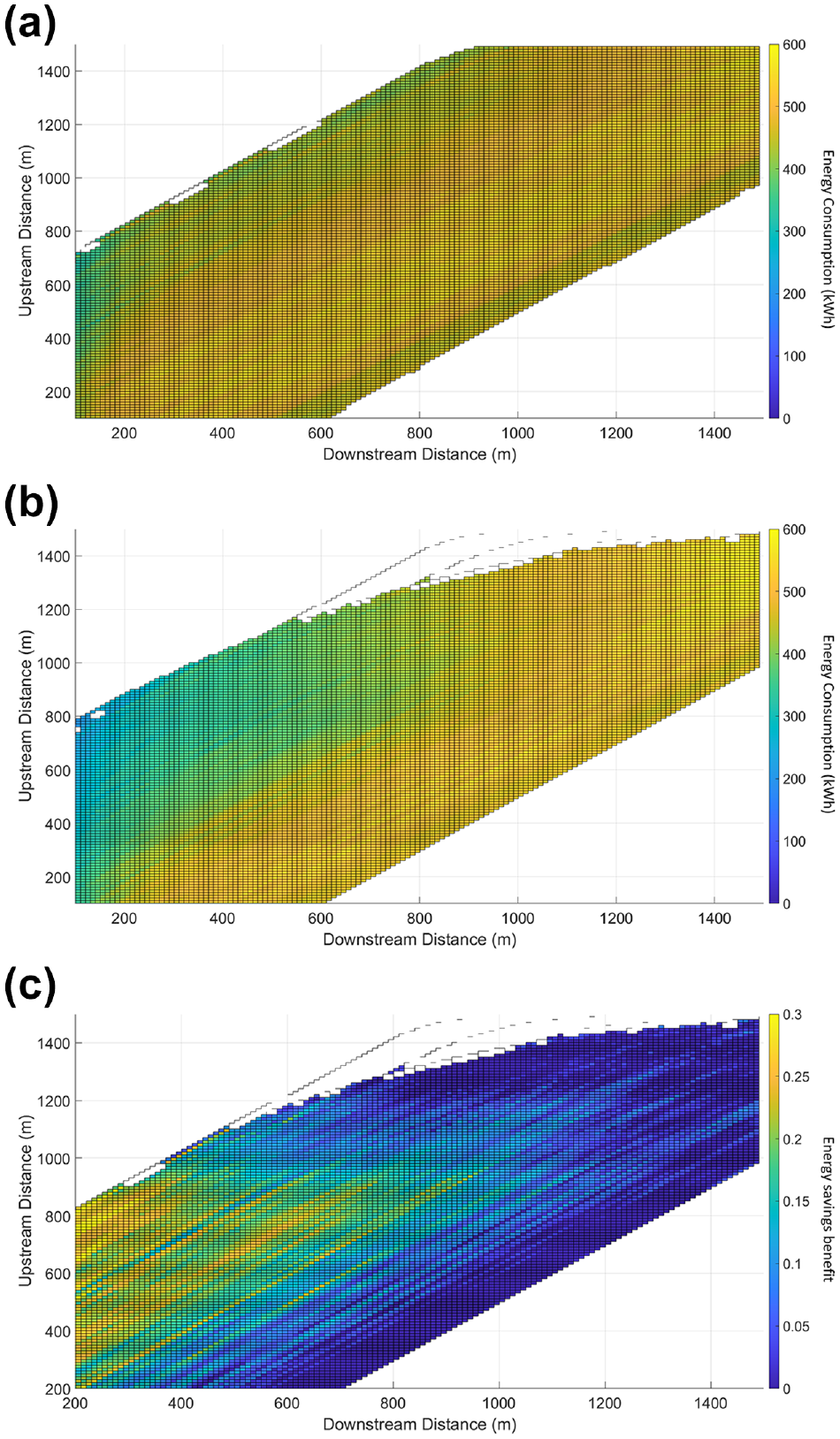
Energy consumption and energy benefit for t = 100 s: (a) energy consumption for baseline; (b) energy consumption for Eco-Approach and Departure (EAD); and (c) energy savings benefit (energy for baseline − energy for EAD)/energy for baseline).

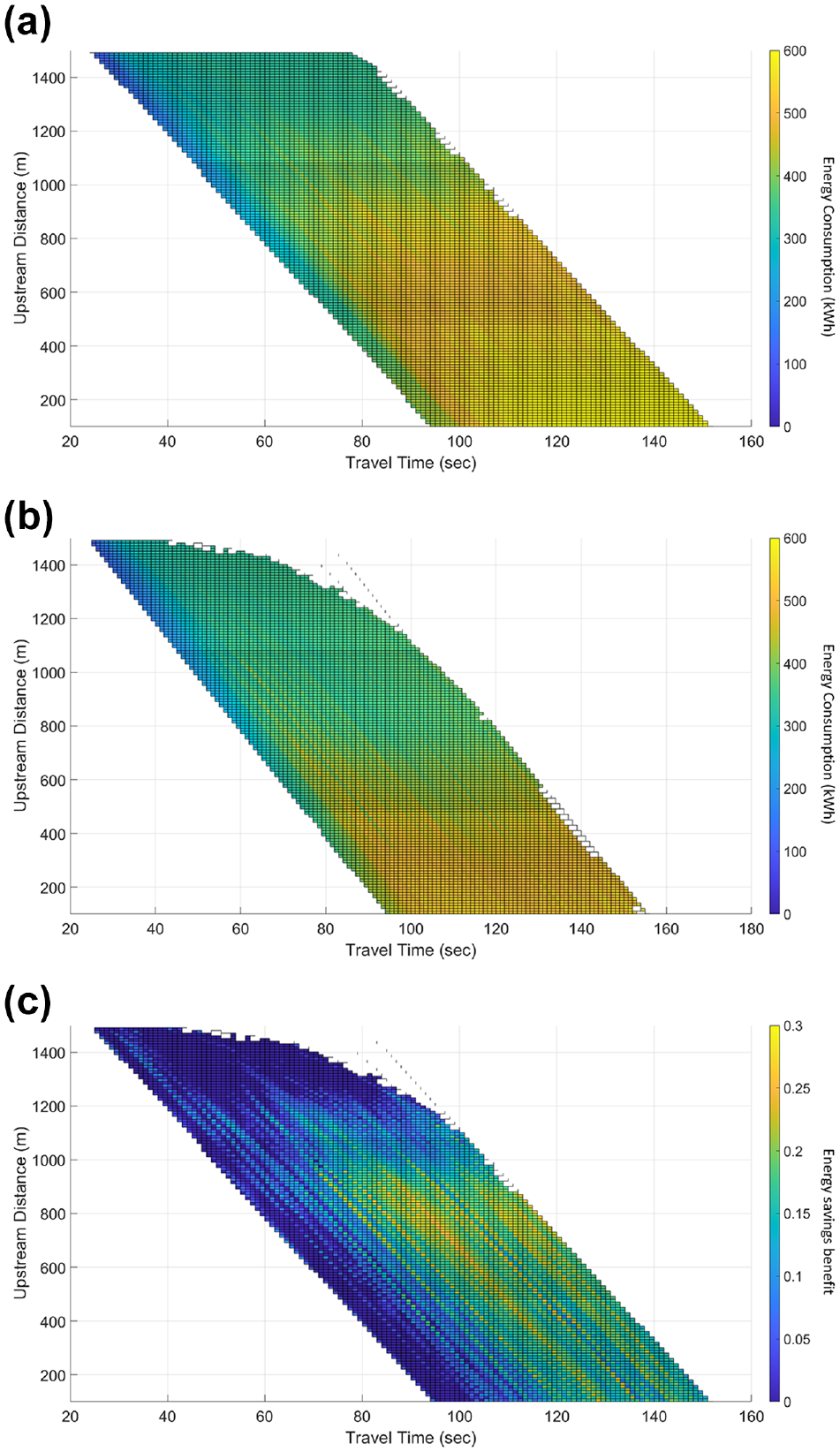
Next, we plot the energy consumption v.s. l_u and t when l_d is set to be 500 m, in Figure 3. As can be seen from Figure 3, a and b , when l_d and t is constant, $E_{total, e}$ decreases as l_u increases, which is similar to Figure 2. When l_d and l_u is constant, as t increases, $E_{total, e}$ increases to a certain threshold before reaching constant. This is because when t is smaller than the threshold, the vehicle will spend less time decelerating and accelerating. When t is larger than the threshold, all the vehicles will have to stop at the intersection, therefore costing the same $E_{total, e}$ for proceeding a similar speed profile downstream.

Figure 3.

Energy consumption and energy benefit for l_d = 500 m: (a) energy consumption for baseline; (b) energy consumption for Eco-Approach and Departure (EAD); (c) energy savings benefit (energy for baseline − energy for EAD/energy for baseline).

Corridor Energy Benefit Estimation

In the simulation scenario, we created a data set for the single-intersection simulation and estimated the raw energy consumption for each link in the four corridors, namely Wilmington North (WN), Wilmington South (WS), Alameda North (AN), and Alameda South (AS), as shown in Figure 4. The four corridors are located right next to the Port of Los Angeles and Port of Long Beach, the two busiest container ports in the United States. There are 11 and eight signals in the Wilmington S/N and Alameda S/N corridors respectively, and each corridor has five connected signals as labeled in the figure. Similar to Hao et al. ( 22 ), we adapted the signal timing and traffic conditions from the real world and created a simulation environment in VISSIM. The heavy-duty truck defined in the simulation was set to have a weight of 18,000 kg. The average acceleration and deceleration profile of the heavy-duty truck is calibrated with real-world data and some of the key parameters of the driving behavior are defined in Table 2.

Figure 4.

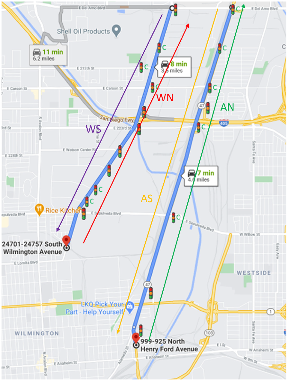
Location of four corridors (AN, AS, WN, WS) applied in the simulation. Each corridor is highlighted in different colors.

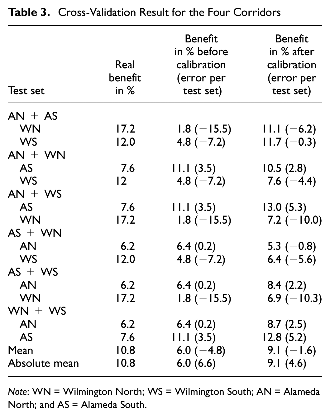
The baseline is controlled by VISSIM using the default driver model, and the eco-driving data is created using the EAD model mentioned in the background section. We employed an exhaustive cross-validation technique called leave-p-out cross-validation ( 24 ) with p = 2. This involved using data from two corridors as the training set and validating the trained model against data from the remaining two corridors. The validation was repeated for all possible ways of splitting the training versus the validation set. The result is shown in Table 3.

Table 3.

Cross-Validation Result for the Four Corridors

Test set	Real benefit in %	Benefit in % before calibration (error per test set)	Benefit in % after calibration (error per test set)
AN + AS
WN	17.2	1.8 (−15.5)	11.1 (−6.2)
WS	12.0	4.8 (−7.2)	11.7 (−0.3)
AN + WN
AS	7.6	11.1 (3.5)	10.5 (2.8)
WS	12	4.8 (−7.2)	7.6 (−4.4)
AN + WS
AS	7.6	11.1 (3.5)	13.0 (5.3)
WN	17.2	1.8 (−15.5)	7.2 (−10.0)
AS + WN
AN	6.2	6.4 (0.2)	5.3 (−0.8)
WS	12.0	4.8 (−7.2)	6.4 (−5.6)
AS + WS
AN	6.2	6.4 (0.2)	8.4 (2.2)
WN	17.2	1.8 (−15.5)	6.9 (−10.3)
WN + WS
AN	6.2	6.4 (0.2)	8.7 (2.5)
AS	7.6	11.1 (3.5)	12.8 (5.2)
Mean	10.8	6.0 (−4.8)	9.1 (−1.6)
Absolute mean	10.8	6.0 (6.6)	9.1 (4.6)

Note: WN = Wilmington North; WS = Wilmington South; AN = Alameda North; and AS = Alameda South.

The validation results show that the real energy benefits range from 6.2% to 17.2% with an average value of 10.8%. The estimation error after calibration ranges from −10.3% to +5.3% with an average value of 9.1% and a mean absolute error of 4.6% per test set. Compared with the energy benefit (6.0%) and absolute error per test set (6.6%) before calibration, both values showed a noticeable improvement after calibration. More specifically, five out of six validation trials show a significantly better estimation result after the calibration factor is applied. The raw estimated energy turns out to be an overestimation for all data sets, which might be caused by the lower traffic and higher average speed in the corridor simulation compared with the single-intersection simulation. The proposed method can also make an accurate estimation for the energy consumption in both baseline and eco-driving with less than 10% estimation error. Throughout the process from unit intersection simulations to energy benefit estimations, the majority of time is consumed on conducting all the baseline and eco-drive runs at the training phase. Once the simulations are completed, the lookup table-based energy estimation approach only takes less than 1 s of computational time for each corridor. Therefore, the proposed method is efficient in time and effort for city-level or regional-level implementations.

City of Carson Truck Route Energy Benefit Estimation

We then applied the energy benefit estimation model to the truck route network in the city of Carson and estimated the potential energy savings using the EAD application. Figure 5 shows the truck routes and parking map in Carson, California, where 14 east–west and 10 north–south corridors are colored in yellow. To estimate the energy consumption and benefit for the corridors, we need to divide each corridor into links based on the traffic signals and calculate the travel time and upstream/downstream length for each link. In Google Earth (Figure 6), we locate all the traffic signals with their length on the corridor and note down the longitude and latitude of the beginning and end of each corridor. Using Google Map Distance Matrix API, we collect the real-time travel time data of the entire corridor using the longitude and latitude coordinates of the corridor. To adapt to the uncertain traffic conditions on the corridors, travel time data are collected every 15 mins for seven days and then averaged into hourly data. Finally, the link travel time $t_{L_{i}}$ is calculated using the corridor travel time $t_{c}$ based on the speed limit $v_{L_{i}}$ and the distance of each link $d_{i}$ , shown as below:

t_{L_{i}} = t_{c} \times \frac{\frac{d_{i}}{v_{L_{i}}}}{\sum_{j = 1}^{n} \sum \frac{d_{j}}{v_{L_{j}}}}

(9)

While the distance matrix API only provides a general travel time for all the vehicles, since we are applying the algorithm to local corridors with a speed limit between 35 and 45 mph, we assume the truck travel speed is close to the general traffic speed estimated from the API. With the travel time, distance, and the calibration factor calculated from the simulation study, the estimated energy consumption and EAD estimation are listed in Table 4 below. Note that some corridors with no traffic signal have been removed from the table.

Figure 5.

Truck route and parking map in the city of Carson. The corridor highlighted with a dashed green line is Figueroa St.

Figure 6.

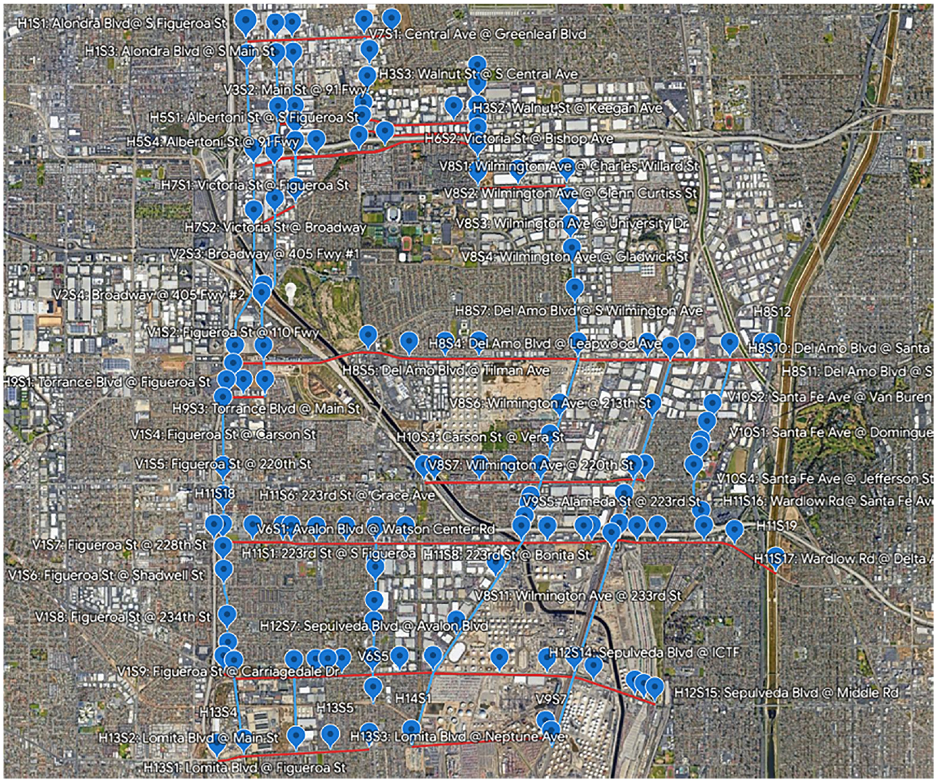
East–west (red) and north–south (blue) corridors in the city of Carson from Google Earth.

Table 4.

Truck Route Energy Consumption and Saving

	Name	Corridor length (mi)	# Signals	Baseline energy (kWh)	Eco-driving energy (kWh)	Energy savings (%)
Horizontal
1	Alondra Blvd	1.2	8	3.6	2.9	−19
3	E Walnut St	1.0	4	2.2	1.7	−25
5	Albertoni St	1.1	10	3.6	3.3	−9
6	E Victoria St	0.7	4	1.6	1.3	−20
7	W Victoria St	0.4	4	1.5	1.5	−1
8	Del Amo Blvd	4.5	21	9.6	9.2	−4
9	W Torrence Blvd	0.3	4	1.2	1.2	−5
10	E Carson St	1.9	10	5.1	4.2	−17
11	223rd St	4.8	30	14.2	12.5	−12
12	Sepulveda Blvd	3.7	28	8.8	8.0	−9
13	Lomita Blvd	1.3	6	4.0	3.5	−11
Vertical
1	S Figueroa St	6.1	32	15.6	13.5	−14
2	S Broadway	3.0	14	8.4	6.7	−20
3	S Main St (north)	1.4	8	3.9	3.1	−20
5	S Avalon Blvd (north)	1.0	10	3.5	2.9	−16
6	S Avalon Blvd (south)	1.4	11	4.1	3.5	−17
7	S Central Ave	0.7	11	3.1	2.6	−16
8	S Wilmington Ave	5.1	31	15.6	13.6	−13
9	Alameda St	3.4	11	8.4	7.0	−17
10	Santa Fe Ave	1.5	12	4.5	3.5	−23

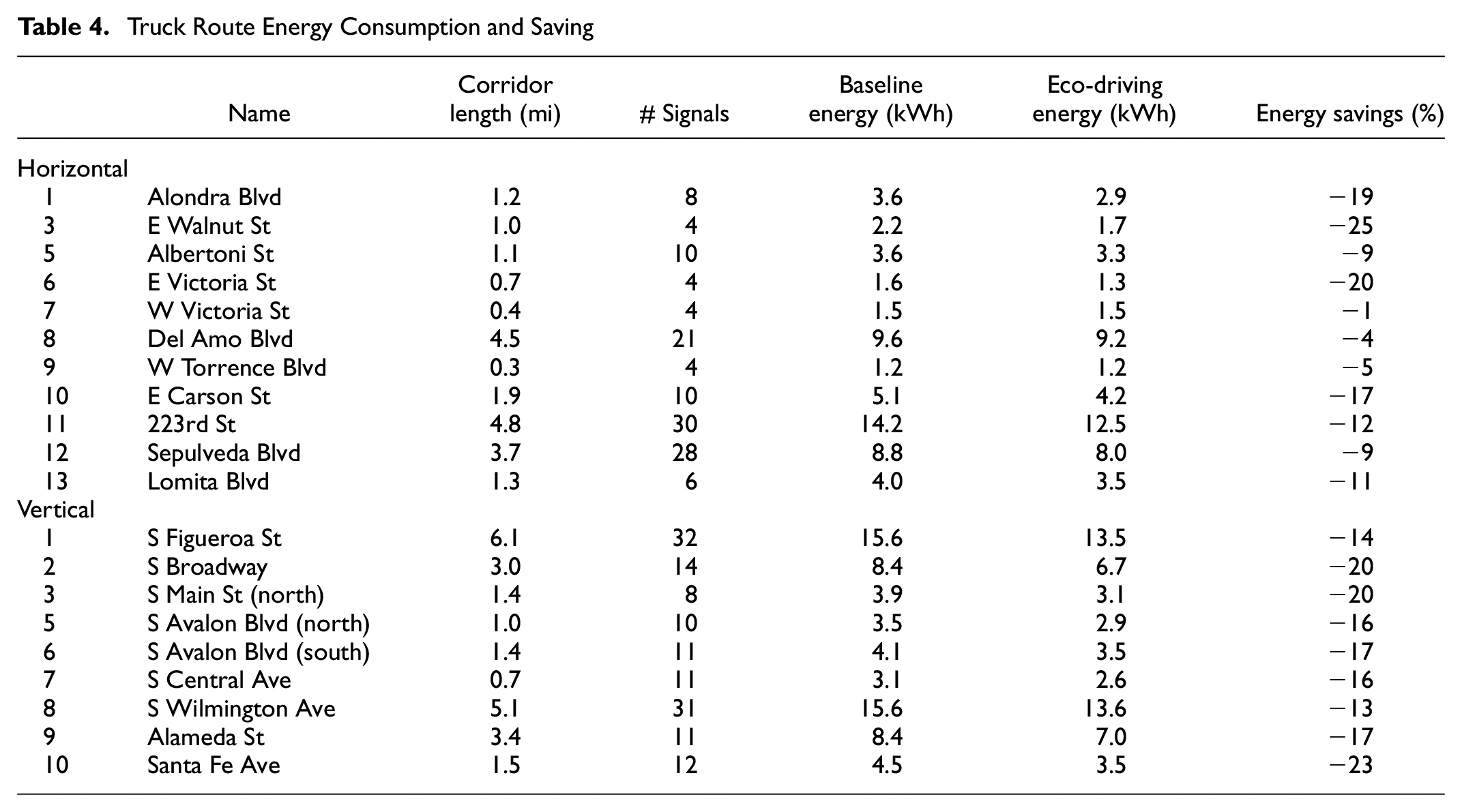
The results show that the potential energy savings vary by the characteristic of each corridor, ranging from 1% to 25% with an average of 14%. In general, the corridor with closely spaced intersections (≤0.1 mi on average, for example, W Victoria St and W Torrence Blvd) has less energy saving than the rest of the intersections. The baseline vehicles in sparsely spaced intersections may need to accelerate to high speed before reaching the next intersection, which provides optimization space for the EAD algorithm to control the acceleration process to avoid a stop in the next intersection. On the other hand, the baseline vehicles in closely spaced intersections do not need to accelerate to a high speed before reaching the next intersection, so the performance of the EAD algorithm in this case is less effective.

With regard to the average speed (or travel time), the eco-driving strategy shows less energy saving when the average speed is very high (most vehicles in free flow) or low (heavy congestion with over-saturation), and is more effective when the average speed is in the middle, where vehicles have proper motivation and space to perform the EAD algorithm at intersections.

Conclusion

This paper presents a computationally efficient and practically feasible methodology for evaluating and estimating the potential energy savings of using EAD along trucking corridors within cities. Using the road length, travel time, and speed limit at each intersection in the corridor, one can quickly estimate the corridor-level energy savings with customized connected or non-connected signal combinations with high accuracy. We validated the proposed estimation method using the traffic microsimulation-generated data from four real-world corridors in Carson, California. The proposed method made an accurate estimation of the energy consumption in both the baseline and eco-driving cases with less than 10% estimation error, and the cross-validation results showed that the benefit estimation error ranges from −10% to +5% with a mean error of −1.6% and a mean absolute error of 4.6%. This method could support city planners and engineers to estimate potential energy benefits when enabling certain connected signals and to decide which signals to prioritize for enabling connectivity.

In our future work, we plan to apply the proposed methodology to different types of vehicle and roadway network. Since the current analysis mostly relies on four corridors, additional simulations will be performed to estimate the energy saving benefits with new simulation networks and under different connected vehicle penetration rates. Also, the estimation result could be more accurate with more test data and a finer classification of the link distances. And creating further simulation networks for the truck routes in the city of Carson would help validate the accuracy of the proposed algorithm. Real-world field tests will also be conducted to verify and improve the proposed algorithm.

Footnotes

Acknowledgements

The authors would like to acknowledge California Energy Commission and Los Angeles County Metropolitan Transportation Authority for providing co-funding, as well as Los Angeles County Department of Public Works, city of Carson, City of Los Angeles Department of Transportation, Econolite, McCain, and Western Systems for their technical support. We gratefully acknowledge the contributions of Pascal Amar, Kyle Palmeter, and Stephen Orens to this research, who conducted the work during their tenure at Volvo Group.

Author Contributions

The authors confirm contribution to the paper as follows: study conception and design: Kanok Boriboonsomsin, Peng Hao, Aravind Kailas, Pascal Amar, Matthew Barth; data collection: Zhensong Wei, Kyle Palmeter, Lennard Levin, Stephen Orens; analysis and interpretation of results: Zhensong Wei, Peng Hao, Kanok Boriboonsomsin; draft manuscript preparation: Zhensong Wei, Peng Hao, Kanok Boriboonsomsin, Aravind Kailas. All authors reviewed the results and approved the final version of the manuscript.

Declaration of Conflicting Interests

The author(s) declared no potential conflicts of interest with respect to the research, authorship, and/or publication of this article.

Funding

The author(s) disclosed receipt of the following financial support for the research, authorship, and/or publication of this article: This paper was prepared as a result of work sponsored by California Air Resources Board. The California Collaborative Advanced Technology Drayage Truck Demonstration Project is part of California Climate Investments, a statewide program that puts billions of Cap-and-Trade dollars to work reducing greenhouse gas emissions, strengthening the economy, and improving public health and the environment—particularly in disadvantaged communities. Funding was also provided by South Coast Air Quality Management District’s Clean Fuels Program, which since 1988 has provided over $320 million, leveraging $1.2 billion, to fund projects to accelerate the demonstration and deployment of clean fuels and transportation technologies through public-private partnerships.

ORCID iDs

Zhensong Wei

Aravind Kailas

Kyle Palmeter

Lennard Levin

Stephen Orens

Matthew Barth

Kanok Boriboonsomsin

The opinions, findings, conclusions, and recommendations are those of the authors and do not necessarily represent the views of project sponsors or other team members.

References

Inventory of U.S. Greenhouse Gas Emissions and Sinks. www.epa.gov/sites/production/files/2020-04/documents/us-ghg-inventory-2020-main-text.pdf.

Morrow

W. R.

Gallagher

K. S.

Collantes

Lee

Analysis of Policies to Reduce Oil Consumption and Greenhouse-Gas Emissions from the US Transportation Sector. Energy Policy, Vol. 38, No. 3, 2010, pp. 1305–1320.

CV Pilot Deployment Program. www.its.dot.gov/pilots/pilots_environment.htm.

Hao

Boriboonsomsin

Barth

M. J.

Prediction-Based Eco-Approach and Departure at Signalized Intersections with Speed Forecasting on Preceding Vehicles. IEEE Transactions on Intelligent Transportation Systems, No. 20, No. 4, 2019, pp. 1378–1389.

Hao

Boriboonsomsin

Barth

M. J.

Eco-Approach and Departure (EAD) Application for Actuated Signals in Real-World Traffic. IEEE Transactions on Intelligent Transportation Systems, Vol. 20, No. 1, 2018, pp. 30–40.

Barth

M. J.

Zhang

Safety, Mobility and Environmental Sustainability of Eco-Approach and Departure Application at Signalized Intersections: A Simulation Study. Proc., IEEE Intelligent Vehicles Symposium (IV), Gothenburg, Sweden, 19–22 June, 2016, IEEE, New York, pp. 1109–1114.

Rakha

Kamalanathsharma

R. K.

Eco-Driving at Signalized Intersections Using V2I Communication. Proc., 14th International IEEE Conference on Intelligent Transportation Systems (ITSC), Washington, D.C., 5–7 October, 2011, IEEE, New York, pp. 341–346.

Mahler

Vahidi

Reducing Idling at Red Lights Based on Probabilistic Prediction of Traffic Signal Timings. Proc., American Control Conference (ACC), Montreal, Canada, 27–29 June, 2012, IEEE, New York, pp. 6557–6562.

Xiang

Zhou

Zhang

W.-B.

Qin

Mao

A Closed-Loop Speed Advisory Model with Driver’s Behavior Adaptability for Eco-Driving. IEEE Transactions on Intelligent Transportation Systems, Vol. 16, No. 6, 2015, pp. 3313–3324.

10.

Kamalanathsharma

R. K.

Rakha

H. A.

Leveraging Connected Vehicle Technology and Telematics to Enhance Vehicle Fuel Efficiency in the Vicinity of Signalized Intersections. Journal of Intelligent Transportation Systems, Vol. 20, No. 1, 2016, pp. 33–44.

11.

Xia

Boriboonsomsin

Barth

M. J.

Development and Evaluation of an Enhanced Eco-Approach Traffic Signal Application for Connected Vehicles. Proc., 16th International IEEE Conference on Intelligent Transportation Systems (ITSC), The Hague, Netherlands, 6–9 October, 2013, IEEE, New York, pp. 296–301.

12.

Esaid

Hao

Wei

Boriboonsomsin

Barth

Machine Learning-Based Eco-Approach and Departure: Real-Time Trajectory Optimization at Connected Signalized Intersections. SAE International Journal of Sustainable Transportation, Energy, Environment, & Policy, Vol. 3, No. 1, 2022, pp. 41–53.

13.

Muñoz-Organero

Magaña

V. C.

Validating the Impact on Reducing Fuel Consumption by Using an Ecodriving Assistant Based on Traffic Sign Detection and Optimal Deceleration Patterns. IEEE Transactions on Intelligent Transportation Systems, Vol. 14, No. 2, 2013, pp. 1023–1028.

14.

Stahlmann

Möller

Brauer

German

Eckhoff

Exploring GLOSA Systems in the Field: Technical Evaluation and Results. Computer Communications, Vol. 120, 2018, pp. 112–124.

15.

Xing

Cao

Energy Oriented Driving Behavior Analysis and Personalized Prediction of Vehicle States with Joint Time Series Modeling. Applied Energy, Vol. 261, 2020, p. 114471.

16.

Chen

Sun

Shi

On the Relationship Between Energy Consumption and Driving Behavior of Electric Vehicles Based on Statistical Features. Proc., Chinese Control Conference (CCC), Guangzhou, China, 27–30 July, 2019, IEEE, New York, pp. 3782–3787.

17.

Chen

Zhao

Yao

Zhang

Rong

Liu

Driver’s Eco-Driving Behavior Evaluation Modeling Based on Driving Events. Journal of Advanced Transportation, Vol. 2018, 2018, pp. 1–12.

18.

Zang

Song

Method for Evaluating Eco-Driving Behaviors Based on Vehicle Specific Power Distributions. Transportation Research Record: Journal of the Transportation Research Board, 2019. 2673: 409–419.

19.

Zavalko

Applying Energy Approach in the Evaluation of Eco-Driving Skill and Eco-Driving Training of Truck Drivers. Transportation Research Part D: Transport and Environment, Vol. 62, 2018, pp. 672–684.

20.

Andrieu

Saint Pierre

Using Statistical Models to Characterize Eco-Driving Style with an Aggregated Indicator. Proc., IEEE Intelligent Vehicles Symposium, Madrid, Spain, 3–7 June, 2012, IEEE, New York, pp. 63–68.

21.

Wang

Han

Kim

B. G.

Barth

M. J.

Lookup Table-Based Consensus Algorithm for Real-Time Longitudinal Motion Control of Connected and Automated Vehicles. Proc., American Control Conference (ACC), Philadelphia, PA, 10–12 July, 2019, IEEE, New York, pp. 5298–5303.

22.

Hao

Wei

Esaid

Williams

Kailas

Amar

Palmeter

, et al. Connected Vehicle-Based Truck Eco-Driving: A Simulation Study. Proc., IEEE International Intelligent Transportation Systems Conference (ITSC), Indianapolis, IN, 19–22 September, 2021, IEEE, New York, pp. 1592–1597.

23.

Kajalić

Čelar

Stanković

Travel Time Estimation on Urban Street Segment. Promet-Traffic&Transportation, Vol. 30, No. 1, 2018, pp. 115–120.

24.

Stone

Cross-Validatory Choice and Assessment of Statistical Predictions. Journal of the Royal Statistical Society: Series B (Methodological), Vol. 36, No. 2, 1974, pp. 111–133.