Sage Journals: Discover world-class research

Abstract

The occurrence of incidents seriously affects the operation of the whole urban railway system and passengers’ travel experience. Accurate delay prediction is important for traffic control and management under incidents. Few studies were reported on incident prediction in urban railway systems because of the unexpected nature of incidents and the lack of comprehensive incident data. Existing models used to predict incident delay can be divided into statistical methods and traditional machine learning methods, as well as ensemble learning methods. This study conducts a methodology review for these models by comparing their performance in predicting incident delays using a large-scale incident dataset collected from an urban railway system in Hong Kong. Three statistical models and six machine/ensemble learning methods are examined: ordinary least squares, accelerated failure time, quantile regression (QR), support vector regression (SVR), K-nearest neighbor, random forest, adaptive boosting, gradient boosting decision tree (GBDT), and extreme gradient boosting (XGBoost) tree. The results indicate that statistical models perform better than machine/ensemble learning models in predicting train delays under incidents. The QR, SVR, and XGBoost tree models outperform other models in incident delay prediction in their respective methodological categories. The factors of the incident type and affected line type present the most significant effects on incident delay prediction in selected models.

Keywords

public transportation rail transit systems incident delay machine learning

The urban railway system plays a critical role in urban transportation systems because of its high capacity and efficiency. The occurrence of incidents in urban railway systems usually causes serious social and economic losses. In addition, operation delays caused by incidents seriously affect the passengers’ travel experience. Therefore, agencies have been putting efforts into developing effective management countermeasures to mitigate the impact of urban railway incidents. Accurate accident delay prediction and cause diagnosis are the prerequisites for appropriate response management under incidents ( 1 ). Existing methods used to model and predict operation delays can be divided into statistical methods and traditional machine-learning methods, as well as ensemble learning methods.

The statistical methods are developed based on strict mathematical assumptions. The ordinary least squares (OLS) model is the earliest method to predict operation delays. Garib et al. developed an incident duration prediction model based on the OLS method ( 2 ). The results showed that 81% of operation delays can be predicted by the number of affected lanes, the number of vehicles involved, the time of day, and the weather. Hazard-based duration models, such as the accelerated failure time (AFT) model and the proportional hazards model, were applied in transportation areas. Weng et al. developed the AFT model to predict urban railway operation delays ( 3 ). They found that the log-logistic distributed AFT model with random parameters best predicted urban railway incident delays. Weng et al. combined a maximum likelihood regression tree-based model with a log-logistic distributed AFT model using a two-variable splitting method ( 4 ). The results revealed that the proposed method outperforms the traditional AFT and tree-based models.

Generally, the prediction accuracy of operation delays mainly depends on the data quality and model fitting performance ( 5 ). Also, the unobserved heterogeneity between factors may have potential impacts on the prediction accuracy of operation delay. Unobserved heterogeneity usually refers to the information omitted from the dataset ( 5 ). The quantile regression (QR) model can capture heterogeneity by estimating the impact of explanatory variables on the different quantiles of incident delays. To overcome such shortages, Khattak et al. ( 6 ) developed QR models to predict operational delays ( 6 ). The results suggest that the QR model has better prediction performance than the OLS model.

Machine learning methods can handle the complex relationship between the independent variable and explanatory variables in high-dimensional feature space. Given their flexibility and nonlinearity capability, machine learning methods have been widely applied in predicting operation delays. For example, Yap and Cats developed a supervised learning approach to predict railway incident delays in each station ( 7 ). Wen et al. developed the K-nearest neighbor (KNN) model to predict road traffic operation delays and conducted a comparison study with the Bayesian decision-tree-based model ( 8 ). The result indicates that the KNN model exceeds the performance of the tree-based model. Support vector machine (SVM) is also a frequently used machine learning method based on the statistical learning theory and the structural risk minimization principle. Wu et al. established the support vector regression (SVR) model to predict road traffic operation delays and found that it can provide a high-accuracy prediction performance ( 9 ).

In addition to the abovementioned traditional machine learning models, the family of ensemble learning methods, such as random forest (RF), gradient boosting decision tree (GBDT), adaptive boosting (Adaboost), and extreme gradient boosting (XGBoost), also provides more opportunities to predict operation delays accurately. For example, Tang et al. applied the XGBoost model to predict road traffic operation delays and verified that the proposed model presents a better prediction performance than other models ( 10 ). Yang et al. conducted a comparative study between traditional machine learning methods and tree-based learning models ( 11 ). The results showed that the GBDT model presents the best prediction performance compared with SVM and back propagation neural network.

In recent years, some studies conducted a comparative analysis between statistical methods and machine learning methods with regard to delay prediction. For example, Li and Kockelman compared machine learning methods with conventional economic methods in the prediction of travel mode choice ( 12 ). Li et al. developed six models including OLS, SVR, Artificial Neural Network (ANN), RF, and Adaboost to compare their prediction performance for road traffic operation delays ( 13 ). Surprisingly, the SVR model outperformed the other models on mean absolute percentage error (MAPE). Tang et al. conducted a methodology review of statistical and machine learning methods for the prediction of road traffic operation delays ( 5 ). They compared four statistical methods with four machine learning methods and found that three statistical models are significantly superior to the machine learning methods.

In summary, OLS, AFT, and QR were the most frequently used statistical models in incident operation delay analysis. For learning-based models—SVR, KNN, RF, Adaboost, GBDT, and XGBoost—were commonly reported in delay prediction. However, few studies have been performed on incident prediction in urban railway systems because of the lack of comprehensive incident data. In addition, it is not well understood how these statistical and machine learning models perform on rail incident data. Therefore, this paper conducts a methodology review for these methods using incident logs collected from an urban railway system in Hong Kong. The motivation of this study is to employ statistical and machine learning models in urban railway incident delay analysis and evaluate their performance in prediction and interpretability. Note that the paper does not aim to find an advanced model to predict delay under disruption scenarios, but instead to understand different modeling mechanisms for capturing trends of delays.

The rest of the paper is organized as follows. The statistical and machine/ensemble learning models are briefly introduced in the Methodology section. The Data and Model Specification section describes the process for data collection and explanatory variables designed in the dataset. The Model Results section presents the modeling results and discusses their prediction performance and interpretability. The final section concludes the main findings and future work.

Methodology

Three statistical models are widely applied in analyzing operation delays: OLS, AFT, and QR ( 2 , 3 , 6 , 14 , 15 ). In addition, machine learning/ensemble learning methods are also popular, specifically SVR, KNN, RF, GBDT, Adaboost, and XGBoost ( 5 , 8 , 10 , 16 –19). The abovementioned models are explored and discussed in this study.

Statistical Models

Ordinary Least Squares (OLS)

The OLS regression model assumes a linear relationship between the dependent variable and independent variables. Therefore, we can predict the incident delays based on the available independent variables ( 20 ). The OLS regression model focuses on modeling the mean value of the dependent variable.

Accelerated Failure Time (AFT)

The hazard-based duration models have been widely utilized in analyzing and predicting incident delays ( 3 ). Hazard-based duration models are used to describe the duration data that deal with time until a specific event occurrence ( 21 ). The AFT model is one of the typical hazard-based duration models. The AFT model assumes a linear relationship between the log of incident delays and various independent variables ( 14 ). Therefore, the AFT model can capture the direct effect of explanatory variables on incident delays. In addition, the AFT model also assumes that the operation delays follow a specific distribution such as the Weibull distribution, log-normal distribution, or log-logistic distribution.

Quantile Regression (QR)

The QR model was developed by Koenker and Bassett ( 22 ). Unlike the OLS model, which merely models the mean value of incident delay, the QR model can describe the conditional distribution of operation delay ( 23 ). Therefore, the heterogeneity of the data can be captured, and we can have a more comprehensive perspective of the data. The parameters are estimated by the weighted least absolute dispersion sum method.

Traditional Machine Learning Models

Support Vector Machine (SVM)

SVM was proposed by Cortes and Vapnik based on the structural risk minimization theory ( 24 ). SVM aims to determine hyperplanes to achieve the correct separation of two categories of data while keeping the classification interval as large as possible ( 25 ). The problem can be transformed into a high-dimensional feature space for nonlinear classification problems. SVM has the property of strong generalization ability.

Support Vector Regression (SVR)

SVR is a regression algorithm formed by generalizing SVM into a regression problem ( 9 ). The SVR model focuses on maximizing classification boundaries by selecting a suitable kernel function such as linear function, polynomial function, sigmoid function, or radial basis function ( 25 ).

K-Nearest Neighbor (KNN)

KNN is a widely used machine learning method in classification and regression problems. KNN aims to predict the target by using the average value of the K nearest neighbors around the target. A too-small value of K leads to an overfitting problem, while a too large value of K reduces the prediction accuracy. Therefore, the prediction accuracy is affected by the number of neighbors and the distance function such as Manhattan distance, Minkowski distance, or Euclidean distance.

Ensemble Learning Models

Random Forest (RF)

RF was introduced by Breiman ( 26 ). RF is a combination of decision tree predictors based on the bagging (bootstrap aggregating) technique. Each tree-based predictor runs independently from the other parallel and has an equal contribution ( 27 ). The final prediction value of the RF regression model is given by averaging the predicted value of each tree-based predictor and, thus, the variance of the final model can be significantly reduced. The RF model is not sensitive to outliers and seldom causes overfitting problems.

Gradient Boosting Decision Tree (GBDT)

This boosting algorithm, introduced by Schapire, is an ensemble method for boosting the performance of the base predictors ( 28 ). As the representative of boosting algorithms, this approach is a combination of several weak base learners (e.g., classification and regression tree) ( 12 ). Unlike bagging, boosting algorithm constructs the sub-model using all the sample data ( 29 ). As an additive modeling approach, GBDT aims to select the negative gradient direction to minimize the loss function in each iteration. The squared error function is the most frequently used loss function. In addition, the shrinkage value, number of trees, and tree complexity are also crucial parameters to finding the optimal performance of GBDT. Compared with a single decision tree, GBDT is resistant to perturbations in the training data and has relatively high prediction accuracy ( 11 ).

Adaptive Boosting (Adaboost)

The Adaboost model also obtains a strong learner by combining weak base learners ( 30 ). Adaboost is also one of the typical boosting algorithms. Unlike GBDT, Adaboost algorithms optimize the model by updating the weights of misclassified points. It allocates the same weight to each training data point, and then it increases the weights of misclassified data points and decreases the weights of correctly classified points according to the prediction result of each iteration ( 12 ). The updated weights are used in the next iteration until the error rate is acceptable. The sub-models are trained sequentially using adaptive resampling, and the new model version is updated based on the result of the predecessors. The final prediction result is the weighted sum of each base learner. Therefore, Adaboost is sensitive to outliers and resists overfitting problems.

Extreme Gradient Boosting (XGBoost)

The XGBoost model is an improvement of the GBDT algorithm, proposed by Chen and Guestrin ( 31 ). Unlike GBDT, XGBoost supports the Classification And Regression Trees (CART) tree and linear classifier as the base learner. The XGBoost algorithm adopts the second-order Taylor series expansion of loss function as the criteria to improve residuals, while GBDT only uses the first derivative information ( 10 ). After each iteration, the shrinkage rate is used to decrease the weight of the previous trees to reduce the impact of subtrees on the overall model. By adding a regularization item to the objective function, XGBoost is resistant to overfitting problems compared with GBDT ( 32 ).

Model Evaluation

In this study, mean absolute error (MAE), MAPE, and root mean squared error (RMSE) are selected to evaluate the prediction performance of these models. These indicators are defined as follows:

MAPE = \frac{1}{n} \sum_{i = 1}^{n} | \frac{{y^{\land}}_{i} - y_{i}}{y_{i}} |

(1)

MAE = \frac{1}{n} \sum_{i = 1}^{n} | {y^{\land}}_{i} - y_{i} |

(2)

RMSE = \sqrt{\frac{1}{n} \sum_{i = 1}^{n} {({y^{\land}}_{i} - y_{i})}^{2}}

(3)

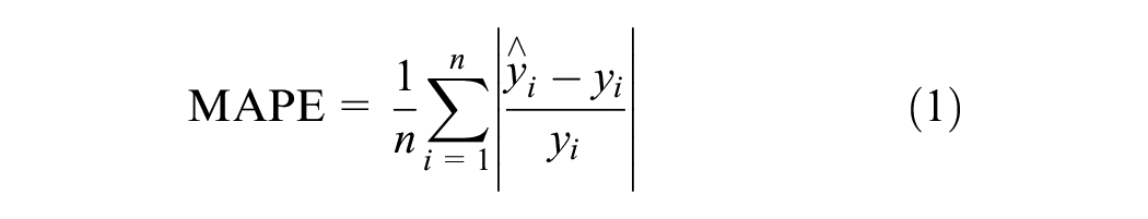
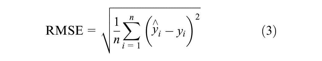
where

ŷ_i = predicted operation delay times for the ith incident,

y_i = actual operation delay times for the ith incident, and

n = the number of incidents.

Data Collection and Model Specification

The urban railway incident records were collected from an urban railway system in Hong Kong. The records were excluded from the modeling analysis if they had some missing information on any details. A total of 2,131 records with operation delays of at least 5 min between January 2012 and November 2018 were used for the analysis. We refer the interested readers to Chen et al. for the detailed description of incident datasets ( 15 ). A total of 12 explanatory variables are used for prediction modeling: day of the week, time of the day, season, weather, signal control system, affected line, operation direction, incident location, terminal/departure station, transfer station, affected area, and incident type. Table 1 introduces the explanatory variables and their distribution characteristics. As mentioned above, the AFT model assumes a linear relationship between the log of incident delays and various explanatory variables. To ensure prediction evaluation fairness, we conduct the log transform for operation delays (the dependent variable in the AFT model) and treat them as the dependent variable (e.g., prediction outcome) for all the selected models. Please note that log transformation also can reduce the variation of dependent variables and enhance the prediction performance to some extent, especially for skewed data ( 5 ). Figure 1 presents the distribution of disruption delays (log-transformed).

Table 1.

The Descriptive Statistics of Explanatory Variables (adapted from Chen et al.) ( 15 )

Category	% of observations
Day of week
Weekday	79.3%
Weekend	20.7%
Time of day
Non-peak	65.0%
Morning peak (07:00–09:00)	20.4%
Evening peak (17:00–19:00)	14.6%
Season
Spring	23.3%
Summer	27.8%
Fall	23.1%
Winter	25.8%
Weather
Sunny/cloudy	55.7%
Rainy	44.3%
Signal control system
Fixed block	87.9%
Moving block	12.1%
Line type
Line1	6.8%
Line2	23.2%
Line3	3.0%
Line4	0.4%
Other urban lines	66.6%
Operation direction
One-way direction	85.4%
Two-way direction	14.6%
Incident location
Ground	24.0%
Underground	50.7%
Elevated	25.3%
Terminal/departure station
No	69.9%
Yes	30.1%
Transfer station
No	54.0%
Yes	46.0%
Affected area
Single station	85.4%
Several stations	14.6%
Disruption type
PAD	13.5%
APG	2.6%
PSD	5.1%
Vehicle equipment failure	20.4%
Vehicle door failure	14.9%
Power equipment failure	4.8%
Power cable failure	1.0%
Track equipment failure	2.8%
Track crash without casualty	6.0%
Communication equipment failure	20.5%
Operation internal	6.8%
Operation external	1.6%

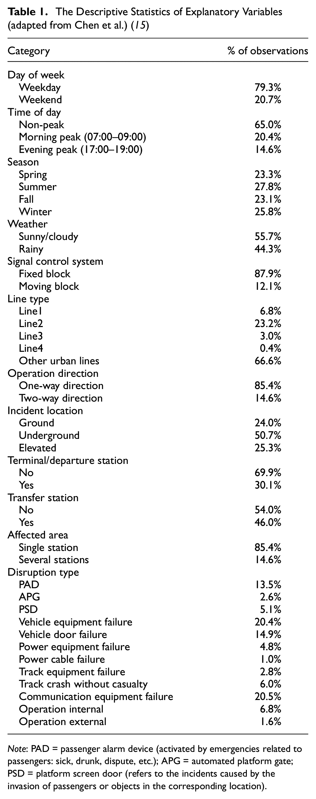
Note: PAD = passenger alarm device (activated by emergencies related to passengers: sick, drunk, dispute, etc.); APG = automated platform gate; PSD = platform screen door (refers to the incidents caused by the invasion of passengers or objects in the corresponding location).

Figure 1.

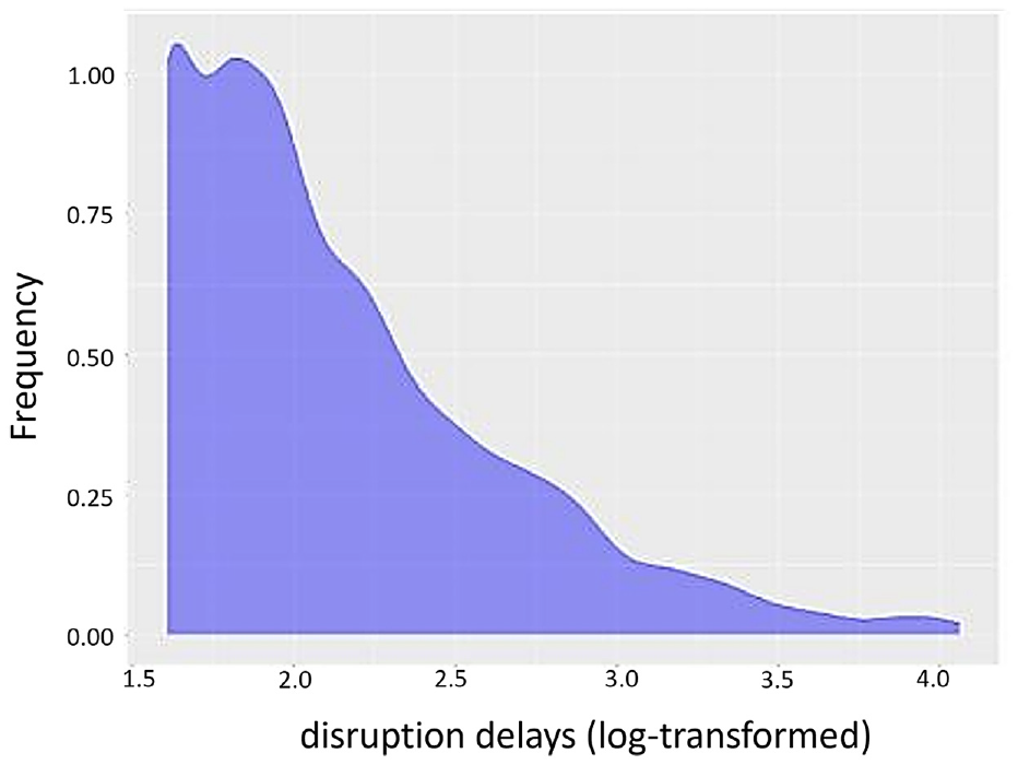
Distribution of disruption delays (log-transformed).

Model Results and Discussion

Model Parameters Optimization

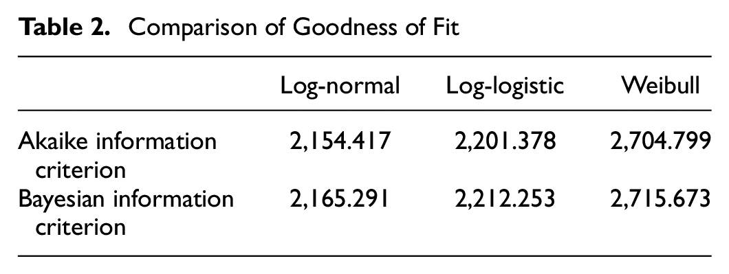
In this study, the dataset is randomly split into training data (70%) and test data (30%). In the process of model estimation, parameter optimization is a crucial step to improve the goodness of fit and prediction performance. For the AFT model, three distributions—Weibull, log-normal, and log-logistic—are tested. The best-fitted distribution is determined by the Akaike information criterion (AIC) and Bayesian information criterion (BIC). The smaller values of AIC and BIC represent better data fitting performance. As shown in Table 2, the log-normally distributed AFT model has the best performance. Therefore, the log-normal distribution is selected to fit the operation delays. The QR model is estimated at the 25^th, 50^th, 75^th, and 95^th percentiles. According to the modeling results, the QR model at the 25^th percentile outperforms the models at other quantiles. The distribution of operation delays also shows that the delays concentrate on short delays and, therefore, the 25^th QR model is used to predict the operation delays.

Table 2.

Comparison of Goodness of Fit

	Log-normal	Log-logistic	Weibull
Akaike information criterion	2,154.417	2,201.378	2,704.799
Bayesian information criterion	2,165.291	2,212.253	2,715.673

Bayesian optimization approach is used for parameter tuning in machine/ensemble learning models. The Bayesian optimization is packaged in Python, namely the Hyperopt package ( 33 ). The Hyperopt package has four objects: the objective function, search space, optimization algorithm, and the maximum number of evaluations ( 10 ). In this study, the target model function and its arguments are set as objective function and search space, respectively. The tree-structural Parzen estimator approach is selected as the optimization algorithm. The maximum number of evaluations is set as 100. In this study, parameter optimization for machine/ensemble learning models aims to select the optimal parameter with the lowest MAPE. Table 3 shows the parameters setting optimization in each model.

Table 3.

Model Parameter Setting and Optimization

Model	Parameter	Value set	Optimal parameters
KNN	K	[1,100]	39
SVR	Kernel function Penalty C	Linear, RBF, sigmoid [1,100]	Linear 34
RF	Maximum tree depth # of estimators	[1,12] [1,500]	4 350
GBDT	Maximum tree depth # of estimators Learning rate	[1,12] [1,500] [0.001,1]	2 100 0.08
Adaboost	Maximum tree depth # of estimators Learning rate	[1,12] [1,500] [0.001,1]	5 20 0.007
XGBoost	Maximum tree depth # of estimators Learning rate	[1,12] [1,500] [0.001,1]	4 70 0.037

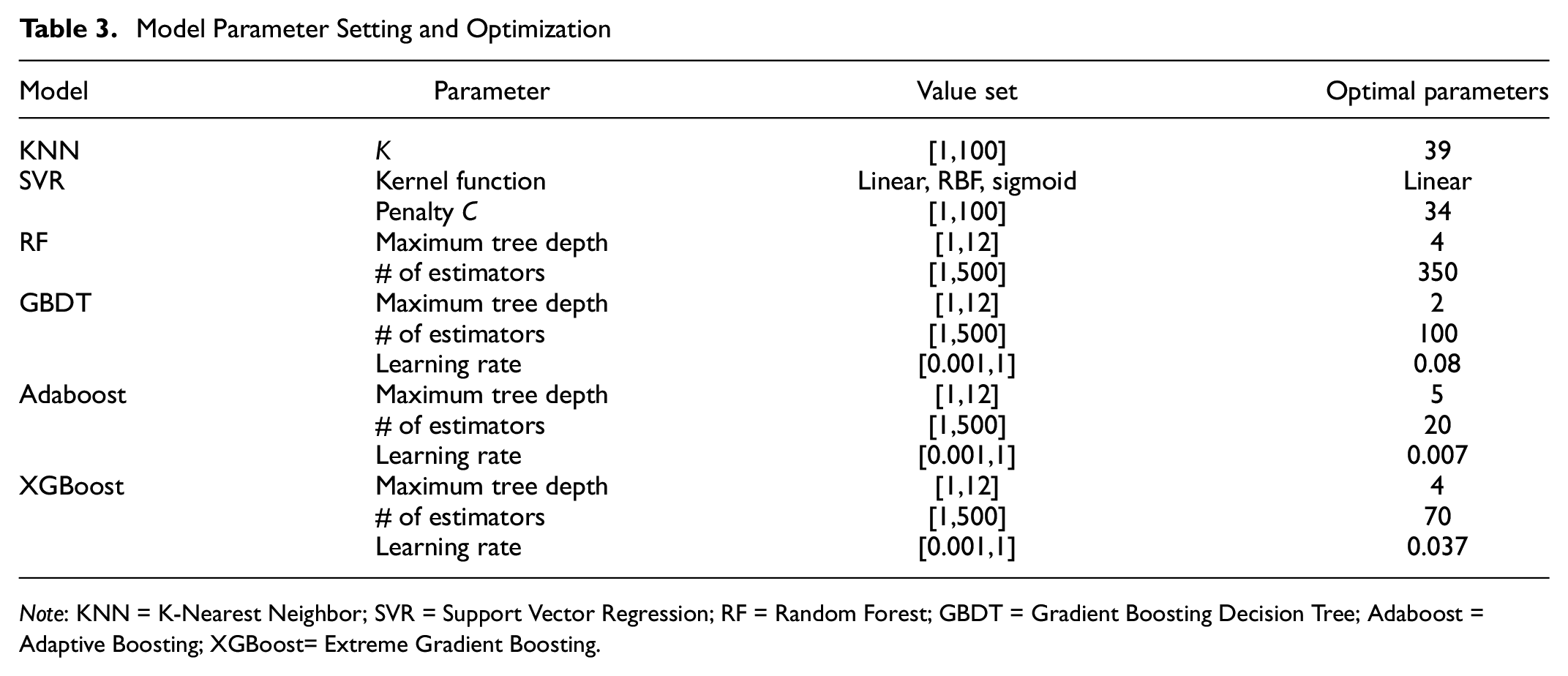
Note: KNN = K-Nearest Neighbor; SVR = Support Vector Regression; RF = Random Forest; GBDT = Gradient Boosting Decision Tree; Adaboost = Adaptive Boosting; XGBoost= Extreme Gradient Boosting.

Model Prediction Accuracy

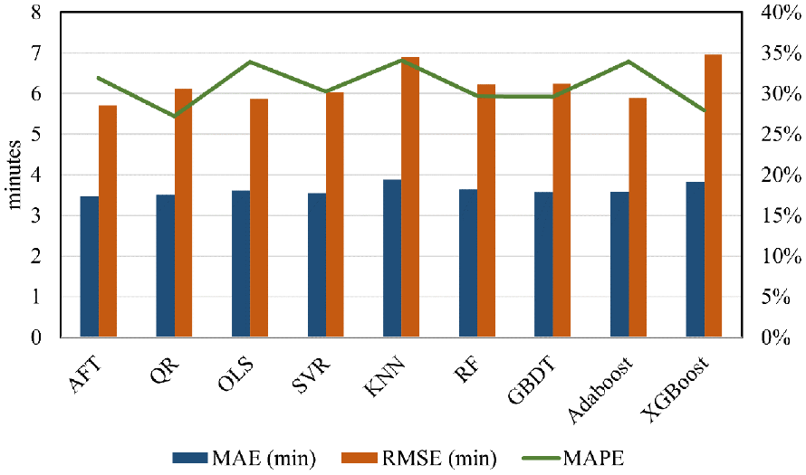
We adopt the 10 times leave-X (the length of testing data) out cross-validation method to obtain the average predicted results for performance evaluation. Figure 2 summarizes model prediction performance, including MAE, MAPE, and RMSE.

Figure 2.

Comparison of prediction accuracy.

Generally, the statistical models perform relatively better than machine/ensemble learning models in MAE and RMSE. For MAPE, the QR and XGBoost outperform other models, and the QR model exceeds the performance of XGBoost. The AFT model outperforms the other models in MAE and RMSE.

For the statistical models, the QR model provides the best prediction performance in MAPE while the OLS model performs worst among them. Given that the distribution of operation delays in this study is skewed, while the OLS model tends to capture the relationship between the mean value of operation delays and explanatory variables, this may lead to the issue of overestimation ( 6 ). The AFT model is established based on two strong assumptions of the random error term. The first is to assume that the error terms are uncorrelated with each other and the second is to assume that the error term is uncorrelated with explanatory variables ( 34 ). However, these two assumptions often fail because of the unobserved heterogeneity and, consequently, lead to the deviation of estimates ( 5 ). According to the results of the QR model, it has an error reduction of 4.69% compared with the AFT model. The reason could be that, instead of concentrating on exploring a single trend to summarize the disruption delay, QR focuses on multiple trends of delay at different quantiles to capture the disparity in trends caused by heterogeneity. Therefore, it is evident that the QR model can capture the unobserved heterogeneity, and thus has a better performance compared with those models without considering heterogeneity.

For traditional machine learning models, the SVR model has a more stable and accurate prediction performance than the KNN model in dealing with outliers. Outliers are the observations that significantly deviate from the other observations and usually have a negative impact on prediction accuracy ( 35 ). The predicted value of the KNN model is obtained by averaging the value of the K nearest neighbors around the target, which is highly affected by the possibly existing outliers. The SVR model constructs a hyperplane to minimize the distance to the targets and introduces relaxation factors to reduce the impact of outliers ( 36 ). In addition, the SVR model tends to perform well when using small samples.

As far as ensemble learning models are concerned, the XGBoost model gives a significantly lower value of MAPE, which implies the XGBoost model outperforms the other machine learning methods in predicting operation delays. This is because the XGBoost model applies the regularization item and greedy algorithm to improve the prediction ability ( 37 ). In addition, the XGBoost model also uses a second-order Taylor expansion of the loss function to enhance the generalization capacity. For the Adaboost model, larger weights are assigned to samples with larger prediction errors in the training process. Consequently, larger weights are easily assigned to outliers ( 20 ). Furthermore, the imbalance between different levels of categorical variables also makes the Adaboost model assign larger weights to samples with rare levels. Therefore, the MAPE value of the Adaboost model is significantly higher than other learning models, since it has a lower tolerance toward outliers. The GBDT model applies the gradient boosting method to improve the model. The sub-models of GBDT are trained sequentially, and each model is used to correct the error produced by the predecessors ( 11 ). The RF model is more tolerant to outliers, since it uses the random bootstrap sampling method. The chance of selecting outliers is much lower than in the other learning models ( 38 ). In addition, the final predicted result of the RF model is obtained by averaging the predicted result of each tree, which also improves the robustness.

The Effect of Influential Factors

In addition to operation delay prediction, we also explored the influential factors affecting operation delays. Statistical models generally are more interpretable, as they have explicit formulations about the relationship between explanatory variables and independent variables ( 39 ). We can interpret factors’ impact in statistical models based on the sign of coefficients and their significance levels. The machine/ensemble learning models focus on prediction accuracy rather than the causal relationship between explanatory variables and dependent variables ( 40 ). The opacity of these learning models makes it challenging to interpret what the model obtains in the prediction results ( 41 ). Since there is no specific rule to select the significant factors for machine/ensemble learning models, the relative importance of each variable is used for comparative analysis.

We select the five most influential or important factors in each model. For statistical models, we select the five most significant factors based on the standardized coefficients. For the tree-based model, the relative importance is calculated to compare the contribution of each factor. For the SVR model, we use the standardized weight to show the importance of each factor. The KNN model is not included, since it cannot output information related to importance.

Table 4 shows the five most influential factors in each model. Generally, the factors of the time of the day, signal control system, affected line, operation direction, incident location, affected area, and incident type are considered to significantly influence operation delays. For statistical models, the incident type, line type, and incident location all have a significant effect on urban railway operation delays. For machine/ensemble learning models, the incident type, line type, and affected area are the important influential factors.

Table 4.

Five Most Influential Factors of Each Model

Model	Factors
OLS	Incident type, affected line, operation direction, incident location, time of the day
AFT	Incident type, affected line, operation direction, incident location, signal control system
QR	Incident type, affected line, affected area, time of the day, incident location
SVR	Incident type, affected line, operation direction, signal control system, affected area
RF	Incident type, affected line, operation direction, affected area, signal control system
GBDT	Incident type, affected line, time of the day, incident location, affected area
Adaboost	Incident type, affected line, affected area, incident location, time of the day
XGBoost	Incident type, affected line, affected area, incident location, time of the day

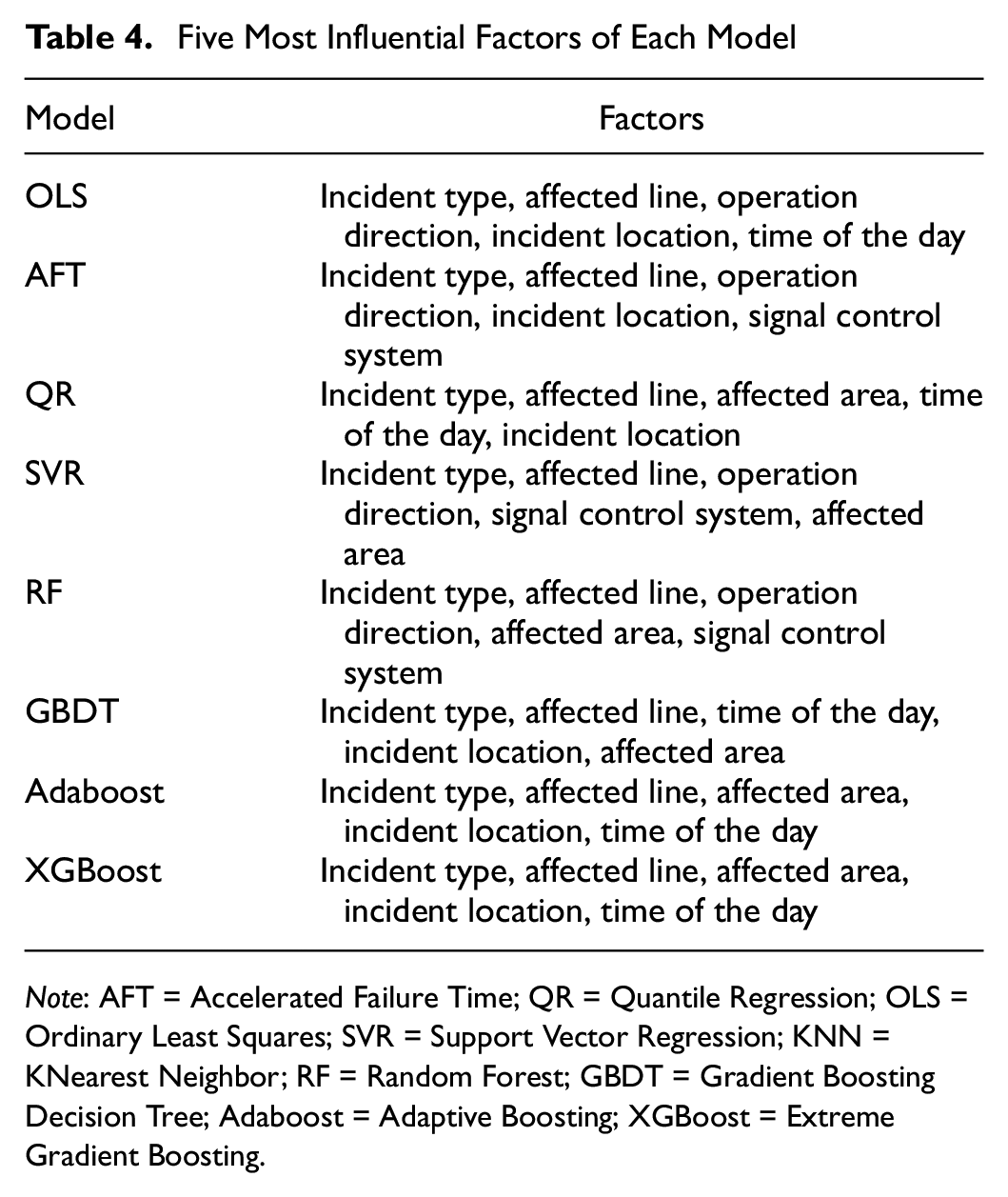
Note: AFT = Accelerated Failure Time; QR = Quantile Regression; OLS = Ordinary Least Squares; SVR = Support Vector Regression; KNN = KNearest Neighbor; RF = Random Forest; GBDT = Gradient Boosting Decision Tree; Adaboost = Adaptive Boosting; XGBoost = Extreme Gradient Boosting.

Among the selected influential factors, the incident type and affected line consistently rank the first and second in all models. The incident type is considered to seriously affect operation delays in many studies ( 3 , 5 , 10 ). The main reason could be that a couple of adverse causes, such as power cable failure and external operation failure, may have a great impact on operation delays in all incident types. Because of the length and complexity of the power cables, it is difficult to determine the fault location quickly and accurately ( 42 ). External operation failure includes bad weather and crashes with the casualty. The occurrence of adverse weather (storms, floods, etc.) directly leads to the disruption of the urban railway system. For the crashes with casualties, it is reasonable for the staff to spend more time coping with them ( 3 ).

The affected line type also affects operation delay since the type of vehicle, the staff working ability, and the geographical environment differ on different routes. In addition, many factors increase the complexity of the incident and thus prolong operation delays to some extent. These factors include operation direction (e.g., one-way or two-way), incident location (ground, underground, or elevated), and affected area (single station or several stations). When a failure occurs, a more complex incident usually leads to longer operation delays for inspecting and fixing. The signal control system can be divided into the fixed-block system and the moving-block system. Once a failure occurs in the signal control system, the repair of the moving-block system is more time-consuming than the fixed-block system. In addition, an incident occurring during the peak period is likely to have longer delays.

In summary, from the perspective of prediction accuracy, the statistical model QR, traditional machine learning model SVR, and ensemble learning model XGBoost present a significantly low value of MAPE. From the perspective of influential factors, the estimated results of QR and XGBoost present a similar empirical finding.

Discussion and Conclusion

Accurate delay prediction is important for the effective management of urban railway incidents. This paper conducts a methodology review for predicting delays using a large-scale incident logs dataset in an urban railway system. Three statistical methods (OLS, AFT, QR) and six machine/ensemble learning methods (KNN, SVR, RF, GBDT, Adaboost, and XGBoost) are examined. The comparative study shows that statistical models perform relatively better than machine/ensemble learning models in predicting train delays under incidents. The QR and XGBoost model performed best (in MAPE) in statistical and machine/ensemble learning models, respectively. Furthermore, the QR model outperforms XGBoost in terms of MAPE (0.68%), MAE (8.33%), and RMSE (13.73%). For machine/ensemble learning methods, KNN and Adaboost models have a significantly higher prediction error, indicating that models sensitive to outliers are likely to have a significantly lower prediction accuracy. The factors of the incident type and affected line type present the most significant effects on incident delay prediction in selected models.

Generally, the tested models show different performance for incident delay prediction, as far as the prediction accuracy and influential factor interpretability are concerned. The results provide insights for transit authorities/practitioners in choosing suitable models to serve their targets. For example, an agency can choose suitable models to predict approximate delays caused by unplanned disruptions. Through such prediction, the agency can inform affected travelers to adjust their travel plans (e.g., information provision) and/or inform operators to adjust service schedules (e.g., timetable), thus reducing risk of secondary delays and avoiding large crowds on platforms/systems during disruptions. In addition, according to the statistical relationship (e.g., the sign and significance level) between delay and explanatory variables, the agency can improve transit performance and service through infrastructure upgrade/investments and alternative service deployments. For example, given that an incident type shows the highest correlation with long disruption delays in the urban railway system, the practitioners can upgrade corresponding equipment (e.g., vehicle, communication, and power) to reduce the likelihood of disruption occurrence. Also, the agency should pay more attention to specific operational lines/stations through real-time monitors/observations, assigning more staff, as well as deploying shuttle buses, for a timely response to manage disruptions.

The main limitation of this research is that we only analyzed the incident dataset collected from one urban railway system, in Hong Kong. Therefore, the research findings are likely to be constrained to the specific context of that railway system and may not be confidently generalized to other cases. However, we do think the empirical findings from our case study would enrich the literature in a Hong Kong context. Future work can focus on collecting more urban railway incident records from different urban railway systems and/or a meta-review and cross-analysis of evidence from other cities to draw generic conclusions.

Footnotes

Acknowledgements

The authors would like to acknowledge the Urban Railway Company for providing the data. The authors thank the handling editor and reviewers for their constructive comments to improve the quality of this paper.

Author Contributions

The authors confirm contribution to the paper as follows: study conception and design: X. Chen, Z. Ma; data collection: X. Chen, W. Sun; analysis and interpretation of results: X. Chen, Z. Ma, W. Sun; draft manuscript preparation: W. Sun, X. Chen, Z. Ma. All authors reviewed the results and approved the final version of the manuscript.

Declaration of Conflicting Interests

The author(s) declared no potential conflicts of interest with respect to the research, authorship, and/or publication of this article.

Funding

The author(s) disclosed receipt of the following financial support for the research, authorship, and/or publication of this article: The work was funded by Swedish Strategic Research Funding in Transportation (TRENoP).

ORCID iD

Zhenliang Ma

References

Chung

Development of an Accident Duration Prediction Model on the Korean Freeway Systems. Accident Analysis & Prevention, Vol. 42, No. 1, 2010, pp. 282–289.

Garib

Radwan

Al-Deek

Estimating Magnitude and Duration of Incident Delays. Journal of Transportation Engineering, Vol. 123, No. 6, 1997, pp. 459–466.

Weng

Zheng

Yan

Meng

Development of a Subway Operation Incident Delay Model Using Accelerated Failure Time Approaches. Accident Analysis & Prevention, Vol. 73, 2014, pp. 12–19.

Weng

Feng

Xiong

Maximum Likelihood Regression Tree with Two-Variable Splitting Scheme for Subway Incident Delay. Transportmetrica A: Transport Science, Vol. 15, No. 2, 2019, pp. 1061–1080.

Tang

Zheng

Han

Yin

Zhang

Zou

Huang

Statistical and Machine-Learning Methods for Clearance Time Prediction of Road Incidents: A Methodology Review. Analytic Methods in Accident Research, Vol. 27, 2020, p. 100123.

Khattak

A. J.

Liu

Wali

Modeling Traffic Incident Duration Using Quantile Regression. Transportation Research Record: Journal of the Transportation Research Board, 2016. 2554: 139–148.

Yap

Cats

Predicting Disruptions and Their Passenger Delay Impacts for Public Transport Stops. Transportation, Vol. 48, No. 4, 2021, pp. 1703–1731.

Wen

Chen

S. Y.

Xiong

Q. Y.

Han

R. B.

Chen

S. Y.

Traffic Incident Duration Prediction Based on K-Nearest Neighbor. Applied Mechanics and Materials, Vol. 253, 2013, pp. 1675–1681.

W.-w.

Chen

S.-y.

Zheng

C.-j.

Traffic Incident Duration Prediction Based on Support Vector Regression. Proc., ICCTP 2011: Towards Sustainable Transportation Systems, Nanjing, China, 2011, pp. 2412–2421.

10.

Tang

Zheng

Han

Liu

Cai

Traffic Incident Clearance Time Prediction and Influencing Factor Analysis Using Extreme Gradient Boosting Model. Journal of Advanced Transportation, Vol. 2020, 2020, p. 6401082.

11.

Yang

Chen

Ensemble Learning for Short-Term Traffic Prediction Based on Gradient Boosting Machine. Journal of Sensors, Vol. 2017, 2017, p. 7074143.

12.

Kockelman

K. M.

How Does Machine Learning Compare to Conventional Econometrics for Transport Data Sets? A Test of ML Versus MLE. Growth and Change, Vol. 53, No. 1, 2022, pp. 342–376.

13.

Zhang

Yan

Wang

A Comparative Study of Prediction Models on the Duration of Traffic Incidents. Proc., International Conference on Transportation and Development, American Society of Civil Engineers, Reston, VA, 2020.

14.

Liu

Wang

Predicting Subway Incident Delays Using Text Analysis Based Accelerated Failure Time Model. Journal of Transportation Safety & Security, Vol. 13, No. 3, 2021, pp. 340–356.

15.

Chen

Unplanned Disruption Analysis and Impact Modeling in Urban Railway Systems. Transportation Research Record: Journal of the Transportation Research Board, Vol. 2676, No. 10, 2022, pp. 16–27.

16.

Tiong

K. Y.

Palmqvist

C.-W.

A Review of Data-Driven Approaches to Predict Train Delays. Transportation Research Part C: Emerging Technologies, Vol. 148, 2023, p. 104027.

17.

Liu

Koutsopoulos

H. N.

, Modeling the Duration of the Impact of Unplanned Disruptions on Passenger Trips Using Smartcard Data in Urban Rail Systems. Urban Rail Transit, Vol. 9, No. 3, pp. 266–279.

18.

Ding

Luan

Wang

Prioritizing Influential Factors for Freeway Incident Clearance Time Prediction Using the Gradient Boosting Decision Trees Method. IEEE Transactions on Intelligent Transportation Systems, Vol. 18, No. 9, 2017, pp. 2303–2310.

19.

Akçay

M. T.

Akgundogdu

Tiryaki

Prediction of Travel Time for Railway Traffic Management by Using the AdaBoost Algorithm. Balıkesir Üniversitesi Fen Bilimleri Enstitüsü Dergisi, Vol. 24, No. 1, 2022, pp. 300–312.

20.

Jumaah

H. J.

Ameen

M. H.

Kalantar

Rizeei

H. M.

Jumaah

S. J.

Air Quality Index Prediction Using IDW Geostatistical Technique and OLS-Based GIS Technique in Kuala Lumpur, Malaysia. Geomatics, Natural Hazards and Risk, Vol. 10, No. 1, 2019, pp. 2185–2199.

21.

Hensher

D. A.

Mannering

F. L.

Hazard-Based Duration Models and Their Application to Transportation Analysis. Working Paper ITS-WP-93-1. Institute of Transport Studies, Graduate School of Business, The University of Sydney, NSW, 1993.

22.

Koenker

Bassett

Jr.

Regression Quantiles. Econometrica: Journal of the Econometric Society, Vol. 46, No. 1, 1978, pp. 33–50.

23.

Nowotarski

Weron

Computing Electricity Spot Price Prediction Intervals Using Quantile Regression and Forecast Averaging. Computational Statistics, Vol. 30, No. 3, 2015, pp. 791–803.

24.

Cortes

Vapnik

Support-Vector Networks. Machine Learning, Vol. 20, No. 3, 1995, pp. 273–297.

25.

Application on Traffic Flow Prediction of Machine Learning in Intelligent Transportation. Neural Computing and Applications, Vol. 33, No. 2, 2021, pp. 613–624.

26.

Breiman

Random Forests. Machine Learning, Vol. 45, No. 1, 2001, pp. 5–32.

27.

Breiman

Bagging Predictors. Machine Learning, Vol. 24, No. 2, 1996, pp. 123–140.

28.

Schapire

R. E.

The Strength of Weak Learnability. Machine Learning, Vol. 5, No. 2, 1990, pp. 197–227.

29.

Freund

Schapire

R. E.

A Decision-Theoretic Generalization of On-Line Learning and an Application to Boosting. Journal of Computer and System Sciences, Vol. 55, No. 1, 1997, pp. 119–139.

30.

Freund

Schapire

R. E.

Adaptive Game Playing Using Multiplicative Weights. Games and Economic Behavior, Vol. 29, No. 1–2, 1999, pp. 79–103.

31.

Chen

Guestrin

Xgboost: A Scalable Tree Boosting System. Proc., 22nd ACM SIGKDD International Conference on Knowledge Discovery and Data Mining, San Francisco, CA, Association for Computing Machinery, New York, NY, 2016.

32.

Zhao

Deng

Prediction in Traffic Accident Duration Based on Heterogeneous Ensemble Learning. Applied Artificial Intelligence, Vol. 36, No. 1, 2022, p. 2018643.

33.

Yang

Fang

Zheng

Zhou

Peng

An expressway traffic incident detection method based on convolutional neural network and extreme gradient boosting. 2020. https://www.preprints.org/manuscript/202004.0248/v1.

34.

Hensher

D. A.

Mannering

F. L.

Hazard-Based Duration Models and Their Application to Transport Analysis. Transport Reviews, Vol. 14, No. 1, 1994, pp. 63–82.

35.

Lin

Brown

D. E.

An Outlier-Based Data Association Method for Linking Criminal Incidents. Decision Support Systems, Vol. 41, No. 3, 2006, pp. 604–615.

36.

Wang

Yao

Wang

A Comparison of the Performance of ANN and SVM for the Prediction of Traffic Accident Duration. Neural Network World, Vol. 26, No. 3, 2016, p. 271.

37.

Feng

Wang

Yin

An XGBoost-Based Casualty Prediction Method for Terrorist Attacks. Complex & Intelligent Systems, Vol. 6, No. 3, 2020, pp. 721–740.

38.

Iranitalab

Khattak

Comparison of Four Statistical and Machine Learning Methods for Crash Severity Prediction. Accident Analysis & Prevention, Vol. 108, 2017, pp. 27–36.

39.

Glymour

Madigan

Pregibon

Smyth

Statistical Inference and Data Mining. Communications of the ACM, Vol. 39, No. 11, 1996, pp. 35–41.

40.

Nasteski

An Overview of the Supervised Machine Learning Methods. Horizons B, Vol. 4, 2017, pp. 51–62.

41.

Price

Nicholson

Rai

A. K.

Clearing Opacity Through Machine Learning. Iowa Law Review, Vol. 106, 2020, pp. 775–812.

42.

Weng

Zheng

Yan

Development of a Maximum Likelihood Regression Tree-Based Model for Predicting Subway Incident Delay. Transportation Research Part C: Emerging Technologies, Vol. 57, 2015, pp. 30–41.

Incident Delay Prediction in Urban Railway Systems: Methodology Review and Exploratory Comparative Analysis

Abstract

Keywords

Methodology

Statistical Models

Ordinary Least Squares (OLS)

Accelerated Failure Time (AFT)

Quantile Regression (QR)

Traditional Machine Learning Models

Support Vector Machine (SVM)

Support Vector Regression (SVR)

K-Nearest Neighbor (KNN)

Ensemble Learning Models

Random Forest (RF)

Gradient Boosting Decision Tree (GBDT)

Adaptive Boosting (Adaboost)

Extreme Gradient Boosting (XGBoost)

Model Evaluation

Data Collection and Model Specification

Model Results and Discussion

Model Parameters Optimization

Model Prediction Accuracy

The Effect of Influential Factors

Discussion and Conclusion

Footnotes

Acknowledgements

Author Contributions

Declaration of Conflicting Interests

Funding

ORCID iD

References