Sage Journals: Discover world-class research

Abstract

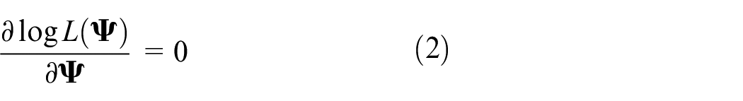
Railroad ballast is typically comprised of only large granular particles. However, the degradation of fresh ballast and the arrival of foreign fines result in ballast fouling. Compared with fresh ballast, fouled ballast exhibits reduced resilience and compromised drainage capabilities. To optimize track performance, maintenance activities for the ballast are frequently scheduled based on the fouling severity. An accurate assessment of ballast fouling conditions can enhance maintenance efficiency and reduce costs. Over the years, while many ballast fouling evaluation methods have been developed, their widespread adoption has been hindered by system costs and implementation challenges. This study aims to address this by developing an affordable and easily implemented approach to estimating ballast fouling conditions using the Gaussian Mixture Model (GMM). Initially, images of fouled ballast are characterized by fitting the distributions of each RGB (Red, Green, Blue) channel. Subsequently, two mathematical methods, expectation-maximization and point estimation, are employed to solve the GMM parameters. These derived GMM parameters are then used to backcalculate the sample parameters, facilitating the estimation of ballast fouling conditions. The results of this study reveal a close alignment between the ballast fouling conditions backcalculated with the GMM and those quantified through laboratory sieving analysis. This study thus presents a promising path forward, using images captured from cost-effective cameras to estimate ballast fouling conditions with minimal computational expense.

Keywords

rail railroad infrastructure design and maintenance ballast fouled inspection

The ballasted track is the dominant track structure for freight railroads. It relies on coarse-graded granular material ( 1 ). Typically crushed from igneous rocks such as granite or basalt, fresh ballast should conform to open-graded gradation requirements ( 2 , 3 ). It performs several essential functions, such as supporting the track, transferring train loads, providing drainage, and facilitating maintenance activities ( 2 ).

Despite ballast being engineered to resist wear and tear, train loads can lead to the breakdown of angular ballast particles ( 4 ). The resultant fines, combined with airborne and subgrade materials, contribute to the fouling materials ( 3 , 5 ). These fouling materials, even small enough to pass a No. 200 sieve (75 µm), can infiltrate and fill the voids within ballast particles. This fouling impairs the ballast drainage capability, leading to moisture retention, vegetation growth, and a subsequent decrease in drainage ability ( 2 ). The excessive moisture can also reduce ballast shear strength, increase permanent settlement rates ( 6 – 9 ), and increase the risk of mud pumping ( 10 ). Such conditions can cause increased rail bending stress at the mud spots ( 2 ). To mitigate potential risks to track safety, regular maintenance activities are essential for fouled ballast. An accurate assessment of ballast fouling conditions is important for efficient track maintenance ( 11 ). Several indices have been proposed to evaluate ballast fouling, including Fouling Index (FI), Volume Contaminant Index (VCI), and Percent Degraded Segments (PDS) ( 5 , 8 , 12 , 13 ).

Traditional methods for detecting ballast fouling conditions include sieve analysis for determining FI and Non-Destructive Testing (NDT) methods such as surface wave analysis, SmartRock trajectory, and Ground Penetration Radar ( 14 – 22 ). Modern computer vision technologies offer alternative solutions through machine learning ( 11 , 13 ), while hyperspectral imaging techniques have been used to characterize fouled ballast ( 23 ). However, these methods can be challenging to operate and computationally intensive. Recent work has identified a linear relationship between FI and the variance of the fouled ballast image color intensity, though it lacks a fundamental explanation ( 24 ).

The GMM, the weighted summation of several normal distributions, offers more flexibility in fitting unknown distributions ( 25 ). Especially useful when dealing with multi-component distributions, GMM has been employed to characterize soil types and properties in recent years ( 26 – 31 ).

This study uses GMM to characterize the color intensity of fouled ballast images. The linear relationship between sample variance and FI ( 24 ) is verified through GMM backcalculation. Noting that fouled ballast comprises large ballast particles, clustered fines, and voids, these three components of the fouled ballast RGB (Red, Green, Blue) distributions are decomposed using GMM. The GMM fitting parameters (component means, variances, and mixing portions) are estimated by two methods: expectation-maximization and point estimation. In this study, two assumptions are made to optimize fitting results, and two hypotheses are raised for further study.

Fouled Ballast Image

Earlier research collected and analyzed images of fouled ballast samples specifically designed to represent varying FI values, as depicted in Figure 1 ( 24 ). This ballast, composed of basalt, has undergone degradation after enduring 600 million gross tons (MGT) of train loading. It is gathered from the Rainy Section test track at the Transportation Technology Center. The majority of fouling materials originate from the degradation of the basalt ballast, with a minor proportion coming from the subgrade soil.

Figure 1.

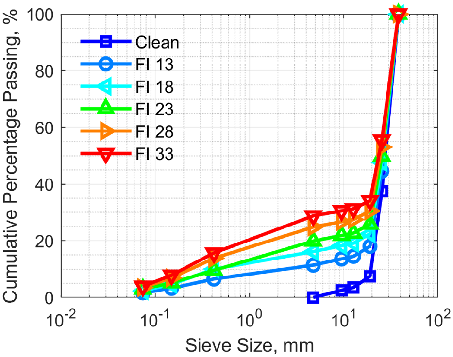
Gradation curves for fouled ballast.

Images of the fouled ballast are captured through transparent acrylic walls under controlled illumination conditions. Each FI value is associated with six images, each encompassing three color channels: Red, Green, and Blue. Each color channel possesses a relative frequency distribution, denoted as $f_{ijk}$ , which is detailed in Table 1. The sample means and variances can be derived from these relative frequency distributions.

Table 1.

Input Relative Frequency Distributions in This Study

FI, i		Picture sequence, j		Color channel, k		Relative frequency distribution
0	×	1	×	Red	→	$f_{ijk}$
13		2		Red
18		3		Green
23		4		Green
28		5		Blue
33		6		Blue

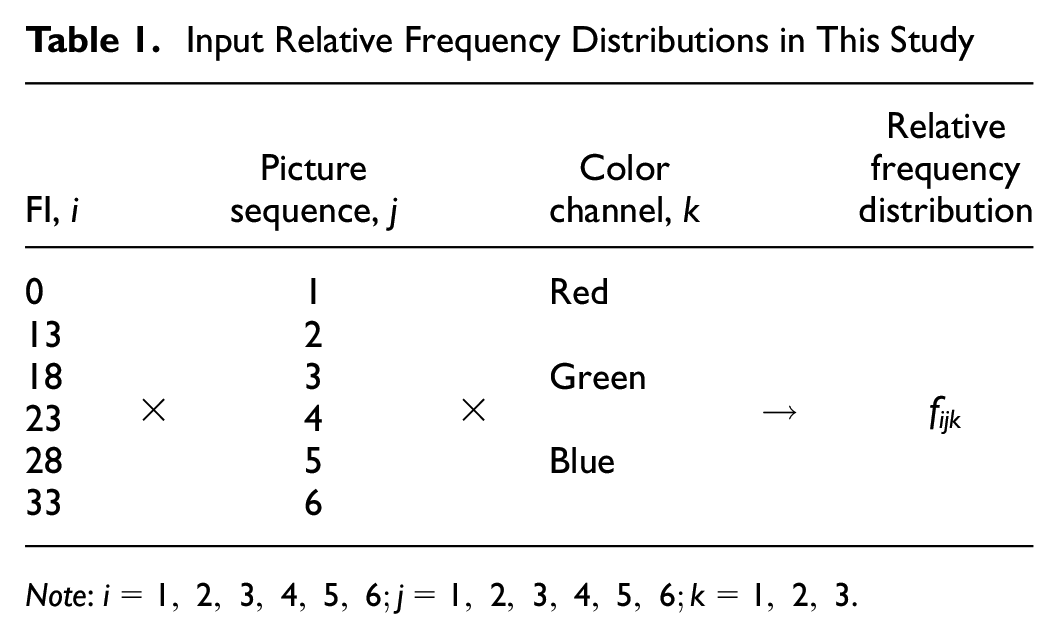
Note: $i = 1, 2, 3, 4, 5, 6; j = 1, 2, 3, 4, 5, 6; k = 1, 2, 3$ .

Figure 2 depicts the RGB color density distributions for a fouled ballast sample with an FI value of 18. The relative frequency plot is clearly asymmetrical for each channel, suggesting that the normal distribution model would not be an appropriate fit for these distributions. Knowing that a small value of one color channel corresponds to a dark color, the difference between the voids and the ballast should be reflected on the relative frequency plot. Similarly, the fouled ballast should be classified into large ballast particles and fines. Objectively, one distribution curve can be separated into three ranges through a trial-and-error process. Each distribution can be manually segmented into three ranges: the left tail, the left elbow, and the remaining portion. The three corresponding ranges for one distribution are shown below in the respective channel color, as presented in Figure 2. Regardless of the color channel, each range essentially highlights the same region across all three channels. Range 1 corresponds to the voids within the fouled ballast, while Range 3 symbolizes the surfaces of large ballast particles and clustered fines. Range 2 represents the edges of large particles or the clustered fines.

Figure 2.

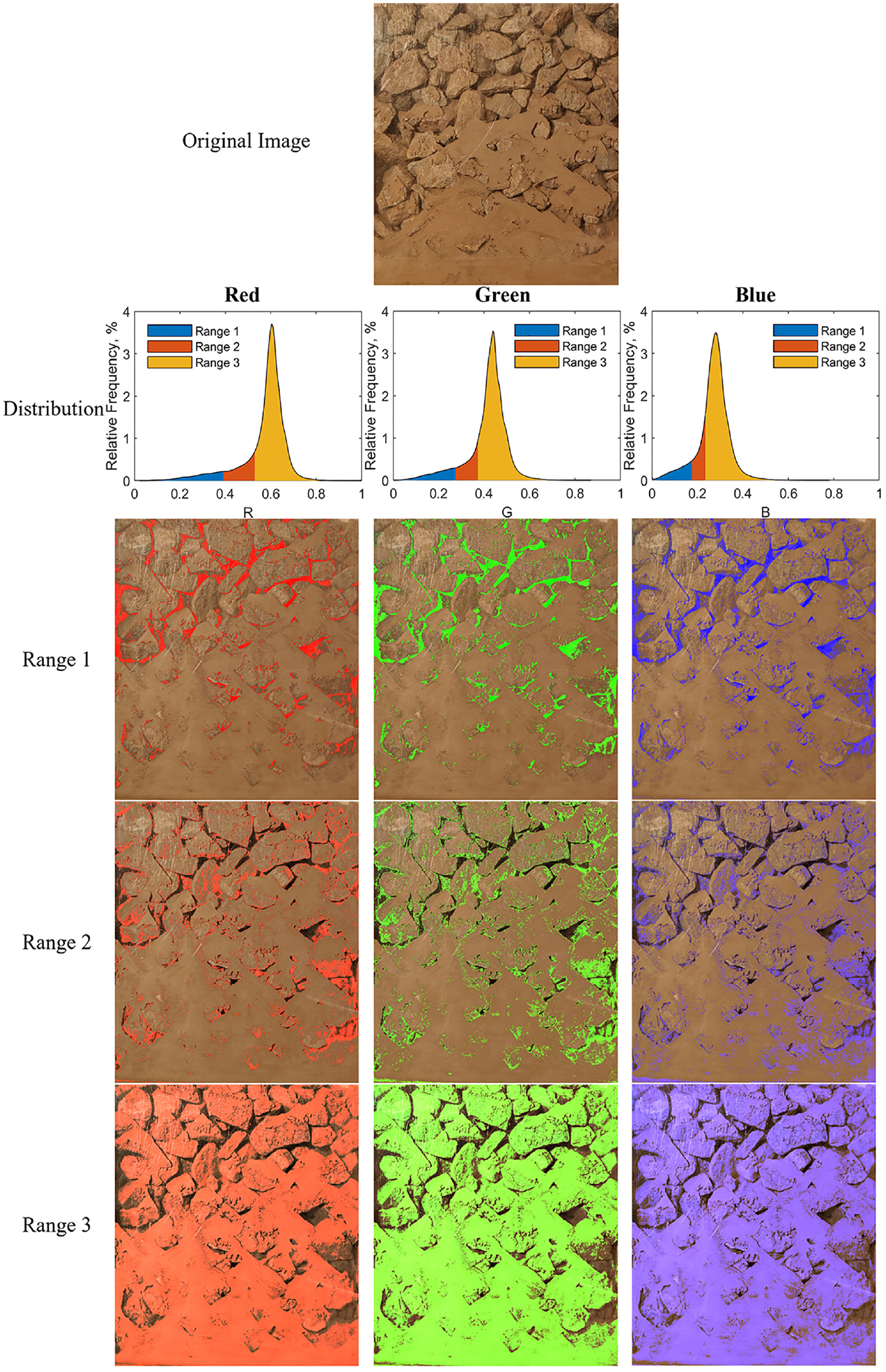
An example of fouled ballast (FI 18) image decomposition.

Given that fouled ballast consists of ballast particles, fines, and voids, each individual color channel illustrated in Figure 2 manifests this reality in the form of color channel intensity. Therefore, it is logical and reasonable to assume that a fouled ballast color intensity distribution comprises three distinct components. The relative frequency distributions in Figure 2 are not symmetric, which cannot be fitted well by a normal distribution, which only has two fitting parameters. Instead of assuming that the color intensity of one channel follows a normal distribution, each component of the fouled ballast image could follow a normal distribution.

Gaussian Mixture Model

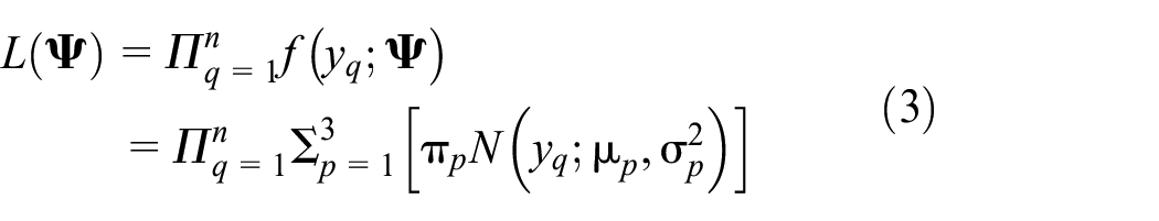
A GMM can be described as a multivariate distribution synthesized by a finite number of Gaussian or normal distributions. Each Gaussian distribution is treated as an independent normal distribution, complete with its own mean and covariance. These normal distributions are combined proportionally, each representing their respective fractions of the GMM population ( 25 ). Given that the image intensity data are processed for each color channel, the normal distribution employed in this study is one-dimensional, reducing covariance to variance.

The following equation describes the GMM in this study, which is a probability density function:

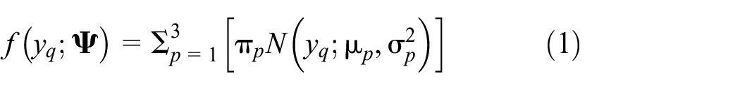
\begin{matrix} f (y_{q}; Ψ) = Σ_{p = 1}^{3} [π_{p} N (y_{q}; μ_{p}, σ_{p}^{2})] \end{matrix}

(1)

where the vector $y = {(y_{1}, y_{2}, \dots, y_{n})}^{T}$ is the observed color intensity data in one dimension, and the vector $Ψ = {(π_{1}, π_{2}, μ^{T}, {σ^{2}}^{T})}^{T}$ is the parameter vector that needs to be determined. The vector $π = {(π_{1}, π_{2}, π_{3})}^{T}$ denotes the mixing portion. Each distribution component has its own mean $μ_{p}$ and variance $σ_{p}^{2}$ .

Because the summation of mixing portions is 1, there are only two independent mixing portion parameters, making the number of elements in the parameter vector $Ψ$ eight instead of nine. The most commonly used approach to the estimation of $Ψ$ , $\hat{Ψ}$ , is the maximum likelihood. The maximum likelihood estimator, $\hat{Ψ}$ , is the global maximizer of the likelihood. Elements of $\hat{Ψ}$ are the roots which satisfy the following equation ( 25 ):

\frac{\partial \log L (Ψ)}{\partial Ψ} = 0

(2)

where the likelihood function for $Ψ$ :

\begin{matrix} L (Ψ) & = π_{q = 1}^{n} f (y_{q}; Ψ) \\ \begin{matrix} = π_{q = 1}^{n} Σ_{p = 1}^{3} [π_{p} N (y_{q}; μ_{p}, σ_{p}^{2})] \end{matrix} \end{matrix}

(3)

The maximum likelihood estimator, $\hat{Ψ}$ , satisfies:

\begin{matrix} {\hat{π}}_{p} = \frac{Σ_{q = 1}^{n} τ_{p} (y_{q}; \hat{Ψ})}{n} (p = 1, 2, 3) \end{matrix}

(4)

and

\begin{matrix} Σ_{p = 1}^{3} Σ_{q = 1}^{n} τ_{p} (y_{q}; \hat{Ψ}) \frac{\partial \log N (y_{q}; μ_{p}, {\hat{σ^{2}}}_{p})}{\partial μ_{p}} = 0 \end{matrix}

(5)

and

\begin{matrix} Σ_{p = 1}^{3} Σ_{q = 1}^{n} τ_{p} (y_{q}; \hat{Ψ}) \frac{\partial \log N (y_{q}; {\hat{μ}}_{p}, σ_{p}^{2})}{\partial σ_{p}^{2}} = 0 \end{matrix}

(6)

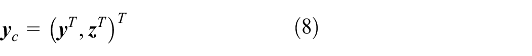
A 3-D vector of zero-one indicator variables, $z_{q}$ , is defined to indicate whether the qth observed value, $y_{q}$ , belongs to the pth component of the mixture. All the $z_{q}$ vectors form a labeling vector $z = {(z_{1}^{T}, \dots, z_{n}^{T})}^{T}$ , where $z_{pq} = {(z_{q})}_{p}$ . The $z_{pq}$ can be expressed by the posterior probability, $τ_{p} (y_{q}; Ψ)$ , that the qth observed value belongs to the pth component of the mixture ( 32 ):

\begin{matrix} z_{pq} = τ_{p} (y_{q}; \hat{Ψ}) = \frac{{\hat{π}}_{p} N (y_{q}; μ_{p}, σ_{p}^{2})}{f (y_{q}; \hat{Ψ})} \end{matrix}

(7)

Associated with the labeling vector $z$ , the observed data vector $y$ , forms the complete-data vector ( 25 ):

\begin{matrix} y_{c} = {(y^{T}, z^{T})}^{T} \end{matrix}

(8)

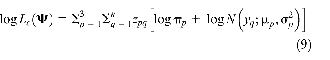
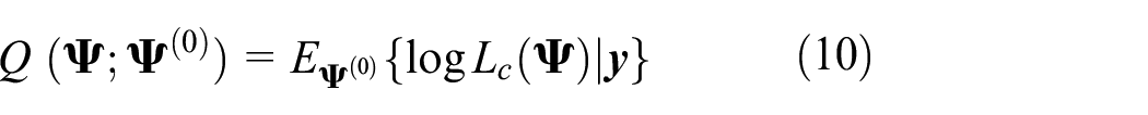
The complete-data log-likelihood for $Ψ$ , $\log L_{c} (Ψ)$ , is given by ( 25 ):

\begin{matrix} \log L_{c} (Ψ) = Σ_{p = 1}^{3} Σ_{q = 1}^{n} z_{pq} [\log π_{p} + \log N (y_{q}; μ_{p}, σ_{p}^{2})] \end{matrix}

(9)

Expectation-Maximization

The expectation-maximization (EM) algorithm involves two steps, E- (for expectation) and M- (for maximization), to iteratively solve for $\hat{Ψ}$ ( 25 ).

E-Step

The initial guess of $Ψ$ , $Ψ^{(0)}$ , yields the conditional expectation of $\log L_{c} (Ψ)$ given $y$ :

Q (Ψ; Ψ^{(0)}) = E_{Ψ^{(0)}} {\log L_{c} (Ψ) | y}

(10)

According to the property of $z_{pq}$ in Equation (7), the current conditional expectation of $Z_{pq}$ , where $Z_{pq}$ is the corresponding random variable to $z_{pq}$ , given the observed data $y$ , as follows:

\begin{matrix} E_{Ψ^{(0)}} {Z_{pq} | y} = τ_{p} (y_{q}; Ψ^{(0)}) \end{matrix}

(11)

Noticing that is the linear relationship between $\log L_{c} (Ψ)$ and $z_{pq}$ , the first conditional expectation of $\log L_{c} (Ψ)$ given $y$ is:

\begin{matrix} Q (Ψ; Ψ^{(0)}) = Σ_{p = 1}^{3} Σ_{q = 1}^{n} τ_{p} (y_{q}; Ψ^{(0)}) [\log π_{p} + \log N (y_{q}; μ_{p}, σ_{p}^{2})] \end{matrix}

(12)

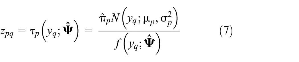
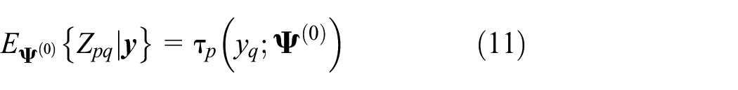
On the (r+1)th iteration, the E-step calculates $Q (Ψ; Ψ^{(r)})$ , where $Ψ^{(r)}$ is the value $Ψ$ of after the rth EM iteration:

\begin{matrix} Q (Ψ; Ψ^{(r)}) = Σ_{p = 1}^{3} Σ_{q = 1}^{n} τ_{p} (y_{q}; Ψ^{(r)}) [\log π_{p} + \log N (y_{q}; μ_{p}, σ_{p}^{2})] \end{matrix}

(13)

as the current conditional expectation $z_{pq}^{(r)} = τ_{p} (y_{q}; Ψ^{(r)})$ .

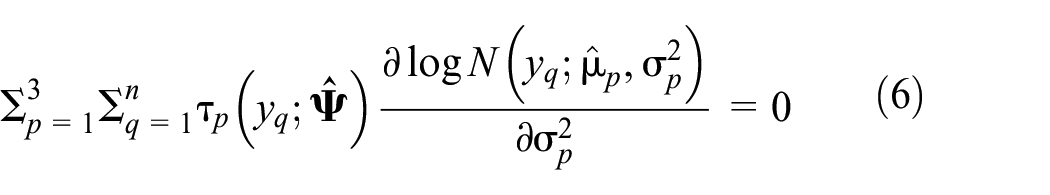
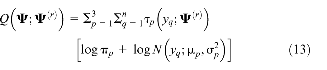
M-Step

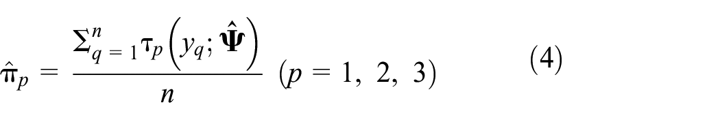
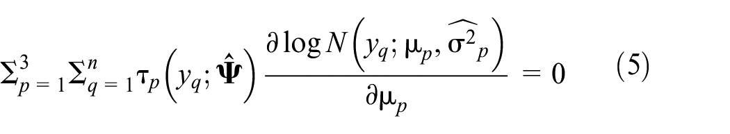
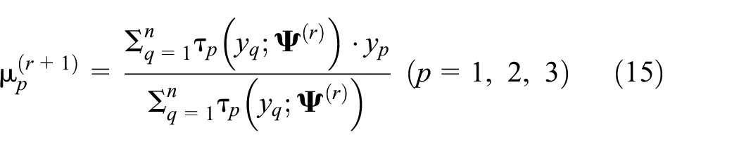
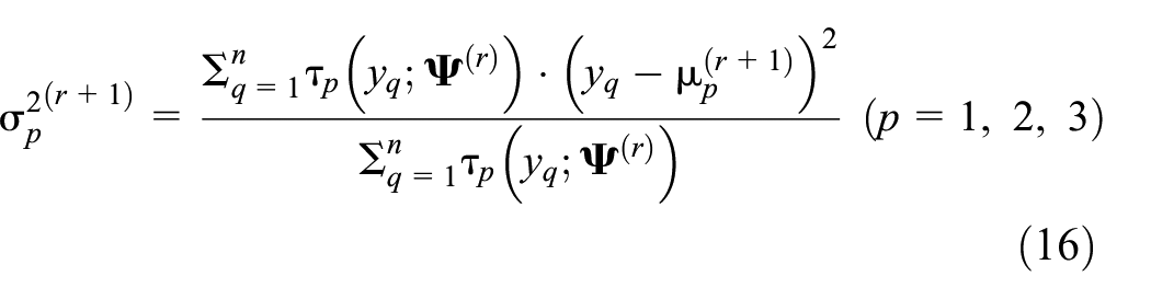
To obtain the updated estimator $Ψ^{(r + 1)}$ on the (r+1)th iteration, Equation (2) has to be solved as maximizing $Q (Ψ; Ψ^{(r)})$ . As the (r+1)th E-step returns the updated $z_{pq}$ with $τ_{p} (y_{q}; Ψ^{(r)})$ , the mixing portions in Equation (4) should be updated as follows:

\begin{matrix} π_{p}^{(r + 1)} = \frac{Σ_{q = 1}^{n} τ_{p} (y_{q}; Ψ^{(r)})}{n} (p = 1, 2, 3) \end{matrix}

(14)

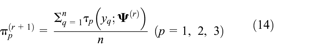
After substituting the expression of the normal distribution, Equations (5) and (6) can be solved explicitly at the (r+1)th iteration ( 32 ):

\begin{matrix} μ_{p}^{(r + 1)} = \frac{Σ_{q = 1}^{n} τ_{p} (y_{q}; Ψ^{(r)}) \cdot y_{p}}{Σ_{q = 1}^{n} τ_{p} (y_{q}; Ψ^{(r)})} (p = 1, 2, 3) \end{matrix}

(15)

\begin{matrix} {σ_{p}^{2}}^{(r + 1)} = \frac{Σ_{q = 1}^{n} τ_{p} (y_{q}; Ψ^{(r)}) \cdot {(y_{q} - μ_{p}^{(r + 1)})}^{2}}{Σ_{q = 1}^{n} τ_{p} (y_{q}; Ψ^{(r)})} (p = 1, 2, 3) \end{matrix}

(16)

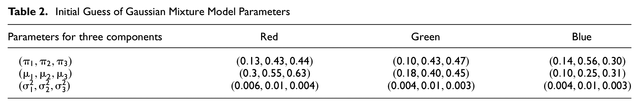
The EM iterations stop as the difference of the incomplete likelihood function $L (Ψ^{(r + 1)}) - L (Ψ^{(r)})$ reaches an arbitrarily small value, and the value of $L (Ψ^{(r)})$ is monotonically non-decreasing for $r = 0, 1, 2, \dots$ ( 33 ). This ensures the local convergence and a local maximum of $L (Ψ)$ with the local maximum likelihood estimator, $\hat{Ψ}$ . As the EM algorithm is affected by the initial guess of $Ψ$ , Table 2 gives the initial guess of $Ψ$ .

Table 2.

Initial Guess of Gaussian Mixture Model Parameters

Parameters for three components	Red	Green	Blue
$(π_{1}, π_{2}, π_{3})$	$(0.13, 0.43, 0.44)$	$(0.10, 0.43, 0.47)$	$(0.14, 0.56, 0.30)$
$(μ_{1}, μ_{2}, μ_{3})$	$(0.3, 0.55, 0.63)$	$(0.18, 0.40, 0.45)$	$(0.10, 0.25, 0.31)$
$(σ_{1}^{2}, σ_{2}^{2}, σ_{3}^{2})$	$(0.006, 0.01, 0.004)$	$(0.004, 0.01, 0.003)$	$(0.004, 0.01, 0.003)$

Point Estimation

Another way to determine the parameter vector $Ψ$ is by point estimation. The mean and variance of a GMM in Equation (1) can be calculated from the components’:

\begin{matrix} \bar{μ} = Σ_{p = 1}^{3} π_{p} μ_{p} \end{matrix}

(17)

and

\begin{matrix} \bar{σ^{2}} = Σ_{p = 1}^{3} π_{p} [σ_{p}^{2} + {(\bar{μ} - μ_{p})}^{2}] \end{matrix}

(18)

As discussed earlier, the parameter vector $Ψ$ for a single GMM has eight unknown values. To solve for these unknowns, at least eight equations are required. Each picture has three color channels, and each color channel has its own mean, $μ_{ijkl}$ , and variance, $σ_{ijkl}^{2}$ , with the subscript representing the ordinal of FI, picture sequence, color channel, and component, respectively. If each of the 36 pictures listed in Table 1 has its own GMM distribution, there are $36 \times 8 = 288$ unknown parameters. For all $6 \times 6 \times 3 = 108$ color channels listed in Table 1, a total of 216 equations need to be satisfied:

\begin{matrix} {\begin{matrix} {\bar{μ}}_{ijk} = Σ_{l = 1}^{3} π_{ijkl} μ_{ijkl} \\ {\bar{σ^{2}}}_{ijk} = Σ_{l = 1}^{3} π_{ijkl} [σ_{ijkl}^{2} + {({\bar{μ}}_{ijk} - μ_{ijkl})}^{2}] \end{matrix}, i = 1, 2, 3, 4, 5, 6; j = 1, 2, 3, 4, 5, 6; k = 1, 2, 3 \end{matrix}

(19)

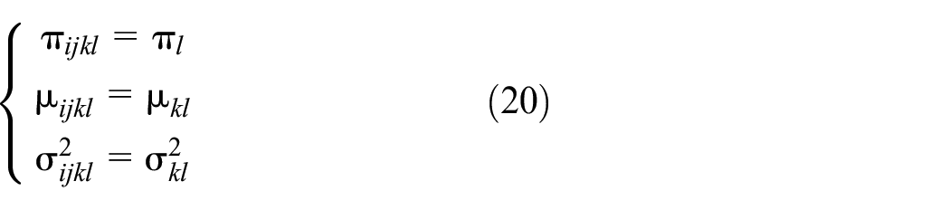
Obviously, the unknown parameters outnumber the equations. Noticing the ranges and their corresponding patterns in Figure 2, the first assumption is that:

The portion vector, $π = {(π_{1}, π_{2}, π_{3})}^{T}$ , is independent of the color channel.

Because all six pictures under one FI are the realizations of this FI, their GMM parameters are all estimations of the GMM parameters of this FI. The second assumption is that:

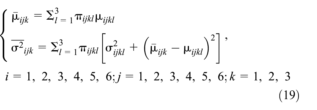
The parameter vector, $Ψ = {(π_{1}, π_{2}, μ^{T}, {σ^{2}}^{T})}^{T}$ , is independent of the picture sequence.

Before making more assumptions about the FI value, the following equations hold for one FI, subscript i, based on the two assumptions:

\begin{matrix} {\begin{matrix} π_{ijkl} = π_{l} \\ μ_{ijkl} = μ_{kl} \\ σ_{ijkl}^{2} = σ_{kl}^{2} \end{matrix} \end{matrix}

(20)

Substituting Equations (20) into Equations (19) yields the following equations for one FI, subscript i:

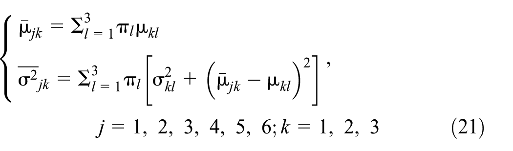
\begin{matrix} {\begin{matrix} {\bar{μ}}_{jk} = Σ_{l = 1}^{3} π_{l} μ_{kl} \\ {\bar{σ^{2}}}_{jk} = Σ_{l = 1}^{3} π_{l} [σ_{kl}^{2} + {({\bar{μ}}_{jk} - μ_{kl})}^{2}] \end{matrix}, j = 1, 2, 3, 4, 5, 6; k = 1, 2, 3 \end{matrix}

(21)

Equations (21) have 36 equations and 20 unknowns, making this system of equations possible to be solved or fitted.

Each equation in Equations (21) should have a residual $r_{jk}$ , and the summation of the squared residuals can be the objective function, which should be minimized over the parameter vector $Ψ$ :

\begin{matrix} min_{Ψ} {| | r_{jk} (Ψ) | |}^{2} = min_{Ψ} (Σ_{j = 1}^{6} Σ_{k = 1}^{3} r_{jk}^{2}) \end{matrix}

(22)

This non-linear fitting problem is solved by lsqnonlin function of MATLAB ( 34 ). The initial guess of parameters is the same as those in Table 2, and the absolute tolerance for each residual $r_{jk}$ is $10^{- 7}$ .

Results and Discussion

EM Fitting

For each color channel of the color triplet (R, G, B), the relative frequency is plotted against its corresponding color triplet component in Figure 3, and all the subplots share the common horizontal and vertical labels. Figure 3a demonstrates the GMM fitting of the relative frequency distribution of the Red channel. The green blocks constitute the relative frequency histogram of the Red channel, reflecting the statistical analysis of the fouled ballast image. The prominent curve represents the GMM distribution, while the three thinner curves correspond to the three GMM components. The three dashed vertical lines indicate the mean value for each component. While mixing proportions are not explicitly presented, the area under each thin curve corresponds to its mixing portion. Figure 3b and c , displays the fitting results for the Green and Blue channels, respectively.

Figure 3.

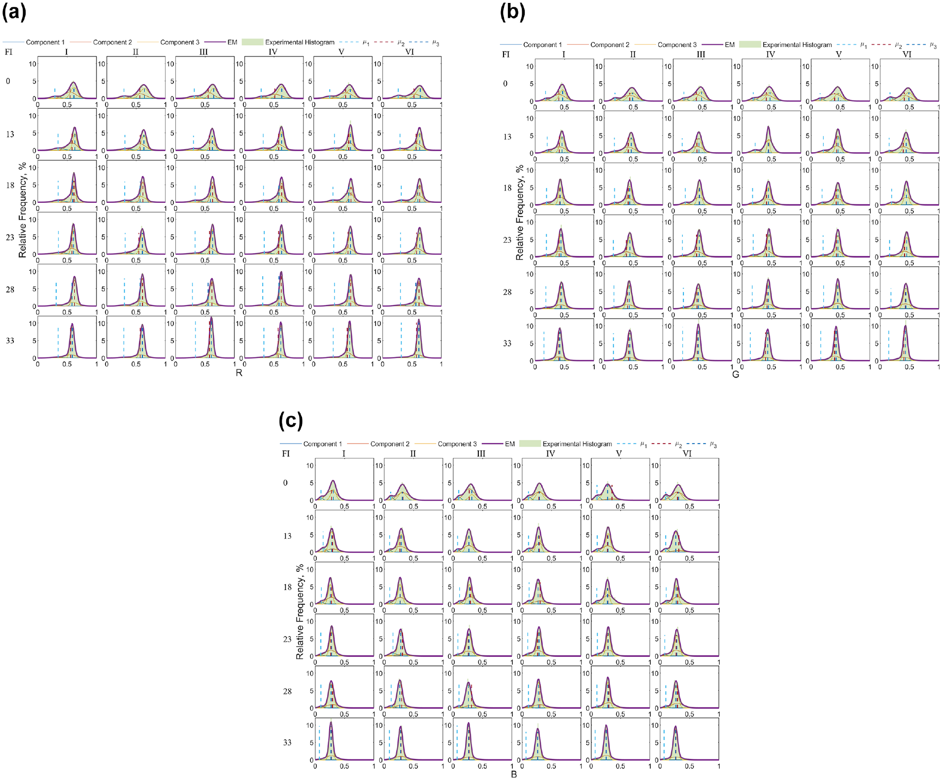
Expectation-maximization (EM) fitting results of all color intensity distributions in Table 1: color channels of the color triplet red (R), green (G), and blue (B): (a) red; (b) green; and (c) blue.

As the FI increases, whatever the channel, the first component, symbolizing voids, occupies a smaller proportion. The highest peak, comprised of the other two components, escalates as more areas of clustered fines appear in the fouled ballast. The fouled ballast histogram transitions from a two-peak curve to a one-peak curve, signifying a decrease in population variance with the rising peak height.

With a few exceptions, such as Figure 3b (FI 18-VI) and Figure 3c (FI 0-V), the sequence of the three components remains unchanged. There are more anomalous fittings in Figure 3c compared with Figure 3a or b , mainly because the mean value of the Blue intensity is lower than the other two, making it more challenging to successfully classify the three components.

Examining the position of these vertical lines under a single FI, slight variations in precise positions across different subplots can be observed, as each fouled ballast image represents a realization of its FI. These minor discrepancies indicate that the second assumption holds for both the portions and the mean values.

Averaged EM Parameters and Point-Estimated Parameters

Although the estimated parameters in Figure 3 do not precisely follow two assumptions, taking the average over these EM fitting parameters can obtain representative values for one FI, subscript i:

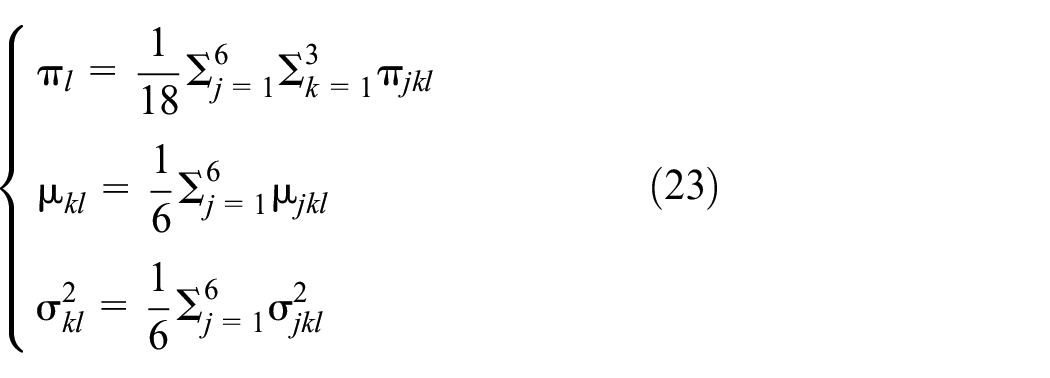
\begin{matrix} {\begin{matrix} π_{l} = \frac{1}{18} Σ_{j = 1}^{6} Σ_{k = 1}^{3} π_{jkl} \\ μ_{kl} = \frac{1}{6} Σ_{j = 1}^{6} μ_{jkl} \\ σ_{kl}^{2} = \frac{1}{6} Σ_{j = 1}^{6} σ_{jkl}^{2} \end{matrix} \end{matrix}

(23)

Therefore, these averaged EM-estimated parameters can be compared with those from point estimation.

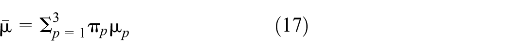
Figure 4 shows the mean values of GMM components in relation to the FI, with the two methods producing distinct trends. The average $μ_{kl}$ value for any component derived from the expectation-maximization (EM) method remains relatively stable, while the point estimate for the first component, $μ_{kl}$ , exhibits a positive correlation with the FI. If the mean values of the components consistently represent quantities of the fouled ballast, the following hypothesis can be proposed:

The mean vector, $μ = {(μ_{1}, μ_{2}, μ_{3})}^{T}$ , is independent of the FI.

Figure 4.

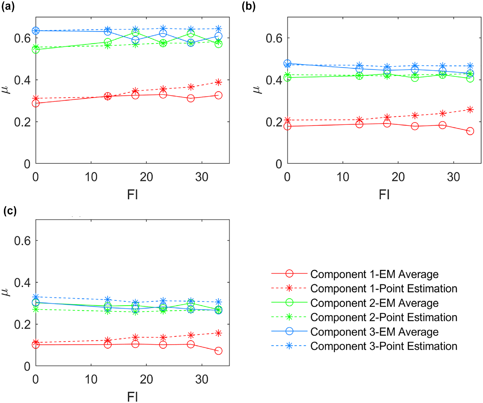
Component mean value estimation: (a) red channel; (b) green channel; and (c) blue channel.

Figure 5 illustrates the variance values of the GMM components in relation to the FI. The average variances determined through the EM method exhibit a gradual decrease in relation to the FI, whereas those computed through point estimation demonstrate more variability. Given that the component variance $σ_{kl}^{2}$ represents the inherent variability of fouled ballast components, such as the voids, a second hypothesis can be proposed:

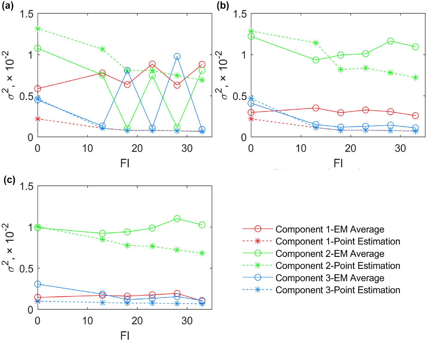
2. The variance vector, $σ^{2} = {(σ_{1}^{2}, σ_{2}^{2}, σ_{3}^{2})}^{T}$ , is independent of the FI.

Figure 5.

Component variance value estimation: (a) red channel; (b) green channel; and (c) blue channel.

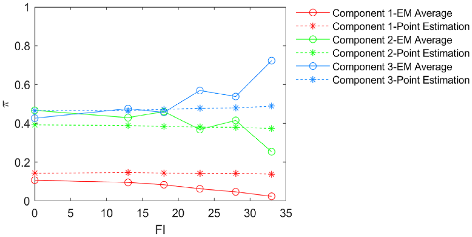
Figure 6 illustrates the relationship between the mixing portions and the FI. Instinctively, the mixing portion should represent the area of a component. Therefore, a fouled ballast image with a higher FI value should exhibit fewer visible voids, leading to a smaller mixing portion for the first component, $π_{1}$ . However, the mixing portions obtained through point estimation do not exhibit a strong correlation with the FI.

Figure 6.

Component mixing portion value estimation.

Obviously, differences in parameter estimation between the two methods are present. Given that higher-order moments are expected to yield less accurate estimations, particularly for non-normal distributions, it is worth noting that the point estimation method implemented here involves the second moment, the sample variance. The objective function in Equation (22) does not directly quantify the GMM fitting. As this equation represents the sum of squared residuals for each equation in Equations (21), it applies equal weight to each equation. However, considering that the absolute value of the mean is generally larger than the absolute value of the variance, the precision of variance estimation is effectively diminished.

Backcalculated Sample Parameters

The sample mean value can be backcalculated with Equation (17). Figure 7 shows the experimental, EM-estimated, and point-estimated sample mean values. Both backcalculated mean values fit the laboratory sieve analysis results well.

Figure 7.

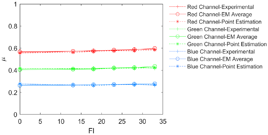
Comparison of sample mean value.

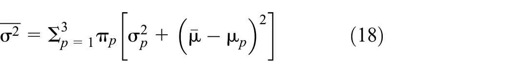
The sample variance value can be backcalculated using Equation (18). Figure 8 illustrates the experimental, EM-estimated, and point-estimated variances. Compared with the performance of sample mean backcalculation, it is more challenging to accurately fit the sample variances. The linear relationship between these two quantities is intriguing because the FI can be linearly predicted by the experimental sample variance ( 24 ). Nine sets of data from the three methods presented in Figure 8 are each used separately to fit the following linear regression equation:

F I_{k} = a_{k} σ_{k}^{2} + b_{k}, k = 1, 2, 3

(24)

Figure 8.

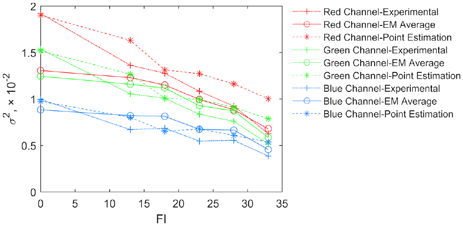
Comparison of sample variance value.

After conducting the linear regression fitting, the values of slope a, intercept b, and the indicator of fitting R² are listed in Table 3. The EM average method, having the smallest R² value, implies that its corresponding backcalculated sample variance has the least linear correlation with the FI.

Table 3.

Linear Fitting Results Between the FI and the Sample Variance

	Red	Green	Blue
	(Experimental, EM average, point estimation)
Slope a	(−2651, −4692, −3517)	(−3367, −4450, −4335)	(−5563, −6795, −7289)
Intercept b	(50.96, 68.00, 67.72)	(51.23, 62.98, 66.05)	(54.77, 68.03, 70.82)
R ²	(0.987, 0.880, 0.968)	(0.979, 0.834, 0.963)	(0.941, 0.805, 0.951)

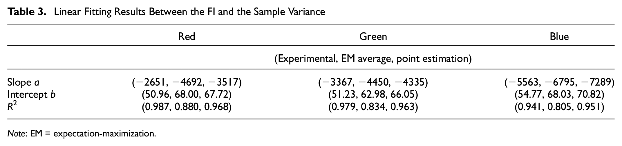
Note: EM = expectation-maximization.

Figure 9 presents the fitted data points alongside the linear regression lines. The discrepancies observed among different methods within a single color channel highlight that the experimental variance cannot be seamlessly merged with the backcalculated variance to establish a FI prediction model based on RGB variance. Compared with the experimental regression models, the other two sets of models show the discrepancy. The differences arise from the varied variance values for each FI value. When the experimental variance is directly calculated from the image channel intensity, the GMM backcalculated variances are from Equation (18). 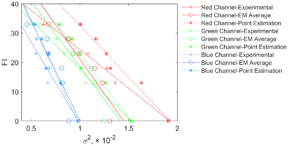The estimation of all the elements of the vector $Ψ = {(π_{1}, π_{2}, μ^{T}, {σ^{2}}^{T})}^{T}$ should vary with the estimation method, EM average, or point estimation.

Figure 9.

Linear regression between the sample variance and the FI.

Conclusions

As fouled ballast encompasses several elements, big ballast particles, clustered fines, and voids, this study attempts to decompose the RGB distributions of fouled ballast images into three components for each channel. The GMM was employed to classify these components, yielding fitting parameters such as component means, variances, and mixing proportions. Two estimation methodologies are used for these fitting parameters: expectation-maximization, which minimizes information loss by maximizing log-likelihood, and point estimation, which optimizes parameters by minimizing the sum of the squared residuals of the sample mean and variance expression. Based on these fitting outcomes, several notable conclusions can be drawn:

Both expectation-maximization and point estimation methods can estimate the GMM parameters given the assumptions, although discrepancies in values and the variations with FI differ.

Both methods demonstrate commendable performance when comparing the backcalculated sample means from various methods with the experimental sample means. However, with respect to sample variances, neither method accurately reproduces the backcalculated sample variances consistent with the experimental data.

A linear relationship between the sample variance and the FI is verified and explained, but the linear model may only apply to certain ranges.

Further research could implement data filtering and smoothing techniques to enhance data accuracy, and two conjectures on component properties are yet to be verified: 1) component means are independent of the FI; and 2) component variances are independent of the FI. Given the expression of sample variance, these GMM parameters can be represented in the form of the FI, thereby exploiting the GMM to characterize the fouled ballast more effectively.

Footnotes

Author Contributions

The authors confirm contribution to the paper as follows: study conception and design: Yufeng Gong, Yu Qian; data collection: Yufeng Gong; analysis and interpretation of results: Yufeng Gong, Yu Qian; draft manuscript preparation: Yufeng Gong, Yu Qian. All authors reviewed the results and approved the final version of the manuscript.

Declaration of Conflicting Interests

The author(s) declared no potential conflicts of interest with respect to the research, authorship, and/or publication of this article.

Funding

The author(s) disclosed receipt of the following financial support for the research, authorship, and/or publication of this article: This research is partially funded by the Federal Railroad Administration (FRA), Loram Maintenance of Way, Inc., M×V Rail, and BNSF Railway.

ORCID iDs

Yufeng Gong

Yu Qian

The opinions expressed in this article are solely those of the authors and do not represent the opinions of the funding agencies.

References

Jing

Qie

Markine

Jia

Polyurethane Reinforced Ballasted Track: Review, Innovation and Challenge. Construction and Building Materials, Vol. 208, 2019, pp. 734–748.

Hyslip

Sussmann

Chrismer

Railway Geotechnics. CRC Press, Boca Raton, FL, 2015.

Indraratna

Salim

Rujikiatkamjorn

Advanced Rail Geotechnology-Ballasted Track. CRC Press, Boca Raton, FL, 2011.

Sussmann

T. R.

Ruel

Chrismer

S. M.

Source of ballast fouling and influence considerations for condition assessment criteria. Transportation Research Record: Journal of the Transportation Research Board, 2012. 2289: 87–94.

Selig

E. T.

Waters

J. M.

Track Geotechnology and Substructure Management. Thomas Telford, London, 1994.

Kashani

H. F.

Hyslip

J. P.

C. L.

Laboratory Evaluation of Railroad Ballast Behavior Under Heavy Axle Load and High Traffic Conditions. Transportation Geotechnics, Vol. 11, 2017, pp. 69–81.

Kashani

H. F.

C. L.

Hyslip

J. P.

Fouling and Water Content Influence on the Ballast Deformation Properties. Construction and Building Materials, Vol. 190, 2018, pp. 881–895.

Tennakoon

Indraratna

Rujikiatkamjorn

Nimbalkar

Neville

The Role of Ballast-Fouling Characteristics on the Drainage Capacity of Rail Substructure. Geotechnical Testing Journal, Vol. 35, No. 4, 2012, pp. 629–640.

Huang

Tutumluer

Dombrow

Laboratory Characterization of Fouled Railroad Ballast Behavior. Transportation Research Record: Journal of the Transportation Research Board, 2009. 2117: 93–101.

10.

Wilk

S. T.

A Deep Investigation into the Mechanisms and Factors Producing Mud Pumping of Railway Track. Transportation Geotechnics, Vol. 38, 2023, p. 100908.

11.

Luo

Huang

Ding

Qamhia

I. I.

Tutumluer

Hart

J. M.

Thompson

Sussmann

T. R.

Toward Automated Field Ballast Condition Evaluation: Algorithm Development Using a Vision Transformer Framework. Transportation Research Record: Journal of the Transportation Research Board, 2023. 2677: 423–437.

12.

Indraratna

Ngo

N. T.

Rujikiatkamjorn

Deformation of Coal Fouled Ballast Stabilized with Geogrid Under Cyclic Load. Journal of Geotechnical and Geoenvironmental Engineering, Vol. 139, No. 8, 2013, pp. 1275–1289.

13.

Tutumluer

Ahuja

Hart

J. M.

Moaveni

Huang

Zhao

Shah

Field Evaluation of Ballast Fouling Conditions Using Machine Vision. Transportation Research Board, Washington, D.C., 2017.

14.

Sussmann

Jr. Thompson

II Stark

Wilk

Use of Seismic Surface Wave Testing to Assess Track Substructure Condition. Construction and Building Materials, Vol. 155, 2017, pp. 1250–1255.

15.

Stark

T. D.

Wilk

S. T.

Thompson

H. B.

Sussmann

T. R.

Jr. Baker

C. L.

Evaluating Fouled Ballast Using Seismic Surface Waves. Proc., 2016 Joint Rail Conference. 2016 Joint Rail Conference. Columbia, SC, 2016. V001T01A002. ASME. https://doi.org/10.1115/JRC2016-5714.

16.

Liu

Huang

Qiu

Gao

Comparison of Laboratory Testing Using Smartrock and Discrete Element Modeling of Ballast Particle Movement. Journal of Materials in Civil Engineering, Vol. 29, No. 3, 2017, p. D6016001.

17.

Huang

Liu

Qiu

Identification of Railroad Ballast Fouling Through Particle Movements. Journal of Geotechnical and Geoenvironmental Engineering, Vol. 144, No. 4, 2018, p. 02818001.

18.

Zeng

Qiu

Bian

Xiao

Huang

Identification of Ballast Condition Using SmartRock and Pattern Recognition. Construction and Building Materials, Vol. 221, 2019, pp. 50–59.

19.

Nazari

Huang

Qiu

Identification of Railroad Ballast Fouling Through Statistical Process Control on Ballast Particle Movement. Transportation Geotechnics, Vol. 36, 2022, p. 100780.

20.

Roberts

Rudy

Al-Qadi

Tutumluer

Boyle

Railroad Ballast Fouling Detection Using Ground Penetrating Radar–A New Approach Based on Scattering from Voids. Proc., Ninth European Conference on NDT, Berlin, Germany, Citeseer, 2006.

21.

Leng

Al-Qadi

I. L.

Railroad Ballast Evaluation Using Ground-Penetrating Radar: Laboratory Investigation and Field Validation. Transportation Research Record: Journal of the Transportation Research Board, 2010. 2159: 110–117.

22.

Hyslip

J. P.

Smith

S. S.

Olhoeft

G. R.

Selig

E. T.

Assessment of Railway Track Substructure Condition Using Ground Penetrating Radar. Proc., 2003 Annual Conference of AREMA, Chicago, Citeseer, 2003.

23.

Ichi

Dorafshan

Spectral Characterization of Fouled Railroad Ballast Using Hyperspectral Imaging. Construction and Building Materials, Vol. 394, 2023, p. 132076.

24.

Gong

Qian

Predicting Ballast Fouling Conditions Through RGB-Based Statistical Quantity Analysis. Transportation Research Record: Journal of the Transportation Research Board, 2024. 2678: 153–166.

25.

McLachlan

Peel

Finite Mixture Models. John Wiley & Sons, New York, NY, 2000.

26.

Wang

Zhao

Cao

Site-Specific Probability Distribution of Geotechnical Properties. Computers and Geotechnics, Vol. 70, 2015, pp. 159–168.

27.

Depina

T. M. H.

Eiksund

Strøm

Cone Penetration Data Classification with Bayesian Mixture Analysis. Georisk: Assessment and Management of Risk for Engineered Systems and Geohazards, Vol. 10, No. 1, 2016, pp. 27–41.

28.

Bouayad

Baroth

Dano

Gaussian Mixture Model Based Soil Classification Using Multiple Cone Penetration Tests. IOP Conference Series: Earth and Environmental Science, Vol. 696, 2021, p. 012034.

29.

Guan

Wang

Non-parametric Construction of Site-Specific Non-Gaussian Multivariate Joint Probability Distribution from Sparse Measurements. Structural Safety, Vol. 91, 2021, p. 102077.

30.

Sun

Zheng

Clone Granular Soils with Mixed Particle Morphological Characteristics by Integrating Spherical Harmonics with Gaussian Mixture Model, Expectation–Maximization, and Dirichlet Process. Acta Geotechnica, Vol. 15, No. 10, 2020, pp. 2779–2796.

31.

Deng

Q.-X.

Cao

Z.-J.

Papaioannou

D.-Q.

Phoon

K.-K.

Bayesian Learning of Gaussian Mixture Model for Calculating Debris Flow Exceedance Probability. Georisk: Assessment and Management of Risk for Engineered Systems and Geohazards, Vol. 16, No. 1, 2022, pp. 154–177.

32.

McLachlan

G. J.

Krishnan

The EM Algorithm and Extensions. John Wiley & Sons, Hoboken, NJ, 2007.

33.

Dempster

A. P.

Laird

N. M.

Rubin

D. B.

Maximum Likelihood from Incomplete Data via the EM Algorithm. Journal of the Royal Statistical Society: Series B (Methodological), Vol. 39, No. 1, 1977, pp. 1–22.

34.

The MathWorks Inc. MATLAB Version: 9.14.0.2206163 (R2023a). The MathWorks Inc., Natick, MA, 2023.

Predicting Ballast Fouling Conditions with the Gaussian Mixture Model

Abstract

Keywords

Fouled Ballast Image

Gaussian Mixture Model

Expectation-Maximization

E-Step

M-Step

Point Estimation

Results and Discussion

EM Fitting

Averaged EM Parameters and Point-Estimated Parameters

Backcalculated Sample Parameters

Conclusions

Footnotes

Author Contributions

Declaration of Conflicting Interests

Funding

ORCID iDs

References