
Abstract
Transportation infrastructure in Texas, U.S., particularly its extensive bridge network, plays a vital role in supporting economic growth and ensuring safe and efficient mobility. With over 57,000 bridges, including more than 22,000 culverts, Texas faces the challenge of maintaining its infrastructure while dealing with limited funding resources. This paper presents the findings of a study conducted for the Texas Department of Transportation that focused on assessing the costs associated with bridge consumption by oversize and overweight (OS/OW) vehicles. The study aimed to calculate bridge consumption costs per mile for different OS/OW categories, considering factors such as axle load, spacing, bridge design life, and vehicle miles traveled (VMT). These consumption costs were calculated by analyzing traffic data and bridge inventory ratings. The results showed that, although OS/OW vehicles are responsible for the majority of the bridge consumption costs per mile, their lower VMT, relative to regular commercial vehicles, mitigates their influence on total bridge consumption costs to less than 15% of the total. The findings of this study can contribute to the ongoing efforts of transportation engineers and policymakers in addressing funding deficits and developing strategies to sustain the state’s bridge infrastructure.
Transportation infrastructure plays a crucial role in facilitating the Texas, U.S., economy, ensuring the safe and efficient movement of people and goods across the state. Texas maintains the largest bridge inventory in the U.S.—about 57,000 bridge structures, which include over 22,000 culverts, with an overall deck area of about 539 million square feet—and achieves a level of safety where zero crashes are caused annually by poor bridge conditions. Texas’s bridges are mainly grouped in two categories: on-system and off-system bridges. The first one is located on state highway systems and funded by both state and federal agencies. The latter combines the rest of the bridges which are not located on state highway and are owned by local governments ( 1 ).
The primary funding source for bridge maintenance comes from a combination of federal and state resources. Federal funds are appropriated by Congress through the federal Highway Trust Fund while the State utilizes motor fuels tax, vehicle registration fees, sales taxes, and oil and gas production tax. Additionally, revenue from oversize and overweight (OS/OW) permits contributes to the state highway fund. However, reduced revenue associated with the rise of fuel-efficient/electric vehicles has further strained the already limited resources for road infrastructure maintenance. Transportation managers and legislators are focused on evaluating the road infrastructure consumption induced by OS/OW vehicles to bridge structures and the balancing of this consumption (in dollars/mile) to the revenue based on the permit fees.
Motor fuels tax revenue, vehicle registration fees, and OS/OW permit fees are all revenue sources that are tied to vehicle usage. The oil and gas (severance and sales) taxes are revenues that are used for transportation but are not typically referred to as user fees. The fuel tax as a funding mechanism is politically unreliable on the long term, since it is not indexed but set at a fixed rate. In addition, fuel efficiency is likely to increase more in the future, as average fuel economy standards ratchet up and alternative fuels become more cost-effective ( 2 ).
To address the potential for a growing budget deficit, the Texas legislature has conducted numerous studies to identify potential funding sources, determine the necessary increase in funding, and allocate the current budget effectively to maintain a satisfactory level of serviceability for both the road and bridge network. While OS/OW vehicles contribute more toward the maintenance needs of roads and bridges, they also serve as a significant economic driver within the state. Researchers and transportation engineers have suggested that adjusting the permitting fee structure for OS/OW vehicles would be a practical solution to address the funding deficit ( 3 ).
Past studies found that overweight (OW) corridors are seen as marketing tools for local agencies that promote economic development in their areas and that these agencies were working to expand their OW corridors. Companies operating with OW permits experience increased productivity and efficiency because permits eliminate the need to redistribute divisible loads on several vehicles to meet legal weight limits ( 4 , 5 ). Moreover, while pavement structures respond to axle loads and are relatively insensitive to spacing between axle groups, bridge structures respond to both axle loads and spacing. In Texas, the study found bridge consumption rates also varied based on whether a county was rural or urban, because of bridge density (bridges/mile). Truck configurations varied among OW corridors evaluated, which can particularly affect bridge consumption rates based on truck outer bridge lengths.
Road infrastructure consumption has been previously addressed on several studies, most of them related to pavement consumption since pavement fatigue concepts have been historically used. Bridge consumption calculations used a similar conceptual approach, in the sense that each passage of the OS/OW-permitted vehicle consumes a portion of the asset value of a given bridge ( 3 – 5 ). This bridge consumption theory is based on current bridge ratings and the force effects of the current bridge ratings and the OS/OW vehicle configuration, as summarized by its axle loads and axle spacings.
This paper summarizes the results published for the Texas Department of Transportation (TxDOT) “Study on motor vehicle impacts on road and bridges of Texas” which was conducted to assess the bridge consumption costs for the various vehicle classification that operate on Texas highways (including OS/OW vehicles) by calculating bridge consumption costs per mile ( 3 ). The methodology considered each vehicle configuration (axle load and spacing) and its respective effect based on load-passage as a fractional consumption of the bridge’s design life. The costs for externalities, such as the impacts of traffic delays caused by work zones and detours to upgrade bridges because of commercial traffic operations, were not considered.
Bridge Consumption Analysis
The first studies on bridge consumption were based on the American Association of State Highway and Transportation Officials (AASHTO) bridge design guide, which incorporates fatigue curves to quantify the number of stress cycles experienced by a bridge throughout its design life ( 6 ). This set of curves are for steel elements, but, by implementing standard fatigue modeling equations, that may be extended to other materials with the appropriate material testing ( 7 – 9 ). The wider the stress range, the lower the number of stress cycles to get to the end of the design life of a specific structural detail. The design guide specifies a lifespan of 75 year or 2 million applications of the design load HS20-44, shown in Figure 1.
Standard bridge design load HS20-44.
A previous federal highway cost allocation study attributed 11% of the bridge asset value to loads that are over HS20-44 ( 10 ). Bridge inventory ratings in Texas are continuously updated to reflect bridge deterioration and are also recorded as multiples of the HS20-44. Thus, the bridge model used in this study adapted from the fatigue concept is presented in Equation 1.

where
BC = the bridge consumption for the vehicle configuration analyzed,
DA = the bridge deck area in square feet,
AV = the asset value for a bridge in dollars per bridge deck square foot,
0.11 = a coefficient: the bridge asset value responsibility for heavy trucks,
MTRAFFIC = the live load bending moment truck configuration being analyzed for each bridge,
MINVENTORY = the live load bending moment for the inventory rating load for each bridge analyzed,
m = a constant (material dependent), and
2,000,000 = a constant: the number of allowable load cycles that define the bridge design life, according to AASHTO.
This equation represents the consumption in dollars caused by the passage of one specific truck configuration over a given bridge on a specific route.
The inventory rating load is the live load that can safely utilize the bridge for an indefinite period of time. This load causes stresses equivalent to those caused by the design load, but reflects the current load rating for a given bridge ( 11 ). The computer program Moment Analysis of Structures (MOANSTR), which uses a finite-difference routine, was then used to calculate the maximum live load moments for the OS/OW load (MTRAFFIC) in Equation 1, and the bridge inventory load for a specific bridge (MINVENTORY) in Equation 1 ( 12 ). The moment ratios in Equation 1 are calculated for every bridge in the inventory, using the “m” value for its material type, retrieved from the bridge inventory database. Every bridge is then associated to the different road segments using a geographic information system (GIS)-based procedure, and bridge consumption costs are accumulated for each GIS road segment to calculate bridge consumption costs per mile, using Equation 1.
OS/OW Vehicle Miles Traveled (VMT)
As mentioned earlier, this study focusses on OS/OW vehicles because of the unique impact these vehicles have on bridge consumption by presenting a greater bridge consumption in relation to wear and tear. Texas has size and weight limits for vehicles traveling on its roads and bridges. If a vehicle is over the size or weight limit, a permit is required to travel. The OS/OW permits are either routed or non-routed. Routed permits are single-use and must designate the specific route of travel, while non-routed permits vary and can be used multiple times, in multiple locations, and, in some instances, by multiple trucks. Thus, the type of permit dictates the travel parameters and the associated bridge consumption analysis procedure.
To calculate the OS/OW vehicle miles traveled (VMT), researchers first applied estimated annual mileage assumptions to specific permit types. These mileage assumptions were based on discussions with Texas Department of Motor Vehicles (TxDMV), which is the entity responsible for tracking and assessing fees on registered motor vehicles in Texas. Researchers identified the VMT associated with routed permits using data from TxDMV’s Texas Permitting and Routing Optimization System (TxPROS). The routed VMT was divided between OS and OW based on the total estimated VMT of mileage for specific OS/OW permits described in Table 1. Each permit category was summarized by several axle and spacing load configurations.
Estimated Vehicle Miles Traveled (VMT) by Oversize and Overweight Permit Type
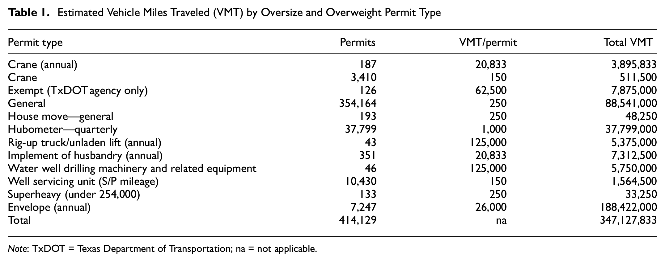
Note: TxDOT = Texas Department of Transportation; na = not applicable.
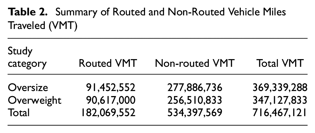
The remaining OS/OW VMT is attributed to the non-routed permit travel, as summarized in Table 2. These permits can vary by time, allowing a single permit to be reused for multiple trips annually, quarterly, or for 30, 60, or 90 days. Additionally, these permits can vary by location and allow for travel either within a set group of counties, or statewide. Multiple variations allow for greater flexibility when moving certain types of OS/OW loads. The routed and non-routed OS/OW VMT were disaggregated based on the percentage of permits defined as either oversized (OS) (52%) or OW (48%).
Summary of Routed and Non-Routed Vehicle Miles Traveled (VMT)
Results and Discussions
The permitting information for OS/OW trucks was provided by TxDMV. Data from 2019 were selected to avoid the unusual traffic patterns which resulted from the COVID-19 pandemic. The OS/OW permit database contained 429,667 records. A data analysis indicated that only 56 (0.01%) of these permits did not have complete information, because of missing data either for the spacing between the axles or for the weight of the axle. Given the negligible amount of missing data, those entries were removed from the database to avoid any issues related to uncertainty. The number of observations in the database after removing these incomplete records totaled 429,611.
OS/OW Vehicle Characterization
First, the frequency distribution for the number of axles per OS/OW vehicle was obtained to determine which axle counts are most commonly observed among the granted permits. Next, the number of axle groups per vehicle was determined by using the definition from the Texas Transportation Code: “…two or more consecutive axles spaced 40 inches and not more than 96 inches apart…” ( 13 ). The data indicate that most OS/OW trucks have between five and nine axles; approximately one in four OS/OW vehicle permits has eight axles, the most common arrangement. Moreover, those OS/OW vehicles that were granted a permit had two to five axle groups, with a little over 70% of all trucks having three axle groups, as depicted in Figure 2. Number of axles and axle groups were determined following the definitions from the Texas Transportation Code.
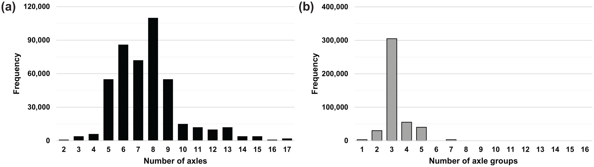
Distribution of: (a) number of axles and (b) number of axle groups.
The data information was then combined to obtain the axle configurations for the OS/OW vehicles (Table 3). In this study, the various vehicle configurations are labeled to indicate how many axle groups a vehicle has and, within each of those axle groups, how many axles are present. The labels are formatted using numbers and dashes, with the number of axles present in each axle group separated by dashes, going from the front of the vehicle to the end of the last trailer.
Tabulation of the 27 Most Common Oversize and Overweight Vehicles
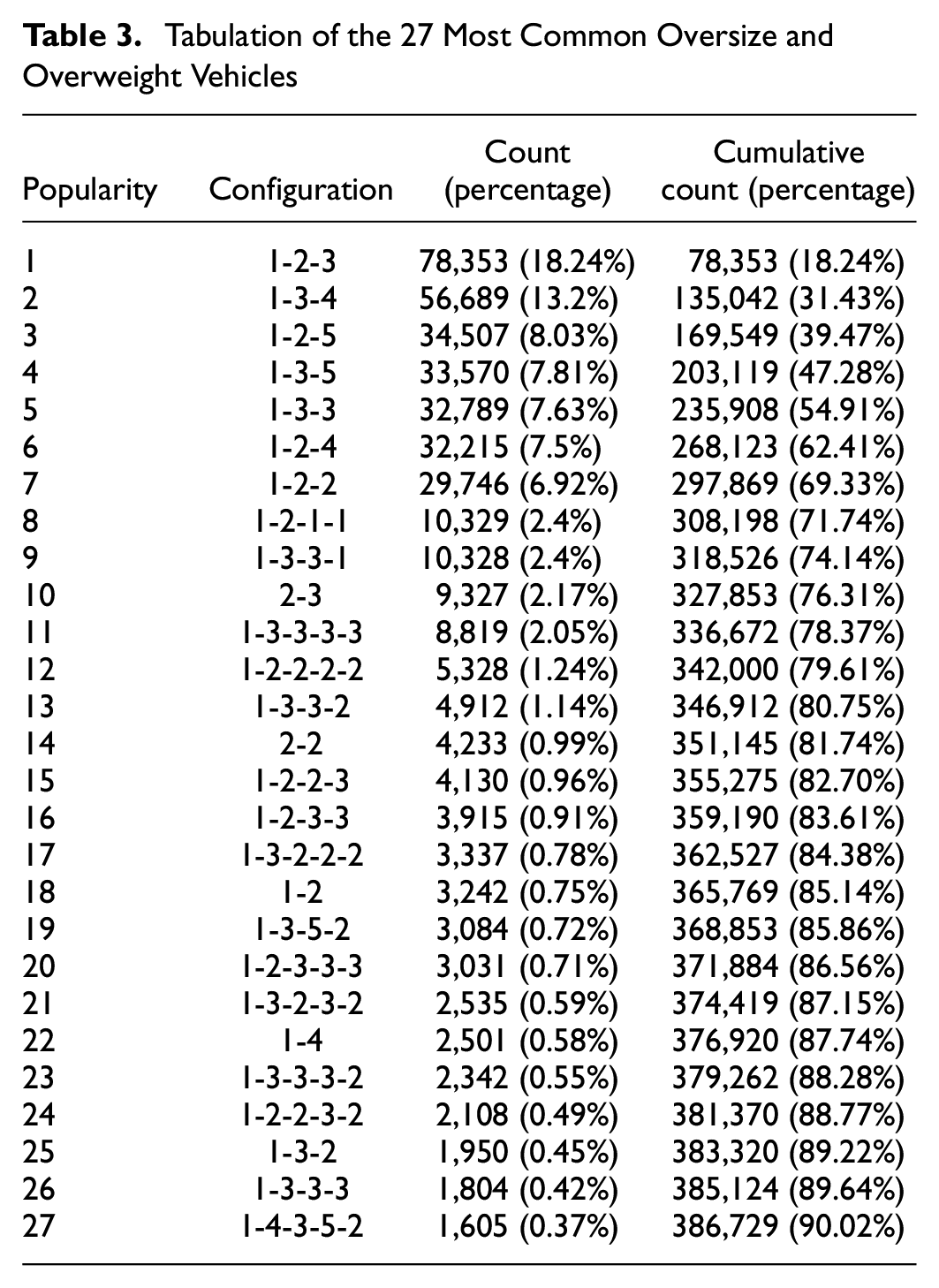
In concert with TxDOT, it was decided to use the 2019 Central Permit Office Axle and Base Report files to determine the representative configurations for the different permit types. To better explain the methodology application, a detailed analysis for the case of 80 to 120 kip permitted vehicles is presented. Note that vehicles with Gross Vehicle Weight (GVW) exceeding 254,300 lb were not included in the analysis.
The distribution of number of GVW for the 80 to 120 kip GVW category is shown in Figure 3. The most frequent number of axles was six, followed by seven, whereas the most frequent GVW (31.3%) was 120 kip.
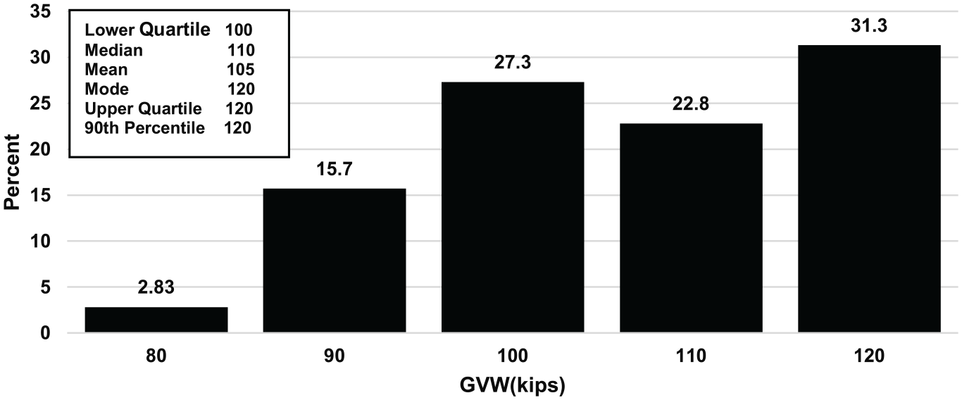
Distribution of GVW for the 80 to 120 Gross Vehicle Weight (GVW) category.
Results of the statistical analyses indicate that the typical steering axle is a single axle weighing 14 kip. The data showed that 99.94% of first axles have two tires, and the most frequent spacing is 18 ft (Figure 4).
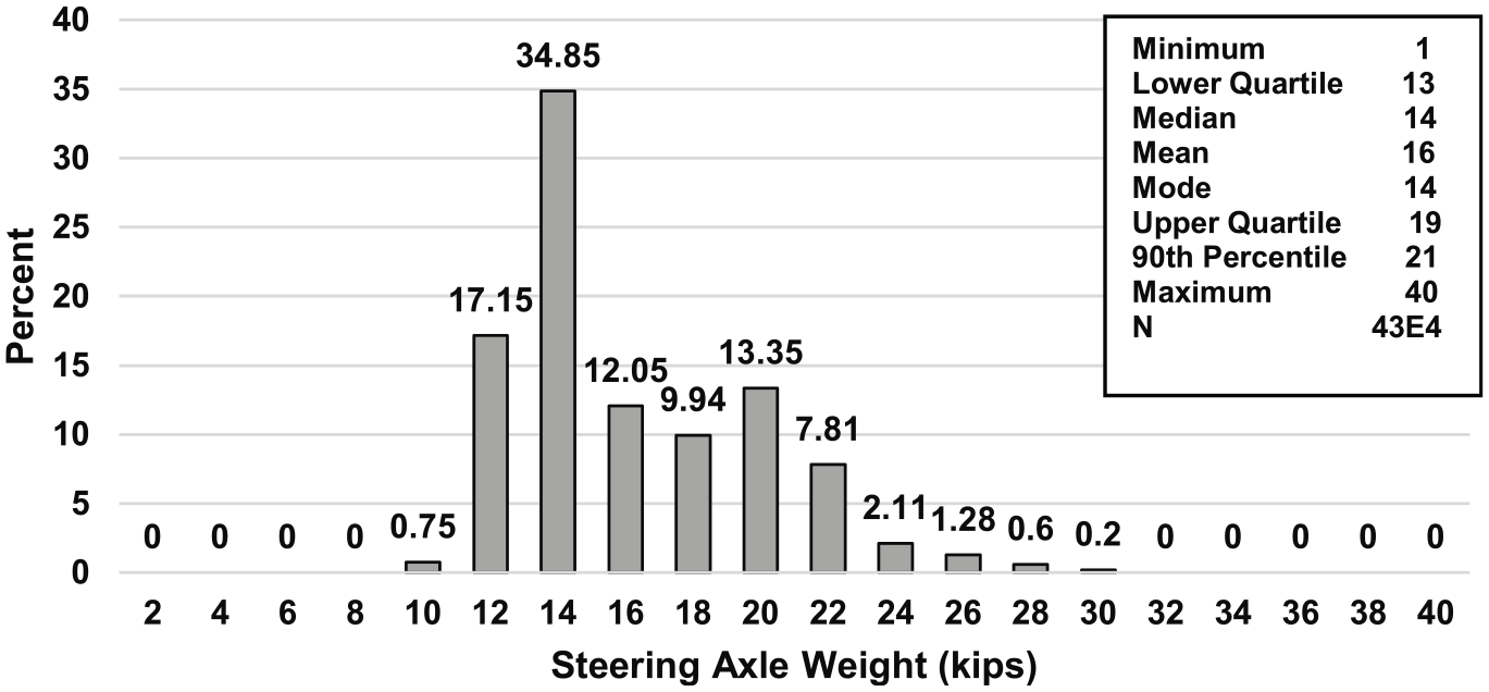
Steering axle weight distribution, 80 to 120 kip Gross Vehicle Weight (GVW) category.
The most frequent steering axle weight was 14 kip. For the tractor rear, the spacing between the steering and the first tractor axle fitted a uniform distribution around 5 ft. Thus, the tractor rear axle was multiple. Spacing within the tractor axles indicated that, although a tridem rear axle was present rather frequently, the axle weight data showed that the second and third axle weights had quite similar distributions, while the weight of the fourth axle was different. Therefore, the typical rear tractor axle was a tandem. Finally, according to Figure 3, the most frequent GVW is fully loaded (120,000 lb), which is also confirmed by the mode of the tractor axles.
Figure 5 shows the distribution of the space between the third and fourth axles. The axle spacing distribution indicates that nearly 80% of the tractors had tandem rear axles. The mean spacing of this subset was 39 ft, and the mode was 32 ft. The most frequent spacing in the entire category within the subset was 36 ft. Therefore, the best value for the space between the tractor axle and the trailer was 35 ft. The data also indicated that the trailer axle was a tridem axle weight mode of 20 kip.
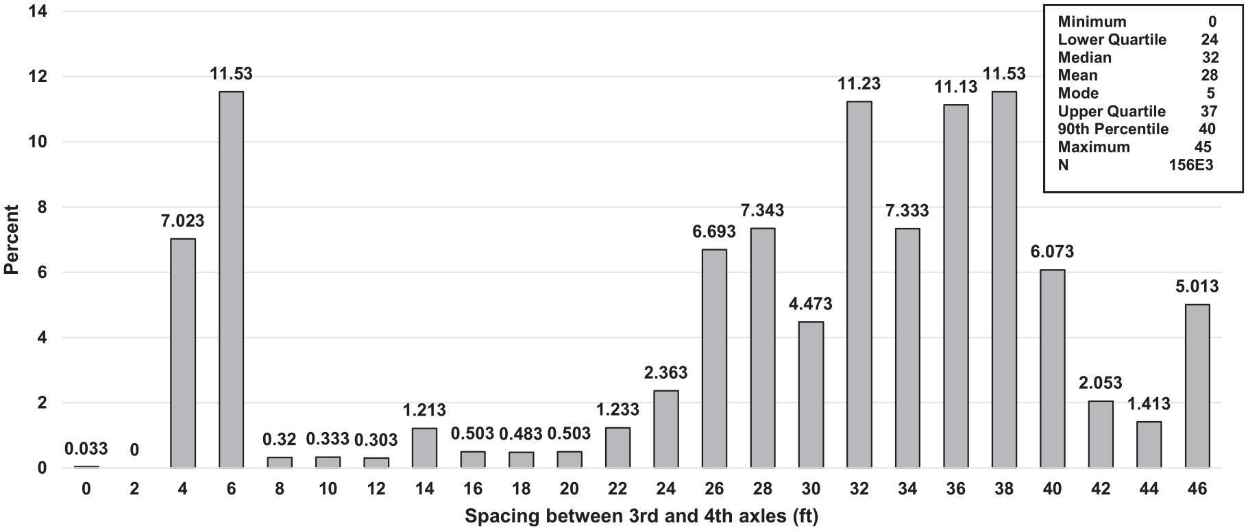
Spacing between third and fourth axles, 80 to 120 kip Gross Vehicle Weight (GVW) category.
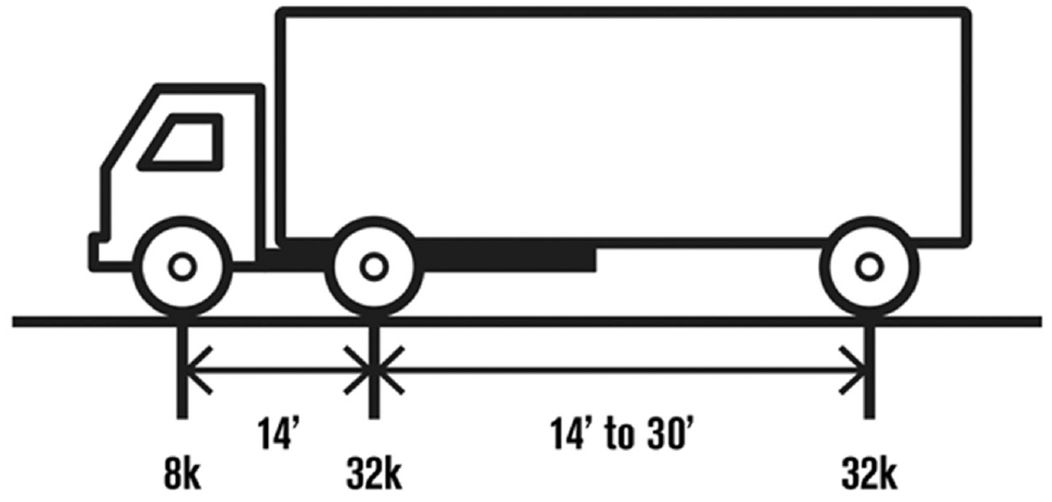
If no tentative configuration can be determined from the overall data, there is more than one representative configuration in that GVW category. In this case, this step must be repeated by the number of axles, permit type, or both, until representative configurations are satisfactory. This was necessary for heavier categories but not for the case presented here. Therefore, the data indicated one configuration for the 80 to 120 kip category, which is depicted in Figure 6.
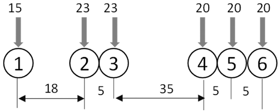
Gross Vehicle Weight (GVW) category: 80,001 to 120,000 lb (loads in kip and spacing in feet).
Bridge Consumption
The bridge analysis methodology relied on the readily available data sources maintained by TxDOT: the bridge inventory database (TxDOT Bridges) and the road inventory database (TxDOT Road Inventory) ( 11 , 14 ). Then, using both inventories, the bridge data were merged to all routes in a GIS platform. Combining the routes and the representative configurations of OS/OW vehicles, the bridges on all routes were retrieved and the necessary variables for the consumption analysis were calculated, leading then to a bridge consumption cost per mile for each configuration. The analysis for the 80 to 120 kip GVW category is presented to illustrate the bridge consumption concepts.
GIS Database Preparation
The TxDOT Roadway Inventory was downloaded from TxDOT’s publicly available data ( 14 ). The roadway data were then loaded in ESRI’s ArcGIS Pro and processed to include only the road alignments, excluding the frontage road system also present in the raw GIS TxDOT roadway data. After this data processing, the resulting alignments were re-segmented to provide road segments approximately 10 mi long. The next step in the GIS data preparation consisted of loading the georeferenced bridge inventory database, TxDOT Bridges, on ArcGIS Pro to start the initial geoprocessing of assigning the bridges in the TxDOT Bridges file to roadway data ( 14 ). The resulting spatial intersection of the bridge and roadway data was then downloaded, and SAS™ programs were developed for further data cleanup, including, but not restricted to, filtering out bridge duplicates generated by the geoprocessing step to spatially merge both bridge and roadway files. This interactive process results in a finalized bridge/roadway database that is the basis for the bridge consumption analysis required by this study.
A 10.9 mi roadway segment of IH 35 northbound near Dallas, containing 23 bridges, is depicted in Figure 7, this is used to illustrate the finalized combined bridge road segment GIS database.
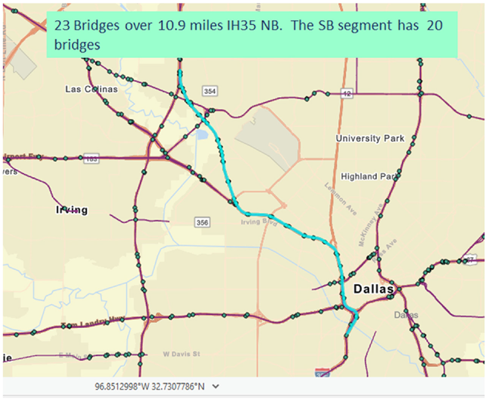
Bridge and roadways geographical information systems (GIS) segments.
The computer program MOANSTR was then used to calculate the live load moments in Equation 1 for every bridge recorded in the GIS database previously discussed. The MOANSTR program’s core is a finite-differences routine that calculates the live load moment envelopes generated by the vehicle configurations developed for the consumption analysis, and by the inventory rating loads also recorded in the GIS database prepared for this bridge consumption analysis.
The bridge consumption (in dollars) resulting from a given load pass was estimated by combining the results obtained with a consumable asset value for the bridges. Research developed in support of the Texas 2030 Committee established that the asset value of a bridge was $190/sq ft of deck area in 2008 dollars ( 15 ). Updating these values for 2021, when this HB2223 project was developed, using the Federal Highway Administration (FHWA) National Highway Construction Cost Index resulted in $236/sq ft ( 16 ).
Monte Carlo Simulation
The GIS segments of the previously described database were randomly sampled using a Monte Carlo simulation. This randomly sampled road segments approach was included in the modeling to more closely represent the random routes that the OS/OW vehicles may take when using the purchased permits. The OS/OW permits for this study are not classified as super heavy loads; those have to follow a pre-determined road route. Each randomly sampled segment contains a certain number of bridges and has a certain length, which is close to 10 mi, as discussed previously. Each randomly sampled set of segments must represent an annual mileage for each specific vehicle configuration. Therefore, it was necessary to run sensitivity analyses of the bridge consumption cost per mile versus annual mileage. The results indicated that the bridge consumption cost per mile was not sensitive to annual mileages above 20,000 mi, since this mileage in relation to GIS segments selected by the Monte Carlo simulation was enough to represent the random routes of a specific permit on the Texas road network.
After establishing this random GIS segment data set using a computerized SAS™ routine, the analysis followed steps that consisted of aggregating the data generated by the bending moment analysis with the GIS bridge and segment data. Bending moments for the traffic configuration and inventory rating loads were calculated using the MOANSTR computerized routine, and results for Equation 1 were calculated for all bridges identified in the randomly assigned GIS segments to determine bridge consumption. Finally, results were aggregated for mileage and bridge consumption, allowing for the calculation of bridge consumption costs per mile.
Because the routes were not fixed for this type of OS/OW permit, segments were randomly assigned to fulfill the established >20,000 mi of random route segments for each representative traffic configuration. Bridge density (bridge count by GIS segment) was also relevant to these calculations. Statistical analyses of bridge count per mile showed a significant difference in bridge density for East and West Texas counties. To properly consider this issue, the analysis was done separately for East and West Texas counties, as depicted in Figure 8.
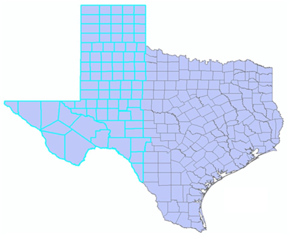
Segregation of bridge consumption calculation into East and West Texas, Black outlined counties are in East Texas.
The cost per mile was found to be higher for the eastern counties than for the western counties; the bridge densities per mile for the eastern counties were much higher since eastern counties in Texas are more urbanized, as presented in Table 4. In addition, Table 4 shows that four random runs of the consumption analysis were performed to calculate an average bridge consumption cost per mile.
Example Analysis of Bridge Consumption for Eastern and Western Counties (80 to 120 kip Configuration)
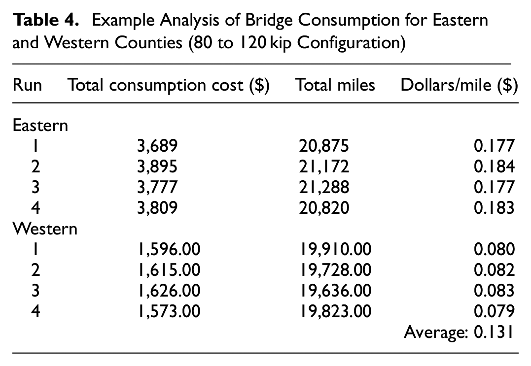
The final results from the random runs were averaged and the bridge consumption costs for eastern counties were 18 cents/mile, and for western counties were 8 cents/mile, resulting in an overall average of 13 cents/mile for the 80 to 120 kip GVW category. The results of the random runs clearly showed that the segments were randomly selected to complete the targeted 20,000 mi of annual travel for the OS/OW configuration.
The results for all the vehicles categories are presented in Table 5, including both commercials and OW vehicles for comparison purposes. An interesting observation is that over 80% of the estimated bridge consumption costs are under $ 0.25/mile.
Bridge Consumptions Costs for Each Vehicle Category
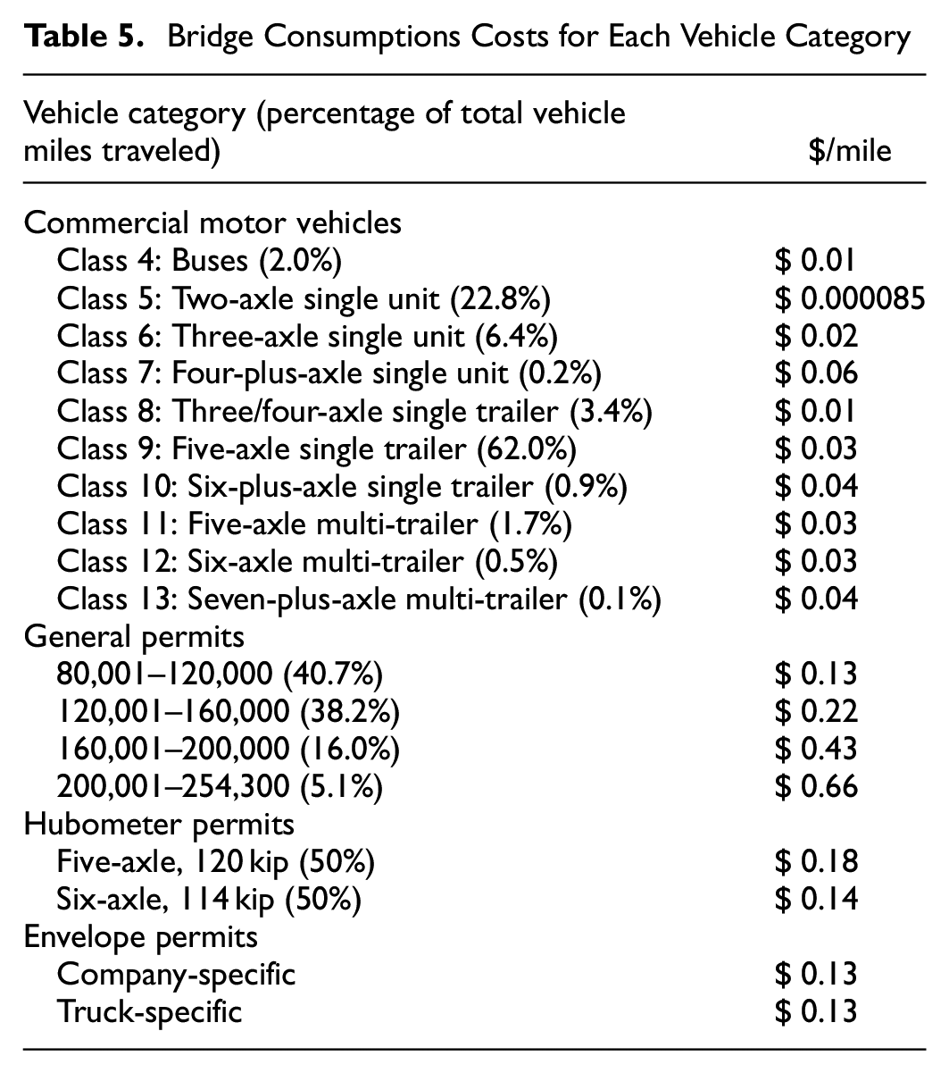
The highest bridge consumption cost per mile was found to be the OW vehicles on the General Permit, with a weighted average cost (based on VMT) of $ 0.24/mile, followed by Hubometer Permits with $ 0.16 and the Envelop Permits with $ 0.13/mile. Even though the lowest proportional cost per mile was found on Commercial Vehicles, with a weighted average of $ 0.022/mile, it is important to notice that this category was responsible for the majority of the statewide VMT, which resulted in 85.8% of the total bridge consumption cost. General, Hubometer, and Envelope Permits represented only 5.8%, 1.7%, and 6.7%, respectively.
Conclusion
The consumption cost analysis for bridges on Texas roads provides valuable insights into the funding needs and potential revenue sources for bridge maintenance and improvement. With the state of Texas maintaining the largest bridge inventory in the U.S., ensuring the safety and efficiency of these structures is of utmost importance for the economy and transportation system of the state. The study focused on assessing the bridge consumption costs for commercial vehicles and OS/OW vehicles.
The analysis considered factors such as VMT and bridge fatigue concepts to calculate the bridge consumption costs per mile. The study accounted for different traffic configurations and utilized data from the Central Permit Office to gather information on OW vehicles (e.g., axle weights and spacings) necessary to characterize them. The analysis findings highlighted the significant impact of OW vehicles on bridge consumption costs and the need of separate analysis for eastern and western counties of Texas, because of bridge density differences. The Monte Carlo simulation approach enabled the evaluation of approximately 20,000 annual miles of road segments and associated bridges, providing a comprehensive assessment of bridge consumption costs statewide, which leads to an average cost for each vehicle category.
The results of the analysis can serve as a basis for policy and decision-making about bridge maintenance funding and fee structures for OS/OW permits. Results indicates that the highest cost per mile for bridge infrastructure was attributed to General Permits carrying 120 to 253.3 kip. However, the heavily skewed VMT of commercial vehicles resulted in them being responsible for approximately 85.8% of the total bridge consumption, while OS/OW vehicles such as General, Hubometer, and Envelope permits accounted for the remainder.
Further research on funding methods and alternative revenue streams has the potential to significantly contribute to ensuring the safe and efficient transportation of people and goods across the state’s infrastructure. The comprehensive framework and understanding of bridge consumption costs shown in this study can aid the state of Texas in taking proactive measures to maintain a satisfactory level of serviceability for its road and bridge network while supporting economic growth and development.
Footnotes
Author Contributions
The authors confirm contribution to the paper as follows: study conception and design: J. Weissmann, A. Weissmann, J. Prozzi; data collection: J. Weissmann, A. Weissmann, J. Prozzi; analysis and interpretation of results: J. Weissmann, D. Inoue, A. Weissmann, J. Prozzi; draft manuscript preparation: J. Weissmann, D. Inoue. All authors reviewed the results and approved the final version of the manuscript.
Declaration of Conflicting Interests
The author(s) declared no potential conflicts of interest with respect to the research, authorship, and/or publication of this article.
Funding
The author(s) disclosed receipt of the following financial support for the research, authorship, and/or publication of this article: This work was supported by an Interagency Contract with the Texas Department of Transportation.