Sage Journals: Discover world-class research

Abstract

Traffic management in work zones is a challenging task that requires a balance between creating a safe environment for workers and minimizing traffic delays. Accurately predicting travel times through work zones is essential for dynamic traffic management and reducing congestion. However, complex interrupted traffic patterns in work zones (also known as construction zones) make this challenging compared with regular traffic congestion and free-flow conditions. To address this complexity, the paper develops a data-driven deep feed-forward artificial neural network to forecast under-construction travel times in work zones using an integrated data set of almost half a million observations. The variables considered in the neural network include the work zone characteristics, road design features, weather information, and traffic flow information. The raw data set comprised approximately 15 million travel time observations collected at 674 work zones. After cleaning and preprocessing the data and applying feature engineering techniques, the raw data set was reduced to 81 work zones spread along a 700 km corridor between the western borders of Alberta and Vancouver, British Columbia. The data were split into training and test data using a 90:10 ratio. Training data were used to develop a 27-input neural network with four hidden layers. After validating the test data, the neural network achieved a root mean squared error of 0.150 min and an R-squared score of 0.945, indicating a high accuracy level in estimating the under-construction travel time.

Keywords

work zone delay time under construction travel time estimation artificial neural network non-recurrent traffic congestion data driven modeling operations interrupted flow travel time traffic flow theory and characteristics traffic flow

The highway network is intended to facilitate the safe and efficient movement of people and goods and plays a vital role in the economic growth of nations. An interconnected and safe road network reduces travel time and cost. Thus, highway traffic congestion should be effectively monitored and managed to minimize delays and reduce greenhouse gas emissions while maintaining a safe driving environment.

Traffic congestion can be classified as recurrent congestion, which occurs during peak hours, and nonrecurrent congestion, which occurs as a result of accidents, spills, and debris on roadways, inclement weather, or the existence of work zones (WZs) ( 1 – 3 ). WZs or construction areas are laid out at locations where maintenance or construction activities such as paving, marking, patching, surfacing, or utility works occur. According to the United States Department of Transportation Federal Highway Administration’s (FHWA) report ( 4 ), WZs account for 24% of nonrecurrent traffic congestion. Such WZs are estimated to result in 60 million vehicles per hours of capacity loss because of closed lanes, narrow roads, and slow speeds. This challenge in predicting travel times through WZs and delays because of them is a result of the complex, interrupted, stop-and-go traffic patterns such areas introduce. To manage traffic flow appropriately, especially during traffic peaks, simply increasing speed through WZ areas is not an appropriate solution, because it exposes construction workers to high safety risks. Instead, an accurate estimate of anticipated delays considering all different variables helps manage traffic situations and devise proactive strategies.

Probe vehicle data (e.g., Google and Waze) have been an extremely valuable source of travel time information and have been used in many projects to monitor travel times and delays ( 5 – 9 ), including the Trans Mountain pipeline construction project, which extends along the highway between western Alberta and Vancouver in British Columbia (BC). To ensure that delays caused by construction activities do not exceed the thresholds set by the BC Ministry of Transportation and Infrastructure (BCMoTI), the project team utilized probe vehicle data for real-time estimation of under-construction travel times. The difference between the under-construction travel time and travel time under normal conditions was then used to estimate the delay. Although such estimates were verified to be reliable in most cases, this was not the case in regions where cellular and global positioning system (GPS) coverage is poor because of under-construction travel time estimates being heavily reliant on historical data. This is common when construction activity takes place at remote locations and on long highway corridors, particularly in countries with a large geographic footprint where areas of poor cell coverage are common.

Despite their importance, the majority of existing research on predicting and modeling delays in WZs has been limited to parametric and simulation studies. Recently, a few studies have attempted to forecast mobility in WZs using machine learning (ML) techniques. In fact, the lack of travel time prediction models for WZs has led most transportation agencies across North America to use simulation tools that have been developed to model freeway travel times, predict WZ impacts, and select optimal design and deployment strategies ( 10 ).

To address these gaps, we developed the first artificial neural network (ANN) ( 11 – 13 ) for predicting under-construction travel time (and delay) in WZs on a microscopic level using integrated environmental, WZ, traffic, temporal, and weather data. An essential advancement is including detailed weather factors, such as temperature, precipitation, and wind speed, as predictors, which previous WZ delay models have not accounted for. Furthermore, the model enables delay assessment on a microscopic level, at which variation in delay is analyzed on the same day, on different days during a week, and on different days during a month. The deep feed-forward neural network (FFNN) uses an extensive data set of about half a million records collected at 81 WZs. By harnessing real-time data collected across numerous WZs and conditions, the model provides new insights into the impact of environmental factors on delays and enables more effective dynamic traffic management. The model was also developed using data collected along a single corridor, which minimizes the impact of traffic-related confounding factors and results in the model focusing entirely on the effects of other characteristics. The combination of an extensive data set and microscopic analysis signifies the multifaceted contribution of our work, which, overall, enhances the comprehensiveness and precision of WZ delay prediction. It should be noted that ANNs are a modeling technique, and they were chosen for two reasons: (a) they make no assumptions about the underlying data; and (b) the large size of the data set and number of features make ANNs well suited to training such a complex model.

Literature Review

Studies on WZ Delay Prediction

Because collecting and aggregating comprehensive data from multiple sources is challenging, previous studies have been limited to the variables considered. For example, Du et al. ( 11 ) used a multilayer feed-forward neural network called multilayer perceptron (MLP) to estimate the WZ delay using probe vehicle data. They used data from different freeways in New Jersey in 2014 and considered segment speed, WZ length, ratio of open lanes, and basic WZ hours in their models. However, they did not account for detailed WZ characteristics such as transition lengths, lane closure details, traffic control elements, or environmental factors such as weather conditions. The results showed that the ANN model estimated travel delays more accurately than the traditional deterministic queuing model. In a later study ( 12 ), Du et al. integrated the previous ANN model with a support vector machine (SVM) to account for capacity in their predictions. In the hybrid model, the SVM layer predicts the WZ capacity, and this output is fed into the ANN, which regressed the 15-min speed data to predict spatiotemporal delays. The proposed hybrid model outperformed an ANN model that did not utilize traffic volume as a feature, thereby indicating that this was a crucial factor. The model’s performance was evaluated along three WZs, all only short segments of highway, and observations were collected over a short timeframe.

Using a connected vehicle environment, Wen ( 13 ) attempted to simulate WZ travel time. A simulation model was developed using data from a single WZ in New York. Travel time analyses were conducted using four types of models: linear regression; multivariate adaptive regression splines; stepwise regression; and elastic nets. Bae et al. ( 14 ) proposed a multicontextual approach for modeling the impact of urban highway construction WZs on traffic. They also utilized ML techniques to predict long-term traffic flow rates and the respective truck percentages. A third-order polynomial curve-fitting model was used to estimate WZ travel time delays in large urban cores.

To determine the impact of WZs on nonrecurrent delay separately, Chung ( 15 ) and Chung et al. ( 16 ) used one year (2009) of archive data from South Korea’s freeways. The model used a data set of 14 major freeways in South Korea. The results showed that the number of closed lanes, average daily delay, WZ length, and WZ duration directly affected the delay caused by the WZs. In another study, Morshedzadeh et al. ( 17 ) used ordinal logistic regression to assess the impact of spatial, temporal, environmental, and segment factors on delay. Key findings were that higher traffic volumes, peak hours, weekend travel, longer WZ length, and summer were associated with greater delays, whereas precipitation reduced delays.

Although some previous studies have focused specifically on predicting delays caused by WZs, this remains an emerging area of research with limited existing literature, as summarized in Table 1, which presents the key details and limitations of five existing models for estimating WZ delays. To provide additional context, the literature review was expanded to encompass studies that modeled and predicted other related WZ attributes as well as just delay time.

Table 1.

Summary of Existing WZ Delay Prediction Models

Study (reference)	Methodology	Data and sample size	Key details and limitations
Du et al. (11)	Multilayer feed-forward neural network	Number of observations not mentioned in the study	Considered segment speed, WZ length, open lane ratio, work hours; did not account for detailed WZ or weather factors; limited variables
Du et al. (12)	Hybrid ANN and SVM	181 WZs and 50,000 15-min speed records collected over a one-year period (2014)	Added WZ capacity prediction from SVM; limited WZ segments and timeframe; small sample size with limited variables
Wen (13)	Simulation model: linear regression; MARS; stepwise regression; elastic nets	34,560 observations from a single 2-mi New York State WZ	Simulated WZ travel time; compared multiple models; single WZ limits generalizability; did not account for factors outside the WZ that could have an impact
Bae et al. (14)	ANN for long-term predictions; third-order polynomial curve fitting for delays	17,518 traffic sensor readings; data for urban highway WZs in Los Angeles, CA	Predicted long-term traffic and truck percentages; estimated delays; did not focus on detailed microscopic delay prediction
Chung ( 15 ) and Chung et al. (16)	Statistical model	31,128 WZs over one year (2009) from 14 freeways in South Korea	Analyzed impact of WZ characteristics on nonrecurrent delays; older, limited data set from single country

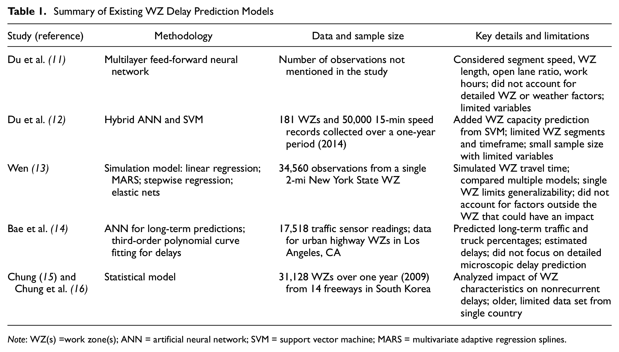
Note: WZ(s) =work zone(s); ANN = artificial neural network; SVM = support vector machine; MARS = multivariate adaptive regression splines.

Studies on Other WZ Attributes

Kamyab et al. ( 18 ) focused on capturing patterns in nonrecurrent traffic congestion, mainly when hourly traffic volume data were unavailable. To do so, the authors utilized historical lane closure information on Michigan Interstate highways between 2014 and 2017 to forecast the spatiotemporal mobility for future lane closures. Using probe vehicle data, a mobility profile for historical observations was created. This profile was used to train the random forest, XGBoost, and ANN models, among which the ANN outperformed the rest in accuracy. One drawback of this study is that it placed speed data into wide 20 mph bins, which makes a significant difference when the focus is on predicting delay on a microscopic level. Hou et al. ( 19 ) developed four models, namely, random forest, regression tree, MLP, and nearest neighbor nonparametric regression, to investigate both long- and short-term traffic flow forecasting. Using WZ data on two different types of roads, a freeway (I-270) and a signalized arterial (MO-141) in St. Louis, Missouri, U.S.A. The results showed that the random forest model achieved the most accurate traffic flow forecast.

Bian and Ozbay ( 20 ) also attempted the prediction of WZ capacity using data for WZs on freeways in seven U.S. states to develop two models: black box variational inference (BBVI) in the Bayesian neural network (BNN); and Monte Carlo (MC) dropout in regular ANN. In addition, the BBVI and MC dropout methods were compared with traditional methods such as ridge linear models and deterministic ANN. The results showed that although BBVI outperformed ridge linear regression and deterministic ANN, MC dropout yielded less accurate but acceptable results compared with BBVI. In a similar study, Weng et al. ( 21 ) developed a model incorporating uncertainty for estimating the WZ capacity. Their model is based on a mixed linear regression function, in which capacity is considered a random variable following a lognormal distribution. The parameters of this distribution were determined using the Bayesian approach. It should be noted that because of limitations in the available data, the study did not investigate the impact of additional factors, such as the existence of ramps and traffic control devices.

Lu et al. ( 22 ) investigated the effects of WZs on traffic speed–volume–density curves and the roadway capacity using traffic data collected on freeways in Iowa, U.S.A. Four WZs in Iowa were investigated in this study during the 2015 and 2016 construction seasons. A modified five-parameter logistic model was developed to describe the speed–density relationship, based on which an operational capacity prediction method was proposed considering the relationship between free-flow speed and WZ characteristics. The results showed that the logistic model-based method can predict a speed–density relationship that is close to the estimated one from field data. Moreover, the predicted operational capacities based on the proposed method were closer to the estimated values than those proposed by the decision tree-based approach developed by Weng and Meng ( 23 ).

Before these studies were undertaken, classical ML methods were also developed. Weng and Meng ( 23 ) developed a decision tree-based model to estimate freeway WZ capacity accurately. F-test splitting was used as a criterion to split the nodes and further grow the tree. Pruning was applied to minimize the mean square error (MSE) of the predictions. Subsequently, another study ( 24 ) used an ensemble tree approach to estimate the WZ capacity. The ensemble tree model prediction was more accurate than that of the model based on a single decision tree.

In collaboration with the Center for Transportation Research in Austin, Texas, the Smart Work Zone Deployment Initiative published a report summarizing efforts to develop ML models for predicting the impact of WZs on traffic, including local speed and traffic volume changes and corridor-level travel time increases ( 25 ). The researchers implemented ANNs to forecast speed and volume changes for planned closures. The researchers also analyzed the performance of three short-term travel time prediction techniques: a time-series analysis model; and two types of ANNs. The study found that on average, the new models outperformed traditional approaches by up to 50% during the peak period travel time prediction; however, the study noted that the performance was not as reliable for predicting travel times when WZs were present. It concluded that the results were promising, with ML models consistently outperforming traditional approaches.

In addition to recent ML techniques, traditional analytical and simulation models have been widely used for WZ impact assessments. The Highway Capacity Manual (HCM) proposed methods for estimating the WZ capacity based on lane closures and speed reductions ( 26 ). However, HCM methods rely on generalized parameters that may not capture site-specific conditions. Microscopic traffic simulation tools, such as PTV Vissim ( 27 ) and TSIS-CORSIM ( 28 – 30 ), model the movement of individual vehicles through WZs under different scenarios. However, simulations require detailed coding of network geometry, traffic control, driver behavior models, and calibration to local conditions. Critical lane volume techniques, such as Highway Capacity Software, analyze the intersection level of service and delays at signalized intersections affected by WZs. Analytical queuing methods, such as the Queue and User Cost Evaluation of Work Zones ( 31 ), can estimate expected queue lengths and delays based on WZ capacity reduction. However, queuing methods require accurate inputs for arrival rates and capacity. These traditional analytical and simulation modeling approaches have been valuable for WZ assessment. However, they rely on traffic flow and driver behavior approximations, which may not fully reflect real-world intricacies. By contrast, data-driven ML offers new opportunities for modeling delays based directly on field observations of travel times through WZs under various conditions.

Further studies have attempted to model and predict other WZ features such as capacity (32, 33), speed (22, 34), queue length ( 35 – 37 ), and safety ( 38 – 42 ). Meng and Weng’s ( 43 ) heterogeneous cellular automata model of traffic delay in WZs demonstrated that particularly in light traffic conditions, the length of the transition area has far more significant effects on traffic delay than the length of the activity area.

As summarized in Table 1, only a limited number of previous studies have directly focused on modeling delays caused by WZs. More common were studies that used both classical and ML tech to predict the impact of related features such as WZ capacity, speed, and queue length. In particular, few existing works leverage ANNs for WZ delay estimation, and those that do rely on relatively small data sets collected over short time periods. This makes it difficult to develop robust, generalizable models. Moreover, most previous research uses estimated rather than observed WZ capacity data. A critical gap is that external factors such as weather and temporal variables are often excluded.

To address these limitations, this study develops an ANN model for predicting WZ delays. The model is trained on a large data set of half a million observations collected along a 700 km highway corridor over two years. This extensive sample captures variance across seasons, times, and locations. Additionally, the capacity information is observed, as opposed to that used to develop the travel time prediction models in previous work, which was estimated. Detailed weather data enriches the model, alongside temporal variables and multiple WZ characteristics. The robust methodology and comprehensive data set are an advance on previous work and aim to deliver enhanced predictive accuracy. This study also provides new insights into the impact of WZ attributes, traffic conditions, time, weather, and other factors on delay.

Data Collection and Description

The data used in this study were collected by the IntelliTrafik division of ATS Traffic, a traffic technology company headquartered in Edmonton, AB. The raw data included approximately 15 million travel time observations, captured every 2 to 3 min and collected between 2021 and 2022 along the 700 km corridor between the western borders of Alberta and the City of Vancouver in BC, Canada. The corridor includes 710 planned WZs as part of the Trans Mountain expansion project. Of these, 674 were already activated during the period the travel time data were being collected. We focused on the year 2022 because of the impact of COVID-19 on traffic patterns and WZ activities in 2021. Along with travel time data, the specification design details of 123 WZs on Highway 5, where the posted speed limit is 100 km/h, were extracted directly from WZ plans. The remainder of this section provides details on the variables used in our ANN model to predict under-construction travel time.

Dependent Variable—Under-Construction Travel Time

Travel time data used in this study were collected from Google’s probe vehicle data every 2 to 3 min for each active WZ. Google data are available from a service provider in a readily usable format. In addition, travel time sensors that use Bluetooth and Wi-Fi signals were installed at a selection of road segments to validate travel time estimates using field ground truth data.

Weather Variables

One-hour weather data records were gathered from 40 Environment Canada weather stations in BC and appended to travel time information. These data are maintained by the Government of Canada’s environment resources ( 44 ). Weather data include hourly Temperature, Precipitation, and Wind Speed information. This information was linked to the travel time observations based on temporal and location data. An automated script was written to perform the execution of the data collection procedure.

Temporal Variables

Because traffic volume and congestion typically differ between different days and different seasons, certain variables were defined. For example, the Season variable represented the season during which data were collected; construction activity is often limited to summer and spring, and only two seasons existed in the data set. Other extracted variables were Minute in Day, Hour, Weekday (0 for Monday to 6 for Sunday), Day in Month, Day of Year, and Month.

Segment-Related Variables

Road Type and Travel Direction

WZs are located along different corridor sections and include two road types: multilane undivided roadways; and two-lane, two-way roadways. Each road segment could be leading traffic in two directions. In a situation in which the traffic is moving away from Vancouver to the border of Alberta, the road segment is northbound. If the traffic is moving toward Vancouver, it is southbound.

Traffic Volume

Traffic volume information is also crucial when modeling travel time, and this was obtained through BCMoTI’s Traffic Data Program. As part of this program, BCMoTI installs multiple permanent and temporary traffic counter sites at various locations throughout British Columbia ( 45 ). A script was written to locate traffic count sites near to each WZ automatically.

It is worth noting here that some of the traffic counter sites were permanent, whereas others were temporary. For temporary traffic count stations, traffic volumes during the times when travel time data were collected were not always available. To account for this, the hourly traffic volume (HTV) information for those records was estimated using the following projection equation recommended in the Alberta Highway Geometric Design Guide ( 46 ) for annual average daily traffic projections (Equation 1).

HTV' = HTV \times (1 + (TGR \times (CY - RY)))

(1)

where $HTV' =$ estimated $HTV$ during the current year $(CY)$ ,

$HTV =$ observed $HTV$ during the most recent year for which data are available $(RY)$ ,

$TGR =$ traffic growth rate (assumed to be 1%),

$CY =$ current year, and

$RY =$ recent year—the most recent and latest year for which data are available.

Segment Length

As well as traffic volume, segment length was also considered in the models. This is defined as the distance between two points that represent the start and end points of the traffic control area for a construction site as outlined in the approved traffic control plan.

WZ Characteristic Variables

The WZ characteristic variables provide information about the specific features of the construction WZs. These variables together help enhance predictions for under-construction travel time, and a description of them is given in Table 2. Additionally, Figure 1 provides a depiction of these variables on a WZ layout.

Table 2.

WZ Characteristic Variables Definition

Variable	Description
Construction sign speed limit distance	Distance between the “Construction Ahead” sign and the first speed limit sign
1st transition length start	Distance between the first speed limit sign before the WZ and the WZ speed limit sign
2nd transition length start	Distance between the WZ speed limit sign and the “Traffic Control Person” sign
Transition speed limit	Speed limit before entering the WZ
Prepare to stop?	Presence of a “Prepare to Stop” sign just before the WZ area
WZ length	Total length of the WZ (distance between “Traffic Control Person” signs at both ends)
WZ speed limit	Designated speed limit within the WZ
Barrel spacing	Spacing between traffic control barrels within the WZ area
Minor approach?	The presence of an intersection or side road within the WZ area
Transition length end	Distance between the end of the WZ and the “Thank You” sign or the first speed limit sign after exiting the WZ
Thank you sign speed limit distance	Distance between the “Thank You” sign and the speed limit sign after exiting the WZ
Bidirectional WZ?	Indicates if the WZ allows traffic flow in both directions (0 for separate lanes, 1 for shared lane)
Originally divided?	Indicates if the original lane configuration had a divider between the two bounds
Original lane count	Number of lanes available to traffic before the WZ (1 or 2)
New lane count	Number of new lanes available within the WZ (usually 1)
Closed lane count	Number of lanes closed because of the WZ (0 or 1)

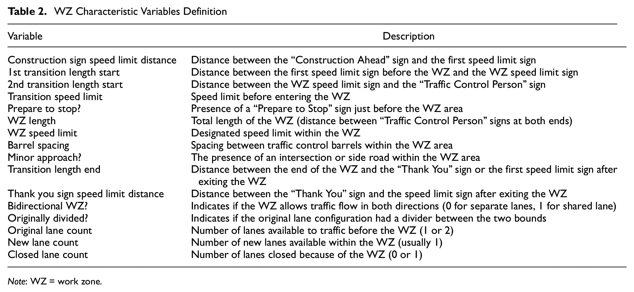
Note: WZ = work zone.

Figure 1.

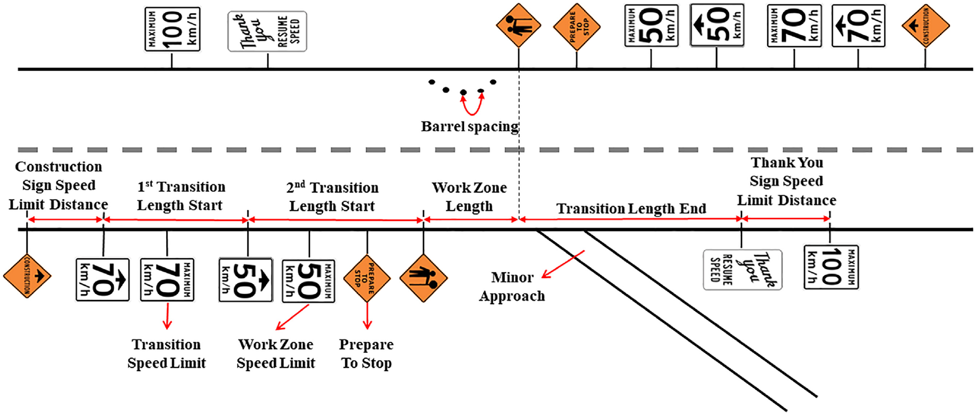
Features in a WZ plan.

With regard to the traffic control setup, which indicates the type of traffic control that is proposed for any work site, these WZs used single lane alternating traffic.

Data Set Summary

Once the data had been extracted, exploratory data analysis was performed, and data cleaning, integration, transformation, augmentation, reduction, refining, and sampling were undertaken. In addition, overall feature selection was carried out and engineering techniques were applied. Subsequently, these processes were merged, leading to 485,783 records for 81 activated WZs. The box plot and descriptive statistics of numerical variables are summarized in Figure 2 and Table 3, respectively. The transition speed limit through the WZs is 70 km/h. Table 4 shows the frequency and respective proportions of categorical variables.

Figure 2.

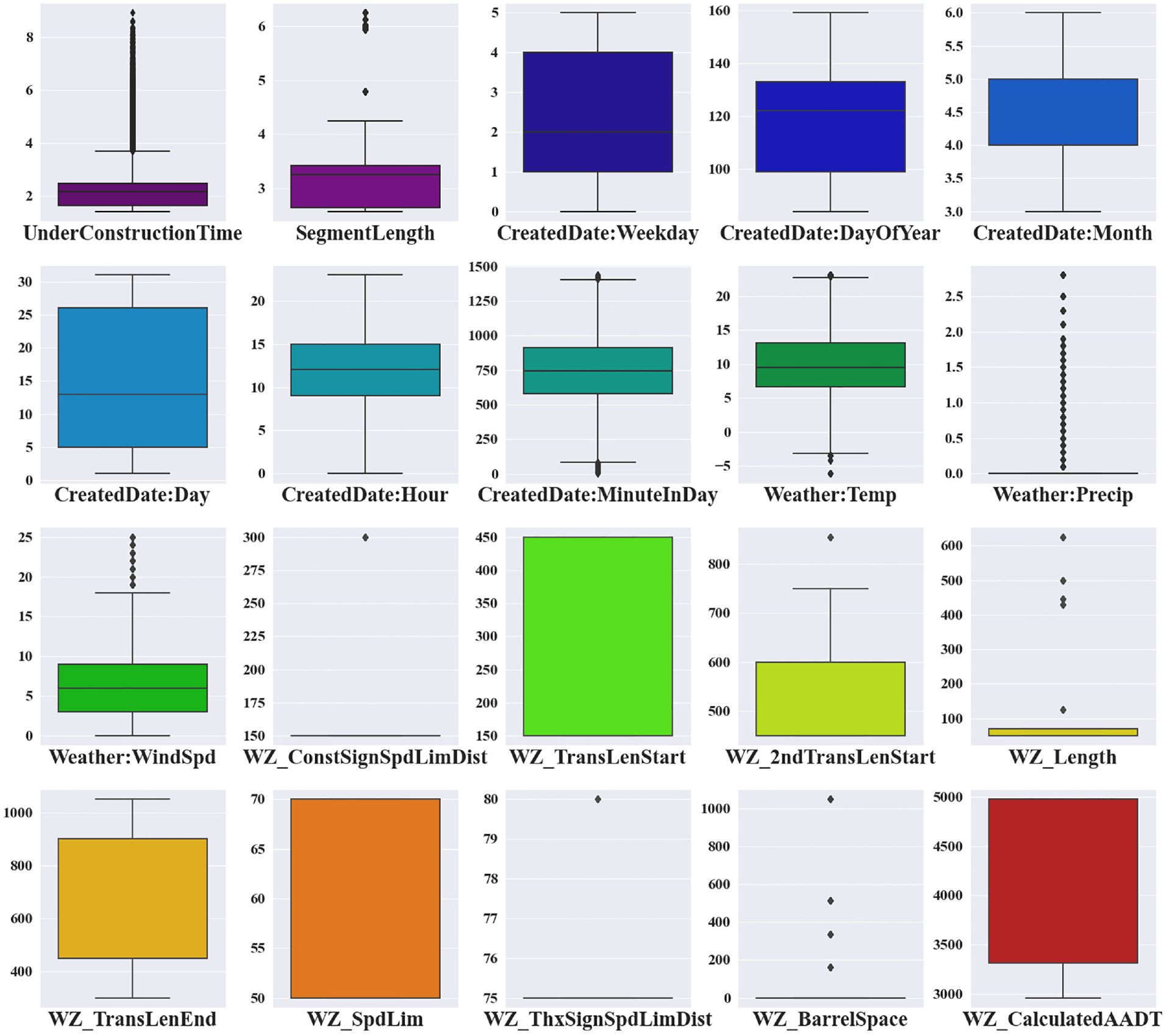
Box plot for numerical variables.

Table 3.

Descriptive Statistics of Numerical Variables

	Mean	SD	Min.	25%	50%	75%	Max.
Under-construction time (minute)	2.17246	0.65666	1.4	1.62	2.15	2.45	8.93
Segment length (km)	3.23367	0.75538	2.567	2.642	3.248	3.42	6.25
Weekday	2.2372	1.62964	0	1	2	4	5
Day of year	120.2022	20.83762	84	99	122	133	159
Month	4.49565	0.81174	3	4	5	5	6
Day	15.3634	10.56314	1	5	13	26	31
Hour	11.91606	3.22515	0	9	12	15	23
Minute in day	744.7889	193.1409	2	580	742	911	1438
Temperature (°C)	9.80764	4.90612	-6.1	6.6	9.5	13.1	23.1
Precipitation (mm)	0.07866	0.29483	0	0	0	0	2.8
Wind speed (km/h)	6.738	4.71748	0	3	6	9	25
Traffic volume (vpd)	3916.956	830.5267	2958.16	3308.55	3308.55	4976.96	4976.96
WZ transition length start	287.2736	149.4593	150	150	150	450	450
WZ 2nd transition length start	500.1309	83.52551	450	450	450	600	855
WZ length	146.8693	173.9146	50	50	70	70	625
WZ transition length end	636.6251	204.6725	300	450	450	900	1050
WZ construction sign speed limit	172.8244	53.87682	150	150	150	150	300
WZ thank you sign speed limit	75.00339	0.13008	75	75	75	75	80
WZ barrel spacing	104.7710	234.6021	0	0	0	0	1050
WZ speed limit	60.84842	9.96395	50	50	70	70	70

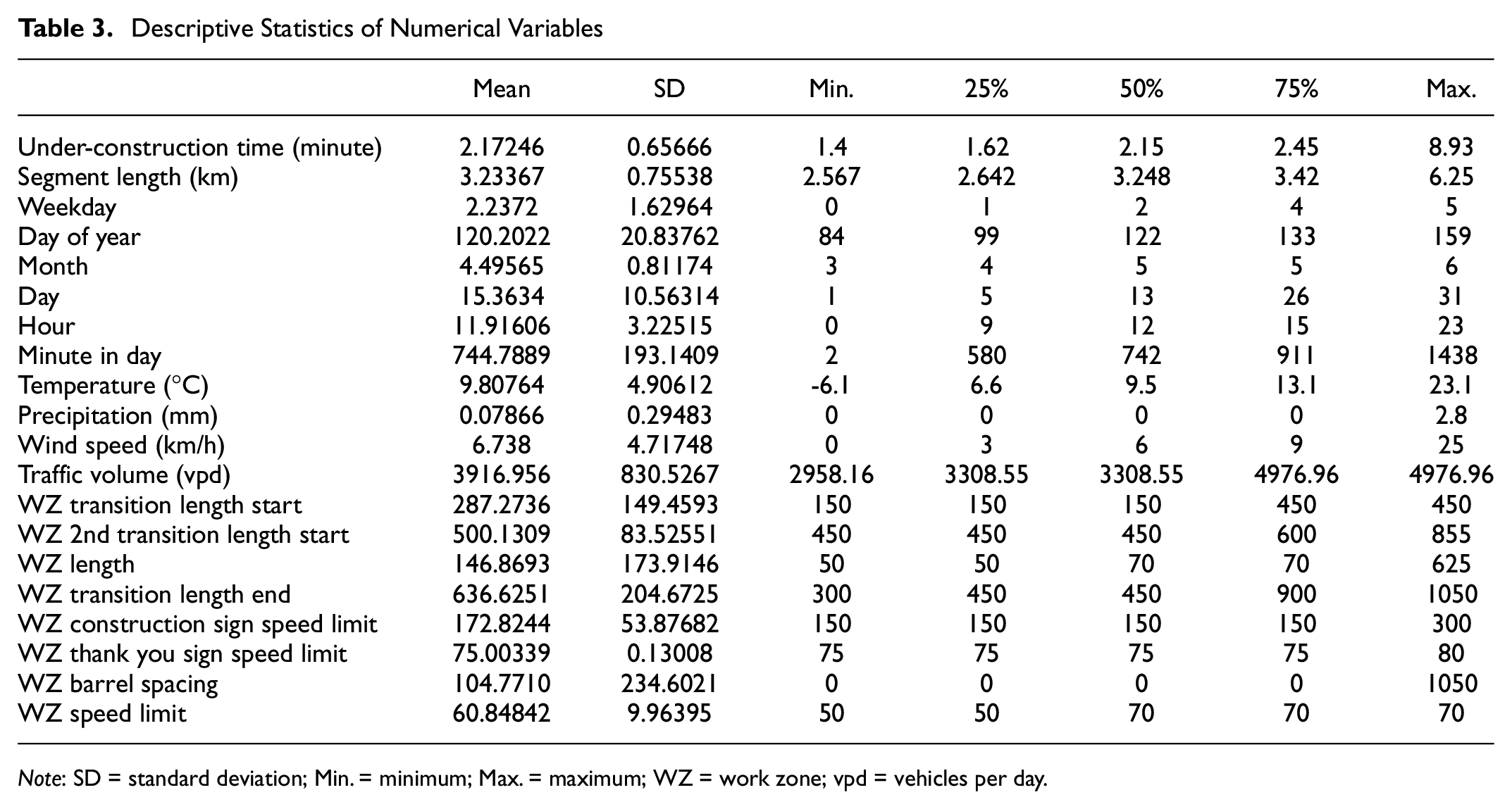
Note: SD = standard deviation; Min. = minimum; Max. = maximum; WZ = work zone; vpd = vehicles per day.

Table 4.

Summary of Categorical Variables

Categories	Frequency
Travel direction
Northbound	245,425 (50.5%)
Southbound	240,358 (49.5%)
Road type
Two-lane, two-way roadway	266,632 (54.9%)
Multilane undivided roadway	219,151 (45.1%)
Season
Spring	443,589 (91.3%)
Summer	42,194 (8.7%)
Bidirectional WZ?
No, not shared	358,334 (73.8%)
Yes, shared	127,449 (26.2%)
Were lanes originally divided?
No, no divider	385,100 (79.3%)
Yes, divider exists	100,683 (20.7%)
Number of lanes before WZ
1	478,501 (98.5%)
2	7,282 (1.5%)
Number of closed lanes
0	367,022 (75.6%)
1	118,761 (24.4%)
Minor approach exists?
No	313,387 (64.5%)
Yes	172,396 (35.5%)

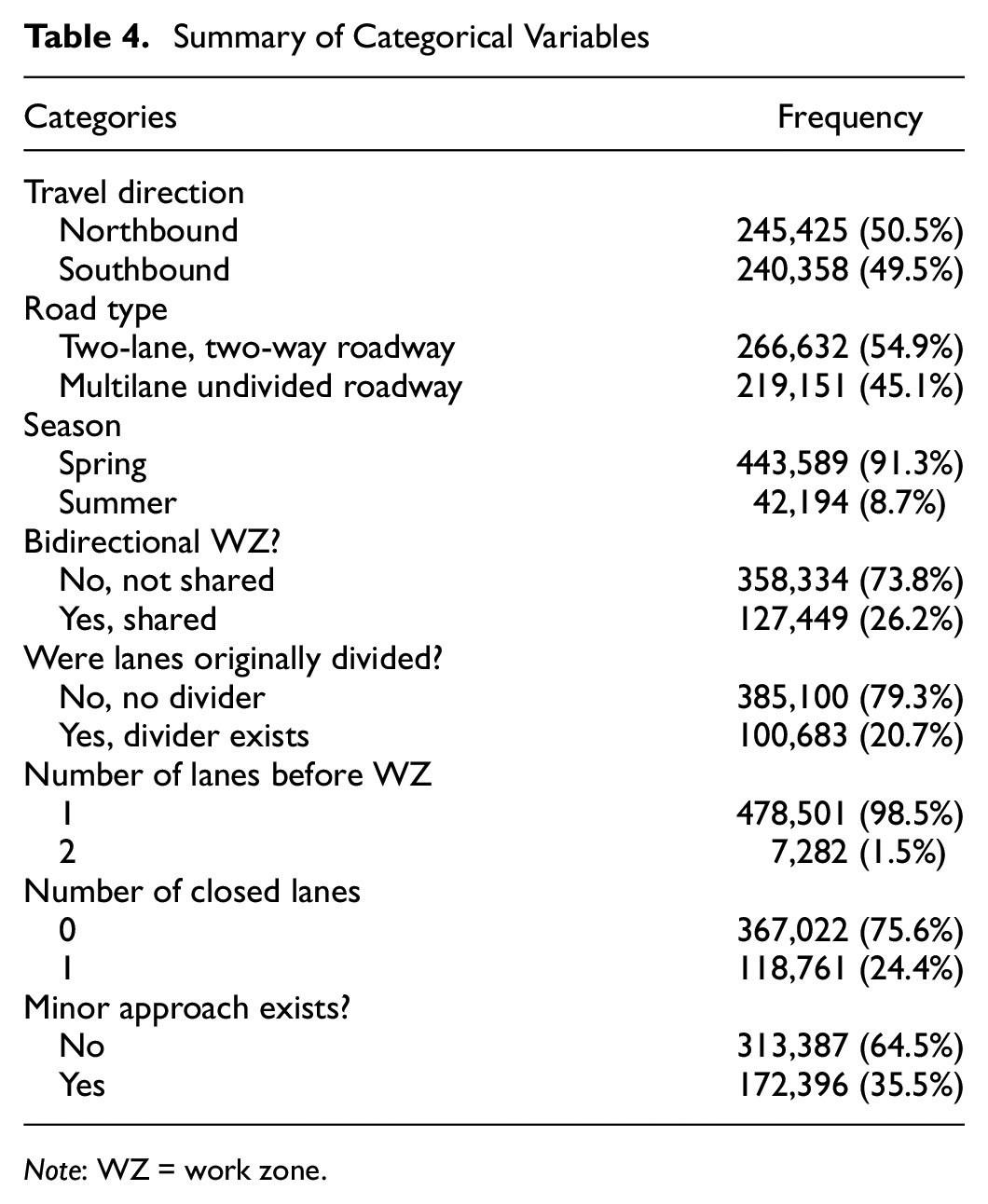
Note: WZ = work zone.

Data Preprocessing

As mentioned, the data set contains categorical, cyclical, and numerical features. Overall, these encoding techniques transform the raw data set into a numerical representation suitable for training ML models.

To handle categorical data, one-hot encoding, which converts categories into binary indicators, is applied. This allows categorical values to have a numerical representation. For cyclical features such as time, date, and so forth, which have periodicity, sinusoidal/cosinusoidal encoding is used. The periodic nature is captured by converting the cycles into corresponding sine and cosine components. Numerical features are normalized to a standard range using min–max scaling. This rescales the data to a common scale and cancels the impact of vastly different ranges of features.

To generate the split, the initial step was to shuffle the entire data set (485,783 records) in a random fashion to mix up the sample order. Once shuffled, the data set was split into training and test sets based on specified proportions. We used a 90:10 split, with 90% of samples (437,204 records) allocated to model training and validation and the remaining 10% kept exclusively for testing (48,579 records). Using a larger portion for training and validation provides more examples for the model to learn from, and shuffling ensures the test set is a random subset that reasonably represents the overall data distribution. In contrast to regression models, which frequently employ a conventional test/train split ratio, for ANN, there is no optimal divide that can be applied to all cases ( 47 – 51 ). According to the literature, what might be considered a low percentage, such as 10% of large data sets, can evaluate model performance adequately ( 52 , 53 ). The sizable test set obtained from a tiny portion of the huge data set still resulted in 48,579 test cases, which is significantly more than the number of samples usually used to develop and assess regression models. Thus, despite its seeming paradox, the 90:10 split maintains a large and representative test set and also enables strong neural network training. Thus, the enormous data set is put to good use in training and thoroughly evaluating unseen data.

Methodology

In this study, a deep fully connected FFNN was developed to predict travel time through WZs. The model takes in the preprocessed input features and passes them through multiple dense layers to learn nonlinear, complex relationships between the input features, for example, weather, traffic conditions, road attributes, and output travel time. The multiple layers and nonlinear activation functions provide the capacity for modeling real-world intricacies of WZ traffic flow.

ANN is a computational model based on the idea of how neurons in the human brain are connected. In ANNs, a neuron is a function of the summation of inputs, with the history from the past being a contributing factor to interconnection weights ( 54 ). McCulloch and Pitts further developed this idea into a computational model of neurons ( 55 ). In 1949, the Hebbian learning algorithm was proposed to adapt weights for learning examples ( 56 ). Rosenblatt then introduced perceptron, the first ANN that was influenced by visual perception in humans ( 57 ).

FFNNs are comprised of multiple layers of interconnected nodes or neurons. By using multiple computational units, called artificial neurons, the model is trained to capture the complex patterns and relationships within data sets. The learning and transfer of knowledge happens through the weighted connections between neurons in the hidden layers and output layer. More specifically, each neuron receives inputs from the previous layer, calculates a weighted sum (w₁, w₂, …, w_m) of its m inputs (x₁, x₂, …, x_m) to which a bias term b is added, applies an activation function f to produce the output y, and passes it to neurons in the next layer:

y = f ((\sum_{i = 1}^{m} w_{i} * x_{i}) + b)

(2)

This allows each neuron to learn a nonlinear combination of the inputs to approximate the target function, that is, the pattern of the output.

Model Training

The process of training an ANN is a fundamental aspect of its functionality. As mentioned earlier, the training process enables the ANN to make accurate predictions or classifications by adjusting its internal parameters, often referred to as weights and biases. Training an ANN typically involves the following key steps:

Initialization: Initially, the weights and biases of the network are assigned random values. These initial values serve as starting points for the training process.

Forward pass: During training, input data are processed through the network’s layers. Each neuron in the hidden layers produces an output (Equation 2). This output is then passed to neurons in the subsequent layer.

Error calculation: The network’s predictions, generated using the current weights, are compared with the actual target values. The difference between the predicted and true values (error) is calculated for each data point in the training data set (refer to the section titled Model Evaluation).

Backpropagation: The backpropagation algorithm is employed to propagate these errors backward through the network. It computes how much each weight contributed to the overall error. The weights are then updated in a way that minimizes this error, often through optimization algorithms based on gradient descent.

Steps 2 to 4 are repeated for multiple epochs. During each epoch, the weights are fine-tuned according to the errors encountered in the forward pass. The process continues until the model converges, meaning that the errors are minimized and the model’s predictions closely match the actual data. This training process results in a set of optimized weights and biases that enable the ANN to make accurate predictions or classifications. These optimized parameters represent the network’s learned knowledge of how the input data relate to the desired output. The trained ANN is then ready to make predictions or classifications based on new unseen data.

Model Development

The network consists of an input layer to receive the encoded 27-feature vector, followed by four hidden layers of 128, 512, 256, and 128 neurons, respectively, as illustrated in Figure 3. Each hidden layer applies the rectified linear unit activation function ( 58 ) to learn nonlinear combinations of the inputs. Dropout regularization ( 59 ) with a rate of 0.5 is implemented on hidden layers to prevent overfitting. The parameters of the ANN, including the weights and biases, are learned through backpropagation ( 60 ), and the MSE between predictions and actual/observed outputs, also known as the loss (cost) function, is calculated. Subsequently, the adaptive moment estimation method ( 61 ) is used to update parameters to minimize the loss function. The output layer contains a single neuron with a linear activation function to predict the continuous target variable of travel time.

Figure 3.

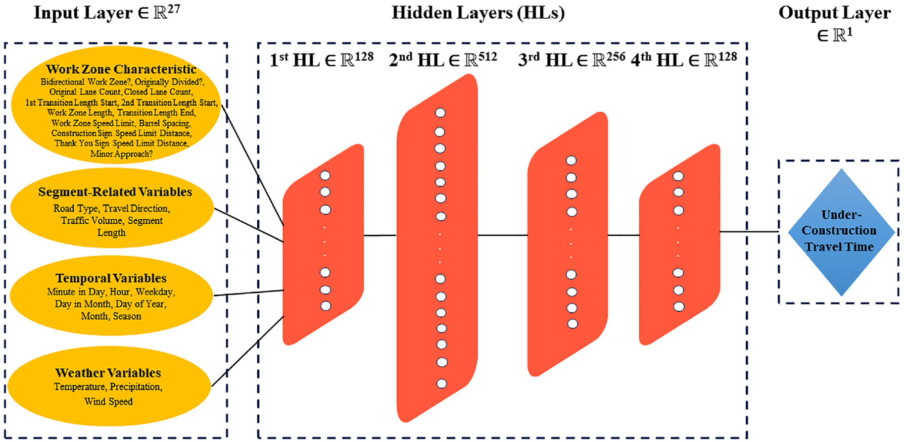
Architecture of ANN and input variables.

Model Evaluation

The performance of the deep ANN was evaluated using various regression metrics between the predicted and observed travel times. The model optimizes for MSE during training (loss function), thus measuring the average squared difference between the n pairs of predicted ( $y_{i}^{^}$ ) and actual values ( $y_{i})$ (Equation 3).

M S E = \frac{1}{n} {(\sum_{i = 1}^{n} y_{i} - y_{i}^{^})}^{2}

(3)

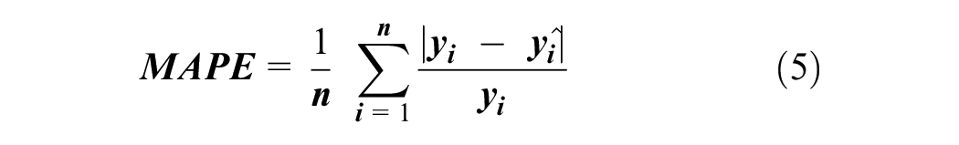
The more interpretable measure of MSE is root mean squared error (RMSE), which takes the square root of MSE and converts the unit of errors to minutes. RMSE is the standard deviation of prediction errors. Additional metrics include mean absolute error (MAE), which calculates the average magnitude of errors or absolute errors (Equation 4), and mean absolute percentage error (MAPE), which measures error as a percentage of the actual value (Equation 5). The lower values of MSE, RMSE, MAE, and MAPE imply higher accuracy of a regression model.

MAE = \frac{1}{n} \sum_{i = 1}^{n} | y_{i} - y_{i}^|

(4)

MAPE = \frac{1}{n} \sum_{i = 1}^{n} \frac{| y_{i} - y_{i}^|}{y_{i}}

(5)

The R-squared or R² score is the coefficient of determination and evaluates the goodness of fit. It indicates how well the input variables in the model can explain the variability in the output variable (Equation 6). R² normally ranges between 0 and 1 with the higher R² value having a better fit to observations.

R^{2} = 1 - \frac{\sum_{i = 1}^{n} {(y_{i} - y_{i}^)}^{2}}{\sum_{i = 1}^{n} {(y_{i} - \bar{y})}^{2}}

(6)

Results and Discussion

The model was trained using 437,204 samples and evaluated on 48,579 samples, with each input vector having a dimension of 27. The code is implemented using Python 3.11 in PyTorch 2.0.1 with CUDA 11.7. The model is trained for 800 epochs with a batch size of 1,024. Early stopping is used to prevent overfitting. Specifically, early stopping was used with validation loss as the monitored metric to track the performance of the model on a validation set after each training epoch. It used a mode of minimization and patience of 200 epochs. This allowed sufficient training iterations for the model to converge, but prevented excessive training. If the validation loss did not decrease for 200 consecutive epochs, training was automatically stopped. On an NVIDIA GeForce RTX 3090 GPU, model training took approximately 43 min. Once trained, the model can rapidly provide WZ delay predictions, with an average inference time of 150 ms per query.

Once trained, the model achieved an RMSE of 0.150 min in predicting under-construction travel time. The reported values are MSE = 0.023, MAE = 0.092, MAPE = 0.041, and R² score = 0.945, evaluated on the test set. Figure 4 plots model predictions (y-axis) versus actual (x-axis) under-construction travel times. The close alignment of the scattered plot to the diagonal line (x = y) indicates the model’s ability to estimate WZ travel times accurately considering input features.

Figure 4.

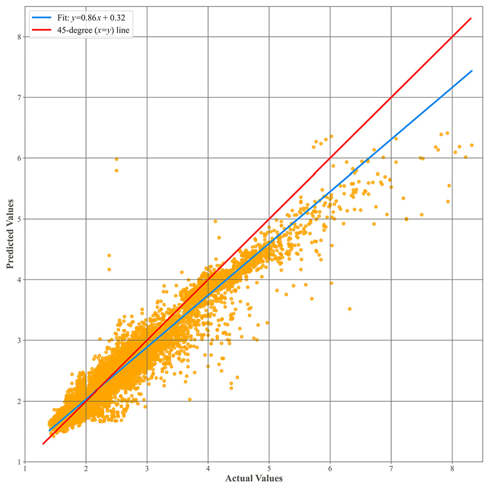
Actual versus predicted under-construction travel times (in minutes).

Indeed, as well as estimating the RMSE and R² variables, the model was explicitly evaluated according to scenarios that led to high under-construction time, resulting in predictions close to observed travel time. This is also confirmed and apparent in Figure 4. Increased deviations at higher travel times could be attributed to a relative lack of data points for very high travel times compared with moderate travel times. In cases in which there are fewer examples to train on, the model’s ability to predict outliers could be less certain.

In addition to the primary training approach, the impact of the k-fold cross-validation method ( 62 – 64 ) during training was also evaluated. The model underwent five-fold cross-validation, with each fold trained for 200 epochs using batches of 1,024 samples. Early stopping with a patience of 100 epochs was also applied in each fold. The model achieved an RMSE of 0.161 min, MSE of 0.026, MAE of 0.102, MAPE of 0.047, and R² of 0.940 on the test set. Figure 5 illustrates the model’s predictions versus actual under-construction travel times when trained using k-fold cross-validation. These metrics obtained with cross-validation further confirm the model’s robustness and its ability to generalize to new data.

Figure 5.

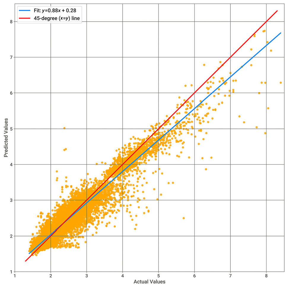
Actual versus predicted under-construction travel times (in minutes) using k-fold cross-validation.

The optimized values of model weights help analyze the importance of the input features (feature importance scores). Figure 6 compares each variable’s maximum effect on under-construction travel time (minutes). The maximum impact of a feature is measured as the difference between the maximum and minimum travel time predictions for all the variations of that feature. The bar plot visualizes the feature importance for the under-construction time (dependent variable), highlighting features with an impact greater than 0.4. Each bar represents a feature, and its length corresponds to its impact on the target variable.

Figure 6.

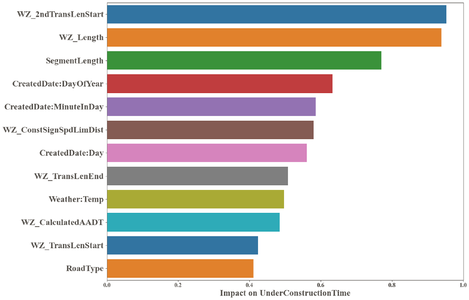
Feature importance for under-construction travel time.

According to Figure 6, WZ 2nd Transition Length Start, WZ Length, and Segment Length are identified as the top three most influential features with impact scores of 0.954, 0.939, and 0.771, respectively. Other features, such as Day of Year, Minute in Day, Construction Sign Speed Limit Distance, WZ Transition Length End, Temperature, and Traffic Volume, also exhibit significant impacts, with scores above 0.4. Conversely, some features, such as WZ Speed and Minor Approach, have relatively low impact scores, suggesting they may have less influence on the dependent variable.

Figure 7 illustrates the more in-depth impact of these features on the prediction for under-construction travel time. More specifically, the red line plot shows how the predicted travel time changes as the value of a single input feature is varied while keeping all other inputs constant at their median values. The overlaid histogram shows the distribution of that feature’s values in the actual data. This illustrates the sensitivity of the predictions to that particular feature; a steeper line or wider spread along the output (y) axis indicates that the feature has a more significant impact on predicted travel time.

Figure 7.

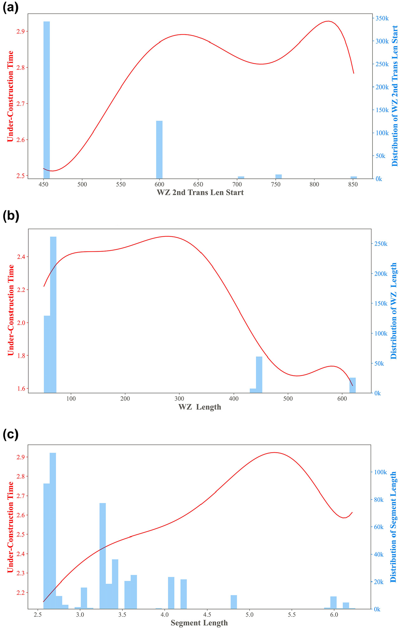
Impact of top three features on under-construction travel time: (a) impact of WZ 2nd Transition Length Start; (b) impact of WZ Length; (c) impact of Segment Length.

The observed impacts of the top features, shown in Figure 7, align with intuitive expectations. WZ 2nd Transition Length Start has a notable effect, with travel time increasing from 2.5 to 2.9 min as this length rises from 450 to 650 m. This aligns with expectations, because more extended transition zones lead to speed reductions, contributing to delays. However, interestingly, the effect levels off for transition lengths above 650m. WZ Length also strongly influences predicted travel times, with delays increasing from 1.6 to 2.4 min as length goes from 0 to 300 m. Finally, unsurprisingly, Segment Length shows a steady travel time increase from 2.2 to 2.9 min as length grows from 2.5 to ∼5.2 km. Longer highway segments inherently require more time to traverse. The consistent upward slope indicates segment length has a proportional impact on travel time predictions.

The results reveal complex interactions, such as potential thresholds at which impacts taper off after initial increases. These data-driven insights can inform operational strategies to mitigate delays. Analysis of additional features revealed further intuitive relationships. The model predicts an increased travel time from 10:00 a.m. to 6:00 p.m. versus early mornings and late nights. Northbound travel has slightly longer times compared with southbound travel, probably resulting from underlying differences in the traffic volume leaving and entering Vancouver. Adverse weather conditions, such as high winds above 15 km/h and precipitation over 0.5 ml, also show positive associations. These intuitive observations further validate the robustness of the developed ANN. This suggests the extra distance of tapered lane closures and mergers introduces noticeable delays.

Because deep ANNs learn directly from real-world observations, the model can capture complex relationships and subtle nuances that affect travel time through WZs. The integrated data set provides a rich set of details, including WZ characteristics, weather information, and segment-related and traffic conditions, which allow the modeling of real-world intricacies. Unlike simulation methods that rely on approximations and assumptions, the data-driven model can learn representations from a wide range of feature combinations. Additionally, building the model using data from a single corridor minimizes confounding factors. This method keeps the model focused specifically on modeling the impacts of WZs, thereby reducing the effect of unknown, unaccounted for, and unmeasured attributes.

Conclusions and Future Research

This paper presented a deep ANN for predicting travel times through highway WZs. The model was trained on an integrated data set of nearly half a million samples containing WZ layout details, road attributes, weather data, and traffic conditions. The model achieved high accuracy on the test set with an RMSE of 0.150 min, an R² score of 0.945, and strong MAE and MAPE metrics.

Both the integrated data set, which includes different attributes, and the deep learning approach enabled the learning of real-world intricacies affecting WZ traffic flow. This model is a robust, helpful tool for dynamically monitoring and managing the impact of WZs on the highway. By specifying the input features, the model can calculate delays and travel times in milliseconds; therefore, traffic managers can check different configurations and finally take proactive actions such as modifying lane closures or adjusting speed limits to minimize congestion. This will help improve safety and meet delay thresholds.

The flexibility of the ANN structure to model complex data relationships, combined with its data-driven distribution-free benefits, make this technique well suited to generating accurate predictions. Given the strong performance demonstrated, ANNs should be considered a viable modeling approach for forecasting travel times through WZs. That said, comparing multiple ML algorithms, such as random forests, support vector regression, XGBoost, and other neural network architectures with traditional simulation approaches, provides valuable insights into their relative strengths and weaknesses for predicting travel time and delays in different situations. This comprehensive analysis will clarify the tradeoffs between the accuracy, interpretability, and computational efficiency of different methods. Conducting rigorous comparative studies will provide a more complete understanding of state-of-the-art ML for predictive WZ modeling. Therefore, we strongly recommend that this be considered in future work.

The developed ANN is an invaluable tool for intelligent data-driven traffic management in construction areas. Although the model considers a good range of attributes in its predictions, expanding the data set could help cover more uncommon WZ configurations. Moreover, future research is planned by the authors to test the model at locations with poor GPS and cell coverage and assess its performance against field-collected data.

Footnotes

Acknowledgements

The authors thank Ahmed Khataan and Amit Dhavale at the University of British Columbia for their help in extracting work zone characteristics.

Author Contributions

The authors confirm contribution to the paper as follows: study conception and design: Y. Morshedzadeh, S. Gargoum, A. Gargoum; data collection: Y. Morshedzadeh; analysis and interpretation of results: Y. Morshedzadeh, S. Gargoum; draft manuscript preparation: Y. Morshedzadeh, S. Gargoum, A. Gargoum. All authors reviewed the results and approved the final version of the manuscript.

Declaration of Conflicting Interests

The author(s) declared no potential conflicts of interest with respect to the research, authorship, and/or publication of this article.

Funding

The author(s) disclosed receipt of the following financial support for the research, authorship, and/or publication of this article: This research was funded by the Mitacs Accelerate Program, Grant Number GR024705, ATS Traffic (IntelliTrafik), and the United Arab Emirates University’s CBE Program.

ORCID iDs

Yeganeh Morshedzadeh

Suliman Gargoum

Data Accessibility Statement

The data used during the study are owned by ATS Traffic (IntelliTrafik) and are proprietary or confidential in nature. The authors do not have permission to share the data.

The funders had no role in the design of the study, in the collection, analysis, or interpretation of data, in the writing of the manuscript, or in the decision to publish the results.

References

Lomax

T. J.

Quantifying Congestion. Final Report. NCHRP Report No. 398. Transportation Research Board of the National Academies, Washington, D.C., 1997.

Dowling Associates, Berkeley Transportation Systems and Systems Metric Group. Measuring Non-Recurrent Traffic Congestion. Final Report. California Department of Transportation, Sacramento, CA, 2003.

Skabardonis

Varaiya

Petty

K. F.

Measuring Recurrent and Nonrecurrent Traffic Congestion. Transportation Research Record: Journal of the Transportation Research Board, 2003. 1856: 118–124.

Lomax

Schrank

Eisele

Urban Mobility Report 2021 – Mobility Division. Texas A&M Transportation Institute, College Station, TX, 2019.

Brennan

T. M.

Remias

S. M.

Manili

Performance Measures to Characterize Corridor Travel Time Delay Based on Probe Vehicle Data. Transportation Research Record: Journal of the Transportation Research Board, 2015. 2526: 39–50.

Olszewski

Dybicz

Jamroz

Kustra

Romanowska

Assessing Highway Travel Time Reliability Using Probe Vehicle Data. Transportation Research Record: Journal of the Transportation Research Board, 2018. 2672: 118–130.

Jenelius

Koutsopoulos

H. N.

Travel Time Estimation for Urban Road Networks Using Low Frequency Probe Vehicle Data. Transportation Research Part B: Methodological, Vol. 53, 2013, pp. 64–81. https://doi.org/10.1016/j.trb.2013.03.008.

Yang

Guo

Road Probing: RSU Assisted Data Collection in Vehicular Networks. Proc., 5th International Conference on Wireless Communications, Networking and Mobile Computing (WiCOM), Beijing, China, 2009.

Advani

Thakkar

Shah

Arkatkar

Bhaskar

A Wi-Fi Sensor-Based Approach for Examining Travel Time Reliability Parameters under Mixed Traffic Conditions. Transportation in Developing Economies, Vol. 6, No. 1, 2019, pp. 1–9. https://doi.org/10.1007/s40890-019-0089-1.

10.

Berthaume

Jackson

Berg

O’Donnell

Melson

C. L.

Validating the Performance of the FHWA Work Zone Model Version 1.0: A Case Study along I-91 in Springfield, Massachusetts. Transportation Research Record: Journal of the Transportation Research Board, 2018. 2672: 46–56.

11.

Chien

Lee

Spasovic

Mouskos

Artificial Neural Network Model for Estimating Temporal and Spatial Freeway Work Zone Delay Using Probe-Vehicle Data. Transportation Research Record: Journal of the Transportation Research Board, 2016. 2573: 164–171.

12.

Chien

Lee

Spasovic

Predicting Freeway Work Zone Delays and Costs with a Hybrid Machine-Learning Model. Journal of Advanced Transportation, Vol. 2017, 2017, article e6937385. https://doi.org/10.1155/2017/6937385.

13.

Wen

A Work Zone Simulation Model for Travel Time Prediction in a Connected Vehicle Environment. https://arxiv.org/abs/1801.07579v1. Accessed June 21, 2023.

14.

Bae

Choi

J. H.

Multicontextual Machine-Learning Approach to Modeling Traffic Impact of Urban Highway Work Zones. Transportation Research Record: Journal of the Transportation Research Board, 2017. 2645: 184–194.

15.

Chung

Assessment of Non-Recurrent Traffic Congestion Caused by Freeway Work Zones and Its Statistical Analysis with Unobserved Heterogeneity. Transport Policy, Vol. 18, No. 4, 2011, pp. 587–594. https://doi.org/10.1016/j.tranpol.2011.02.003.

16.

Chung

Kim

Park

Quantifying Non-Recurrent Traffic Congestion Caused by Freeway Work Zones Using Archived Work Zone and ITS Traffic Data. Transportmetrica, Vol. 8, No. 4, 2012, pp. 307–320. https://doi.org/10.1080/18128602.2010.522609.

17.

Morshedzadeh

Gargoum

Microscopic Analysis of Work Zone Delay Using Big Data and Logistic Regression. Proc., Transportation Association of Canada, Ottawa, ON, 2023.

18.

Kamyab

Remias

Najmi

Rabinia

Waddell

J. M.

Machine Learning Approach to Forecast Work Zone Mobility Using Probe Vehicle Data. Transportation Research Record: Journal of the Transportation Research Board, 2020. 2674: 157–167.

19.

Hou

Edara

Sun

Traffic Flow Forecasting for Urban Work Zones. IEEE Transactions on Intelligent Transportation Systems, Vol. 16, No. 4, 2015, pp. 1761–1770. https://doi.org/10.1109/TITS.2014.2371993.

20.

Bian

Ozbay

Estimating Uncertainty of Work Zone Capacity Using Neural Network Models. Transportation Research Record: Journal of the Transportation Research Board, 2019. 2673: 49–59.

21.

Weng

Uncertainty-Based Prediction of Work Zone Capacity Using a Bayesian Approach. Proceedings of the Institution of Civil Engineers – Transport, Vol. 172, No. 1, 2019, pp. 24–35. https://doi.org/10.1680/jtran.17.00004.

22.

Dong

Sharma

Huang

Knickerbocker

Predicting Freeway Work Zone Capacity Distribution Based on Logistic Speed-Density Models. Journal of Advanced Transportation, Vol. 2018, 2018, article e9614501. https://doi.org/10.1155/2018/9614501.

23.

Weng

Meng

Decision Tree–Based Model for Estimation of Work Zone Capacity. Transportation Research Record: Journal of the Transportation Research Board, 2011. 2257: 40–50.

24.

Weng

Meng

Ensemble Tree Approach to Estimating Work Zone Capacity. Transportation Research Record: Journal of the Transportation Research Board, 2012. 2286: 56–67.

25.

Liu

Ross

H. W.

Nair

Ruiz-Juri

Using Smart Work Zone Trailer Data to Evaluate and Predict Lane Closure Impacts with a Consideration of Work Intensity. Smart Work Zone Deployment Initiative, Ames, IA, 2021.

26.

Ryus

Vandehey

Elefteriadou

Dowling

R. G.

Ostrom

B. K.

New TRB Publication: Highway Capacity Manual 2010. TR News, Vol. 273, 2011, pp. 45–48.

27.

Chatterjee

Edara

Menneni

Sun

Replication of Work Zone Capacity Values in a Simulation Model. Transportation Research Record: Journal of the Transportation Research Board, 2009. 2130: 138–148.

28.

Heaslip

Jain

Elefteriadou

Estimation of Arterial Work Zone Capacity Using Simulation. Transportation Letters, Vol. 3, No. 2, 2011, pp. 123–134. https://doi.org/10.3328/TL.2011.03.02.123-134.

29.

Ping

Zhu

Evaluation of Work Zone Capacity Estimation Models: A Computer Simulation Study. Proc., Sixth Asia-Pacific Transportation Development Conference, 19th ICTPA Annual Meeting, Hong Kong, 2006.

30.

Arguea

D. F.

“Simulation-Based Approach to Estimate the Capacity of a Temporary Freeway Work Zone Lane Closure.” PhD thesis, University of Florida, 2006.

31.

Memmott

Dudek

Queue and User Cost Evaluation of Work Zones (QUEWZ). Transportation Research Record: Journal of the Transportation Research Board, 1984. 979: 12–19.

32.

Mashhadi

A. H.

Farhadmanesh

Rashidi

Marković

Review of Methods for Estimating Construction Work Zone Capacity. Transportation Research Record: Journal of the Transportation Research Board, 2021. 2675: 382–397.

33.

Weng

Meng

Estimating Capacity and Traffic Delay in Work Zones: An Overview. Transportation Research Part C: Emerging Technologies, Vol. 35, 2013, pp. 34–45. https://doi.org/10.1016/j.trc.2013.06.005.

34.

Wang

Liu

Dong

Qian

Wei

A Novel Work Zone Short-Term Vehicle-Type Specific Traffic Speed Prediction Model through the Hybrid EMD–ARIMA Framework. Transportmetrica B: Transport Dynamics, Vol. 4, No. 3, 2016, pp. 159–186. https://doi.org/10.1080/21680566.2015.1060582.

35.

Chen

Wang

Liu

Tang

Cycle-Based Estimation on Lane-Level Queue Length at Isolated Signalized Intersection Using License Plate Recognition Data. Journal of Transportation Engineering, Part A: Systems, Vol. 149, No. 1, 2023, article 04022123. https://doi.org/10.1061/JTEPBS.0000781.

36.

Biswas

P. K.

Khan

S. M.

Piratla

Chowdhury

Development and Evaluation of Statistical and Machine-Learning Models for Queue-Length Estimation for Lane Closures in Freeway Work Zones. Journal of Construction Engineering and Management, Vol. 149, No. 5, 2023, article 04023023. https://doi.org/10.1061/JCEMD4.COENG-12648.

37.

Mousazadeh Gilandeh

Ali

S. S.

Goodarzi

M. J.

Amini

Latifi

Modelling of Queue Length in Freeway Work Zones – Case Study Karaj-Tehran Freeway. Promet – Traffic & Transportation, Vol. 33, No. 1, 2021, pp. 49–59. https://doi.org/10.7307/ptt.v33i1.3582.

38.

Yang

Ozbay

Ozturk

Xie

Work Zone Safety Analysis and Modeling: A State-of-the-Art Review. Traffic Injury Prevention, Vol. 16, No. 4, 2015, pp. 387–396. https://doi.org/10.1080/15389588.2014.948615.

39.

Sekuła

Vander Laan

Farokhi Sadabadi

Skibniewski

M. J.

Predicting Work Zone Collision Probabilities via Clustering: Application in Optimal Deployment of Highway Response Teams. Journal of Advanced Transportation, Vol. 2018, 2018, article e3179207. https://doi.org/10.1155/2018/3179207.

40.

Hou

Chen

Study of Work Zone Traffic Safety under Adverse Driving Conditions with a Microscopic Traffic Simulation Approach. Accident Analysis & Prevention, Vol. 145, 2020, article 105698. https://doi.org/10.1016/j.aap.2020.105698.

41.

Abdelmohsen

A. Z.

El-Rayes

Optimizing the Planning of Highway Work Zones to Maximize Safety and Mobility. Journal of Management in Engineering, Vol. 34, No. 1, 2018, article 04017048. https://doi.org/10.1061/(ASCE)ME.1943-5479.0000570.

42.

Abdelmohsen

A. Z.

El-Rayes

Optimal Trade-Offs between Construction Cost and Traffic Delay for Highway Work Zones. Journal of Construction Engineering and Management, Vol. 142, No. 7, 2016, article 05016004. https://doi.org/10.1061/(ASCE)CO.1943-7862.0001132.

43.

Meng

Weng

Impact Analysis of Work Zone Configuration, Traffic Flow and Heavy Vehicle Percentage on Traffic Delay at Work Zones. Proceedings of the Eastern Asia Society for Transportation Studies, Vol. 2011, 2011, pp. 289–289. https://doi.org/10.11175/eastpro.2011.0.289.0.

44.

Environment and Climate Change Canada. Historical Data – Climate – Environment and Climate Change Canada. https://climate.weather.gc.ca/historical_data/search_historic_data_e.html. Accessed June 22, 2022.

45.

British Columbia. Traffic Data Program. https://www.th.gov.bc.ca/trafficData/. Accessed June 20, 2022.

46.

Alberta Transportation. Highway Geometric Design Guide. Alberta Government. https://open.alberta.ca/dataset/highway-geometric-design-guide-1995-archived-versions/resource/6571aae5-09c5-4ce1-8d66-71661a529aad. Accessed June 28, 2022.

47.

Afendras

Markatou

Optimality of Training/Test Size and Resampling Effectiveness in Cross-Validation. Journal of Statistical Planning and Inference, Vol. 199, 2019, pp. 286–301. https://doi.org/10.1016/j.jspi.2018.07.005.

48.

Dobbin

K. K.

Simon

R. M.

Optimally Splitting Cases for Training and Testing High Dimensional Classifiers. BMC Medical Genomics, Vol. 4, No. 1, 2011, p. 31. https://doi.org/10.1186/1755-8794-4-31.

49.

Nguyen

Q. H.

H.-B.

L. S.

Al-Ansari

H. V.

Tran

V. Q.

Prakash

Pham

B. T.

Influence of Data Splitting on Performance of Machine Learning Models in Prediction of Shear Strength of Soil. Mathematical Problems in Engineering, Vol. 2021, 2021, article e4832864. https://doi.org/10.1155/2021/4832864.

50.

Pham

B. T.

Prakash

Jaafari

Bui

D. T.

Spatial Prediction of Rainfall-Induced Landslides Using Aggregating One-Dependence Estimators Classifier. Journal of the Indian Society of Remote Sensing, Vol. 46, No. 9, 2018, pp. 1457–1470. https://doi.org/10.1007/s12524-018-0791-1.

51.

Picard

R. R.

Berk

K. N.

Data Splitting. The American Statistician, Vol. 44, No. 2, 1990, pp. 140–147. https://doi.org/10.2307/2684155.

52.

Dubbs

Test Set Sizing Via Random Matrix Theory. http://arxiv.org/abs/2112.05977. Accessed October 23, 2023.

53.

Larsen

Goutte

On Optimal Data Split for Generalization Estimation and Model Selection. Proc., IEEE Workshop on Neural Networks for Signal Processing IX, Madison, WI, 1999.

54.

James

The Principles of Psychology. Henry Holt & Co., New York, 1890.

55.

McCulloch

W. S.

Pitts

A Logical Calculus of the Ideas Immanent in Nervous Activity. The Bulletin of Mathematical Biophysics, Vol. 5, No. 4, 1943, pp. 115–133. https://doi.org/10.1007/BF02478259.

56.

Hebb

D. O.

The Organization of Behavior: A Neuropsychological Theory. Wiley, New York, 1949.

57.

Rosenblatt

The Perceptron: A Probabilistic Model for Information Storage and Organization in the Brain. Psychological Review, Vol. 65, No. 6, 1958, pp. 386–408. https://doi.org/10.1037/h0042519.

58.

Fukushima

Visual Feature Extraction by a Multilayered Network of Analog Threshold Elements. IEEE Transactions on Systems Science and Cybernetics, Vol. 5, No. 4, 1969, pp. 322–333. https://doi.org/10.1109/TSSC.1969.300225.

59.

Hinton

G. E.

Srivastava

Krizhevsky

Sutskever

Salakhutdinov

R. R.

Improving Neural Networks by Preventing Co-Adaptation of Feature Detectors. http://arxiv.org/abs/1207.0580. Accessed July 16, 2023.

60.

Rumelhart

D. E.

Hinton

G. E.

Williams

R. J.

Learning Representations by Back-Propagating Errors. Nature, Vol. 323, No. 6088, 1986, pp. 533–536. https://doi.org/10.1038/323533a0.

61.

Reddi

S. J.

Kale

Kumar

On the Convergence of Adam and Beyond. http://arxiv.org/abs/1904.09237. Accessed July 16, 2023.

62.

Refaeilzadeh

Tang

Liu

Cross-Validation. In Encyclopedia of Database Systems ( L.

Liu

Özsu

M. T.

, eds.), Springer, Boston, MA, pp. 532–538.

63.

Stone

Cross-Validatory Choice and Assessment of Statistical Predictions. Journal of the Royal Statistical Society: Series B (Methodological), Vol. 36, No. 2, 1974, pp. 111–133. https://doi.org/10.1111/j.2517-6161.1974.tb00994.x.

64.

Mosteller

Tukey

J. W.

Data Analysis, Including Statistics. In Handbook of Social Psychology ( G.

Lindzey

Aronson

, eds.), Addison-Wesley, Reading, MA, 1968.

Using Deep Neural Networks and Big Data to Predict Microscopic Travel Time in Work Zones

Abstract

Keywords

Literature Review

Studies on WZ Delay Prediction

Studies on Other WZ Attributes

Data Collection and Description

Dependent Variable—Under-Construction Travel Time

Weather Variables

Temporal Variables

Segment-Related Variables

Road Type and Travel Direction

Traffic Volume

Segment Length

WZ Characteristic Variables

Data Set Summary

Data Preprocessing

Methodology

Model Training

Model Development

Model Evaluation

Results and Discussion

Conclusions and Future Research

Footnotes

Acknowledgements

Author Contributions

Declaration of Conflicting Interests

Funding

ORCID iDs

Data Accessibility Statement

References