Sage Journals: Discover world-class research

Abstract

Traffic jams are caused by a traffic demand that exceeds road capacity. Road capacity, therefore, is an important road feature. This capacity might change as function of time, even for the same road stretch, owing to changing driving behaviors or vehicle characteristics. In this study, we empirically analyzed the changes in road capacity over a 5- to 10-year period. The study differentiated between free flow capacity and queue discharge rate. We used three road stretches that remained unchanged to study free flow capacity. For 143 other locations that experienced changing properties over time, we analyzed queue discharge rates and corrected for external changes. We found that free flow capacity decreased, and queue discharge rates (slightly) increased over time. It is remarkable that one decreased, whereas the other increased. These results could be used in policies for road planning and design. Moreover, they provide an interesting background for further studies analyzing the effects of particular behavioral changes or driver assistance systems.

Keywords

operations traffic flow traffic flow theory and characteristics

For road network planning, the capacity of a road is a key factor. However, looking into capacity, one finds that the capacity of the road is in reality determined by the drivers. It relates directly to the minimum headway at which drivers are following and the distribution of traffic over the lanes. Therefore, it is the driving behavior combined with the number of lanes that determines road capacity. There are various factors influencing this behavior, which we will discuss shortly. There are design handbooks, for instance the Highway Capacity Manual for the United States ( 1 ) and an equivalent for the Netherlands ( 2 ), that provide reference values for capacity in various conditions. It is therefore well known that capacity varies as function of differing conditions.

Whereas capacity can be stated as a value, the driving behavior underlying it is quite complex. The conceptual relations between behavior and capacity are shown in Figure 1. Location properties can also have an effect (direct or indirect, via e.g., speed limits or roadway geometry), as well as regulations, driver distraction, vehicle properties, advanced driver support systems (ADAS [ 3 ]), and even vehicle automation. Note that the figure shows longitudinal and lateral effects, that is, the closest headways people choose and the lane they are driving in. Whereas longitudinal behavior has a clear minimum headway, lane flow distribution does not have a minimum or maximum, but varies under traffic demand. This is indicated in Figure 1. There is a vast amount of literature on driving behavior (e.g., Ossen [ 4 ]) and its effects on traffic ( 5 ). Parameters of driving behavior—even aggregated ones—need to be calibrated for the particular case at hand. Several papers have tried to find procedures to fit a fundamental diagram ( 6 , 7 ), or free flow speeds. Such efforts show that the characteristics of roads are user-dependent.

Figure 1.

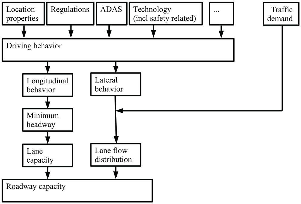
Dependencies leading to the roadway capacity.

User behavior can also vary as a function of time, as can capacity. Obviously, many things have changed since the first report on the fundamental diagram ( 8 ). Cars and technology (engine power, brakes) have changed, but so too have the drivers (who are more used to crowded conditions), and perhaps the driver assistance systems.

A large body of literature has gone into quantifying driver modeling. For instance, Hoogendoorn and Botma discuss how the distribution of individual headways can be modeled and lead to a distribution of closest headways, and thus to capacity ( 9 ). In the same line, Long shows how queue discharge rate relate to various parameters of driving behavior and how this can be derived from field measurements ( 10 ). Which factors ultimately determine the (closest) headway chosen by individuals, was analyzed by Brackstone et al., in their analysis of 123 drivers ( 11 ). Vehicle type was found to be a relevant parameter, but headways were also found to change from day to day. More recently, this domain has been changing: rather than studying the behavior of drivers, it is now the impact of automated vehicles on capacity that is being studied. There are many scientific works on this domain, which use analytical expressions (e.g., Chen et al. [ 12 ], Han and Ahn [ 13 ]), simulations (e.g., Calvert et al. [ 14 ]), and even naturalistic data of drivers (e.g., Schakel et al. [ 15 ]) and of automated vehicles only (e.g., Makridis et al. [ 16 ], Ciuffo et al. [ 17 ], Gunter et al. [ 18 ]).

The current study aimed to directly show the change in capacity over time as a function of changed behavior including all effects (driver behavior, technological changes, and other effects). By doing so, we include all changes, but do not attribute them to a specific source. The current study investigated the effective changes in capacity over the last decade for the same road layout; the study had two goals: (1) to produce findings that could be used in policy analyses for road planning and (2) provide a reference for (weakly/roughly) validation studies aim to describe the same effects reasoned from the perspective of vehicle technology. To this end, we studied capacity conditions in the roadway network and analyzed the collective properties of the traffic stream.

In this paper, the word flow means the passing rate of traffic per unit of time, which in other works is also referred to as volume or intensity. Conceptually, in this paper we differentiate between free flow capacity, that is, the capacity (or maximum flow) before congestion sets in, and the queue discharge rate, which is the maximum flow out of congestion. The difference between the two is the extensively studied capacity drop ( 19 – 21 ). The sequel to this paper will show that it is important to distinguish between the two, since they evolve in a different way. Conceptually, the two are different since the free flow capacity determines when congestion starts, and the queue discharge rate determines the outflow of congestion. We have an interest in this because of the relation to travel time, and for the purpose of planning a road network with appropriate capacities.

Capacity is not a fixed value, not even in the short term (minutes). Because it is result of driving behavior, it fluctuates with the drivers present at that particular moment. For the queue discharge rate, the mean value is most relevant, since the mean over a period multiplied by the duration shows how many vehicles have exited the queue. However, this is different for free flow capacity. Brilon et al. discuss the concept of stochastic (free flow) capacity: there is a probability that traffic can be in free flow conditions at a particular demand level ( 22 ). The difference with queue discharge rate is that once the free flow capacity value is exceeded, traffic breaks down and enters a congested state. Traffic can no longer operate at (free flow) capacity and the outflow reduces to the queue discharge. Flow remains at this (lower) value even if the free flow capacity would have increased again (but traffic cannot reach this free flow capacity state anymore). Therefore, for free flow capacity, not only is the mean relevant, but also the spread and in particular the low-end value of the distribution, since the low-end values are the only flows that can be sustained.

Shiomi et al. also studied long-term changes in capacity ( 23 ). They studied the capacity changes of nine bottlenecks in Japan. They found that the median free flow capacity decreased over time, and that the free flow capacity spread (5th to 50th percentile) also decreased over time, yet was statistically insignificant. No significant changes have been found for queue discharge rate. In a study by Ros et al., most (seven of out nine) bottlenecks were sag sections, which are known to cause congestion and stop-and-go waves ( 24 ). This type of bottleneck rarely occurs in the Netherlands, where bottlenecks mainly consist of lane drops, merging sections, or a combination of the two. They hypothesized that vehicle type (in particular a larger fraction of hybrid vehicles, i.e. vehicles combining a combustion engine with an electric motor), driving behavior, and/or driver assistance systems might have played a role.

In conclusion, we see that there are day-to-day and stochastic fluctuations in free flow capacity and queue discharge rates. However much less is known about long-term changes. For sag sections, a decrease was found for the free flow capacity, but no statistically significant change was found for the queue discharge rate. The gap the current research aimed at was therefore to find how the free flow capacity and the queue discharge rate evolve as a function of the time required for merging and/or lane drop sections. Since the queue discharge rate is expected to fluctuate, we need to analyse a large number of bottlenecks and over a longer time in order to find statistically significant effects.

To study the long-term effects of time on capacity, we considered two approaches. First, we checked locations that had not changed for a long time and, during that time, had formed bottlenecks. There were not many such sites, since bottleneck locations are usually reconstructed to increase their structural capacity. A second approach was to consider the capacity at various bottlenecks that had changed over time, and to correct for the other changes. In the second approach, capacity value is dependent on various explanatory variables (for instance speed limit, number of lanes), as well as time. Changes in road properties should therefore be captured by the explanatory variables, which allow the independent assessment of the autonomous changes of capacity as a function of time. We applied both approaches. The next section will first present the analyses for free flow and queue discharge rate on bottlenecks that have not changed over time. Then we will present the results of a multivariate regression analysis that was undertaken on 143 bottlenecks. The final section discusses both the analyses and results together, and provides the conclusions and a discussion of our findings.

Long-Term Analyses on Selected Bottlenecks

This section will present an analysis of the capacity change (free flow and queue discharge rate) found at sites that have been bottlenecks for a long period (up to 10 years).

Methodology

We studied the evolution of the free flow capacity and the queue discharge rate over a long period. Both capacities were estimated using different methods. This section will first describe the estimation of free flow capacity, and then of the queue discharge rate.

Free Flow Capacity

To estimate free flow capacity, we needed to find the maximum flow possible over a road section before congestion sets in. A higher inflow will cause congestion, and the outflow will be lower (the so-called capacity drop). In idealized conditions with a gradually increasing flow and a deterministic capacity, one can find the value of free flow capacity at only one moment in time: the flow just before the traffic breaks down. Later measurements will give information on the queue discharge rate and are therefore unsuitable for the free flow capacity.

The above description, ignoring stochastic fluctuations, however is not realistic enough in capacity, may be a slightly simplified approach. In this study, we followed the principles laid out by Brilon et al. ( 22 ). This assumes that the capacity, $c$ , is a stochastic value with mean, $μ_{c}$ , and a spread around that: the traffic flow can exceed $μ_{c}$ for a while, whereas a lower flow might cause a breakdown later. The traffic process can consequently be seen as a survival process: how likely it is that traffic can continue to operate without a breakdown. This probability can be calculated, and with it the probability that a traffic jam will arise (i.e., a breakdown).

To compute the probability, we first divided the data into different classes. This was done based on the speed of traffic upstream and downstream of the bottleneck. A measurement period can be classified as,

Free flow (F): if traffic in the current and next period has a high speed both upstream and downstream. One knows that flow measured during this period is below the capacity, but one does not know how much higher the capacity value could be.

Congestion caused by the bottleneck (C): if the traffic has a low speed upstream in the current and previous period, and a high speed downstream. One knows that the bottleneck is causing the queue, but a queue discharge rate is measured and not a free flow capacity. It is not therefore useful for the free flow capacity.

Transition to congestion resulting from traffic demand (B): if the traffic in the current period has a high speed upstream and downstream, but in the next period a low speed upstream and a high speed downstream. One knows that the capacity value is lower than this value, but not by how much.

Congestion caused by a bottleneck downstream (spillback): if the traffic in the current period has a low speed downstream and a high speed upstream, and in the next period a low speed upstream and downstream. These measurements have nothing to do with the capacity of the bottleneck itself, but with another capacity constraint from downstream. They are therefore discarded from further analyses.

To determine the capacity of a bottleneck, we can look at how often traffic flow reaches a certain value, and how often that causes traffic jams. This is a Kaplan–Meier survival analysis. Following Brilon et al. ( 22 ), we defined the function, $F_{c}$ , which describes the (cumulative) probability distribution function for the capacity,

F_{c} (q) = 1 - \underset{i : q_{i} \leq q}{Π} \frac{k_{i} - d_{i}}{k_{i}}; i \in B

(1)

where

$F_{c} (q)$ = unknown cumulative distribution function of capacity $c$ ,

$q$ = traffic flow (vehicles per hour [vph]),

$q_{i}$ = traffic flow in period $i$ (vph),

$k_{i}$ = number of intervals with a flow $q \geq q_{i}$ (-)

$d_{i}$ = number of intervals in which congestion starts at $q_{i}$ (-), and

$B$ = set of intervals where congestion starts at the bottleneck.

This function (1) was only evaluated at the values for which at least one flow value was measured. With discrete flow values (minute-aggregated), we only evaluated the functions at multiples of 60 vph.

For the theoretical foundation, we referred to Brilon et al. ( 22 ). The short and intuitive interpretation of the equation is as follows. The function, $F$ , indicates the breakdown probability of a certain flow. A breakdown can be considered the inverse of a survival (i.e., a breakdown does not occur for a certain flow), denoted $S$ . The survival function, $S$ , is therefore 1 minus the breakdown function, $F = 1 - S$ . This survival probability is computed according to (a) how likely it is that the flow will not break down once it has reached this high level or higher. This is empirically determined by $(k_{i} - d_{i}) / k_{i}$ . The other element (b) of the survival function is that the flow should not have broken down already at lower flows (product of the survival rate for lower flows). Equation 1 can be broken down as follows:

F_{c} (q) = \underset{No breakdown up to flow q}{\underset{︸}{1 - \underset{Survival of flows up to q}{\underset{︸}{\underset{i : q_{i} \leq q}{Π} \underset{Survival of flow q_{i}}{\underset{︸}{\frac{k_{i} - d_{i}}{k_{i}}}} i \in B}}}}

(2)

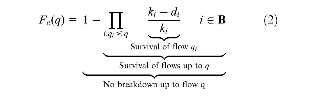
This function does not change if the total amount of collected data changes (i.e., one would collect 10 times as much data with the same underlying distributions).

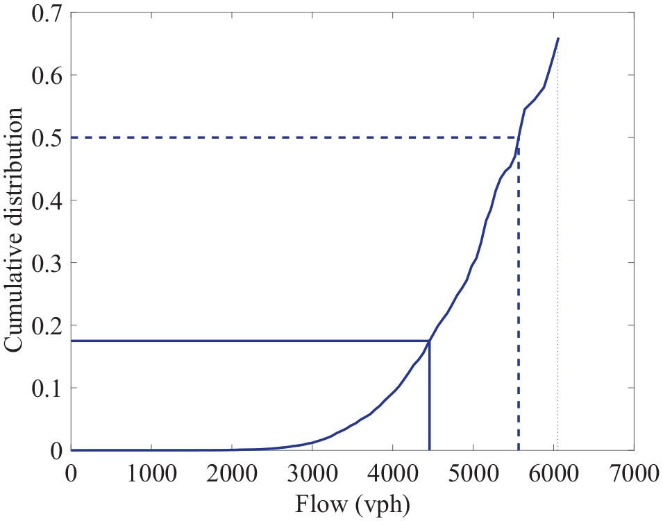
Figure 2 shows an example of this empirical capacity function. For this figure, we include all aggregation periods within a year around June 2016 in which traffic jams occurred were included within a year around June 2016. In this case, the distribution function was created based on 1,123 measurement values of the capacity (i.e., the number of elements in B) combined with 16,734 measurements of flow, which was smaller than the capacity (i.e., the number of elements in F).

Figure 2.

Distribution function of capacities for the measurement periods June 2015 to June 2017.

In many cases, as here, this empirical cumulative probability distribution function will not reach 1. This is because there are periods in which flow exceeds the highest values of flow in set B. Let us consider the example in Figure 2. Here, the highest flow causing congestion was found at approximately 6,050 vph; in other periods, higher flows were measured without causing congestion. In further analyses, we will consider the median of the distribution function for all periods, as well as its 17.5 percentile value. The 17.5 percentile value was chosen because this value is probably found more often, and it corresponds to an inflection point of the probability density function of a normally distributed variable (i.e., mean minus standard deviation).

When determining capacities in this way, several measurements of congestion caused by the bottleneck are required—in the order of hundreds. We were interested in the time evolution, meaning we needed (some percentile value of) a distribution at one point in time. However, recall that one peak hour typically only gives one value, which is insufficient to obtain its full distribution function. To visualize the time evolution of the capacity, a 2-year time window was determined at the start of each month. This way, for all months, a distribution could be found with a moving time window of 2 years. Subsequently, the resulting median and percentile values were taken for the trend analysis. The relative changes for the median and the 17.5th percentile indicate whether the spread of capacity has been increasing or decreasing.

Data aggregated over 1 min were used, which is closest to the data we get. A shorter aggregation interval has the advantage that there are less “mixtures” of states. For example, a longer interval (Interval 1) that is initially not congested, but then is congested, might be classified as not congested. Then, the next interval (Inteval 2) is congested and the flow in interval 1 is now considered to be a breakdown flow, whereas it was only partially the high flow that caused the breakdown. The disadvantage of a shorter interval is that the flows are more volatile, and there might be more intervals with high flows that do not cause a breakdown because of random effects. This means that a shorter interval is likely to lead to a distribution function that ends at a lower maximum percentile value.

For the trend analysis, we included a piecewise linear fit through capacity values as a function of time, for which we used the median and 17.5th percentile values respectively. The slope of this line indicates an increase or decrease in capacity. The fitting function automatically minimizes the error between the fitted line and the measurements, yet additional breaks (more pieces of the piecewise linear fit) incur a penalty. The main goal of the fit is to provide a visual aid. For clarity, we report fitness (root mean squared error).

Queue Discharge Rate

Determining the queue discharge rate is simpler: all flow measurements at the bottleneck (or the first location downstream thereof) during the time that congestion is present are measurements of the queue discharge rate. So all measurements of Class C defined in the previous section are being used. Typically, there are many more data points for the queue discharge rate (class C) than for breakdown flows (class B). One hour of congestion would lead to 60 usable 1-min points.

In this study, we used 1-min intervals since they are most commonly used and this was the base unit of data available (i.e., shorter periods were not possible). Shorter periods yield higher variation, and longer periods lower variation. Note, moreover, that longer periods would be less specific in determining the presence of congestion. For instance, if 15-min periods were used, and 10 out of the 15 min were congested, this 15-minute aggregate data should not be used. Nevertheless, the average speed in the interval could still be below the threshold and so would still be classified as congested owing to the bottleneck. A final remark: the length of the interval will not influence the mean flow.

We hence use short aggregation times of 1 minute. Yet, this will give many observations. To identify the trend, we clustered the observations in bins. We needed to balance a sufficient time resolution (small bin sizes) and sufficient observations per bin (a reliable bin average). The number of bins we choose was the square root of the number of aggregation periods.

To obtain the trend in the queue discharge rate, we fitted a piecewise linear curve through the median flows, for which the same technique was used as for the free flow capacities.

Locations and Data

To obtain the data, we needed a location that (a) would not change in configuration over the long term and (b) forms a bottleneck in the road network. With regard to duration, we considered 10 years to avoid random fluctuations from year to year. Such sites are rare because bottleneck locations are typically one of the first to be improved in a network.

For this research we identified three locations that fulfilled the criteria. Speed contour plots of typical days can be seen in Figure 3.

Figure 3.

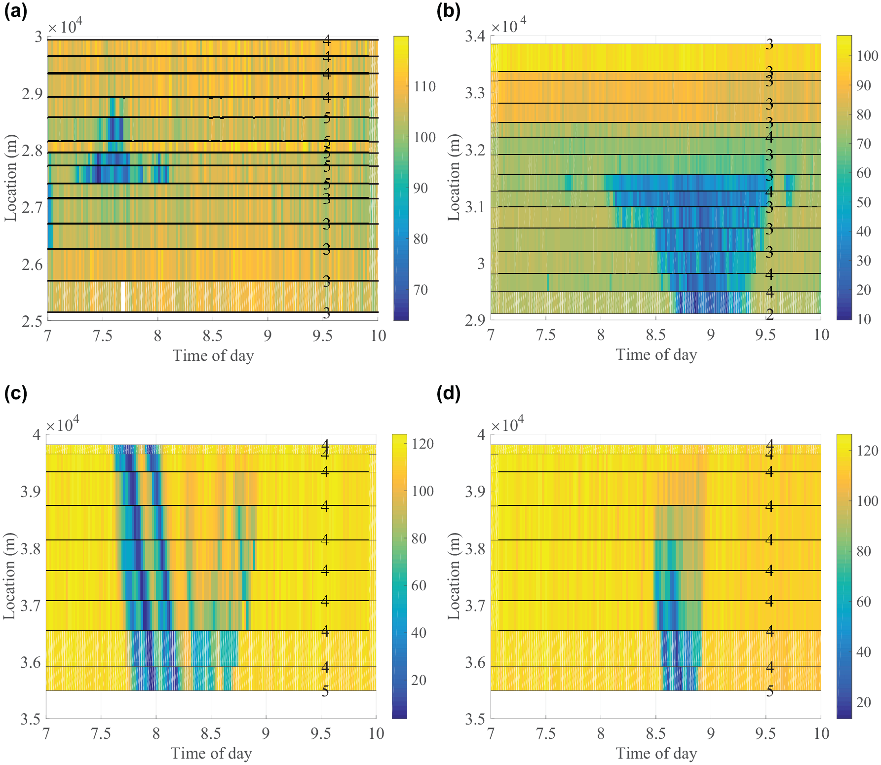
Speed contour plot for the various locations; the digits show the number of lanes: (a) Location 1: a clear traffic jam caused by the bottleneck (traffic direction top to bottom); (b) Location 2: a clear traffic jam caused by the bottleneck (traffic direction bottom to top); (c) Location 3: induced traffic jam (traffic direction bottom to top); and (d) Location 3: no clear bottleneck location (traffic direction bottom to top).

The first location is the A12 motorway near the Dutch town Gouda in a westbound direction. The weaving section upstream of the lane drop and motorway diverge form a bottleneck. The second location is the A20 motorway near the city of Rotterdam in a westbound direction. The bottleneck is formed by the motorway junction for Rotterdam city center (three-lane freeway). The third location is the A12 motorway near the onramp for Bodegraven in an eastbound direction. The large inflow from the N11 without an increase in the number of lanes (four lanes) forms the bottleneck. Location 3 has only been a bottleneck since 2013; queuing is not always apparent at the bottleneck location, as Figure 3, c and d , show. The speed limit is different for each location. To avoid false positives in congestion detection, we adapted the threshold value to distinguish congestion from free flow to the location: 80, 65, and 85 km/h, respectively, for the three locations. Note that the days for which queuing was not clearly caused by the bottleneck were filtered out by the classification described in the Methodology section.

The Dutch freeway network is equipped with double loop detectors at approximately 500-m distances. Data were saved in an aggregate form, at aggregation intervals of 1 min, providing lane-specific mean speeds, and flows. We added the flows and computed the harmonically weighted average of the time mean speeds of the different lanes. Since speeds per lane are more homogeneous than speeds across the roadway, this provides a more accurate approximation of Edie’s mean speed ( 25 ) (which is completely accurate if the speeds within a lane are homogeneous) ( 26 ).

Data over a road stretch of 5 km per bottleneck location were requested, allowing for a slight variation in the head of the queue. Note, moreover, that within the observed period the road layout did not change, but the detector configuration did, which was also a reason for analyzing a longer road stretch. The time interval was March 2006 to October 2017. This allowed for 10 years of observations, including the moving average of 1 year. For all week days (Monday through Friday), data from 7 to 10 a.m. were requested; this time interval included the full morning peak congestion. For the remainder of the analysis, we used the data that were present and valid (sometimes detectors fail or prove unreliable).

Figure 4 shows the results for the evolution of the free flow capacity (left column) and the queue discharge rate (right column) for all three locations. We will discuss them in turn, in the order of location. Note that to better illustrate the changes in capacity, the scale is adapted per subfigure.

Figure 4.

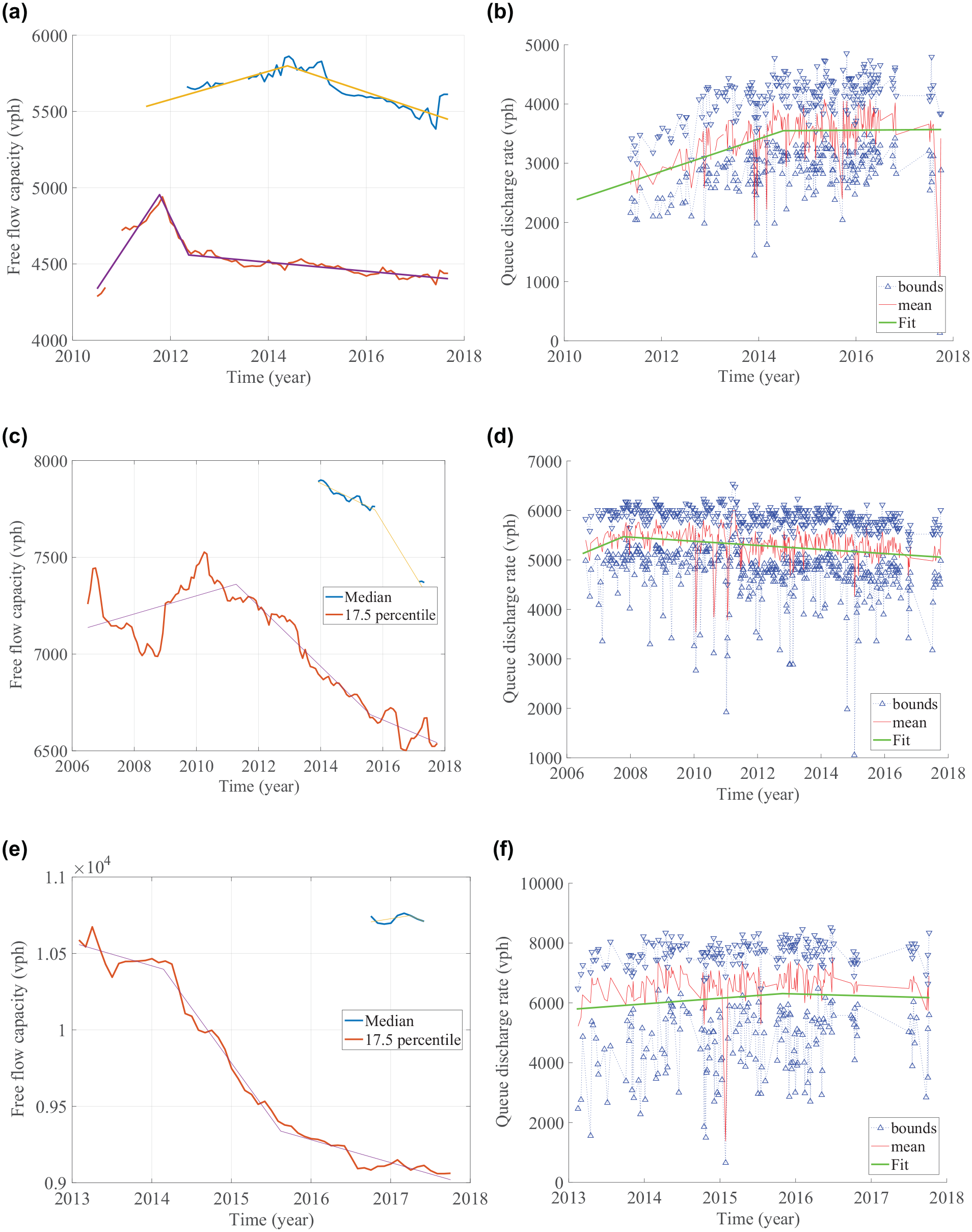
Evolution of the capacity at individual locations: (a) Location 1 free flow capacity, (b) Location 1 queue discharge rate, (c) Location 2 free flow capacity, (d) Location 2 queue discharge rate, (e) Location 3 free flow capacity, and (f) Location 3 queue discharge rate.

Results

At Location 1, the free flow capacity seemed to have a brief peak, probably caused by limited congestion measurements from before 2011. The reduction of free capacity from 2012 (17.5th percentile value) or 2014 (median) was clearer. The free flow capacity decreased with 30 vph (17.5th percentile) and 110 vph (median) per year (for three lanes). Owing to the nature of these measurements (one every minute of congestion), the values for the queue discharge rate were much more volatile. The queue discharge rate showed an increase up to 2014, after which it was more or less constant (annual increase of 6 vph).

Location 2 showed no clear trend until 2011 (the fit showed an increase, but several trends could be seen as well). Later, from 2010 to 2011, a decrease of the 17.5th percentile value as well of as of the free capacity was seen, with a decrease of 260 (17.5th percentile), 160 (2011 to 2015), and 70 vph (2015 to 2017). The queue discharge rate capacity seemed to increase a little in the first year (+260 vph in 1.3 years), but showed a decreasing trend from 2012 (annual reduction of 41 vph from August 2008 to November 2017).

For Location 3, capacity measurements were only possible from 2013. Since then, the free flow capacity (17.5th percentile value) has been decreasing. The median of free capacity was found only in a few measurement periods, so it was not possible to identify a trend. The queue discharge rate hardly varied over time. The best fit indicated that this first increased and then decreased, but the effects (i.e., increase or decrease) did not exceed the bounds.

Overall, we observed that a possible trend of increasing free flow capacity seemed to change to a decreasing free flow capacity over the last 5 years. This change in trends is a clear and relevant finding. For the queue discharge rate the results were not as clear: the increase fell within the bounds. For the queue discharge rate, further analysis of more locations and factors was therefore carried out and is presented in the next section.

Evolution of Capacities: Exogenous Factors

Apart from locations that are bottlenecks and that have not changed, we also considered capacity at a variety of locations where we corrected for the change in location properties.

Data

The basis for this analyses was a data set containing traffic data of 143 locations throughout the country. This database was available because it had been compiled by the Dutch Road Authority for the evaluation of previous capacity studies. The data cover the period 2011 to 2015. The locations are shown in Figure 5; most indicated sites provide data for traffic in both directions. Contrary to previous analyses, here we used data from only one detector. Because we did not have data from detectors upstream and downstream, we could not apply the same classification techniques as in the previous section. The methodology we used is explained in the next section, followed by a description of the results

Figure 5.

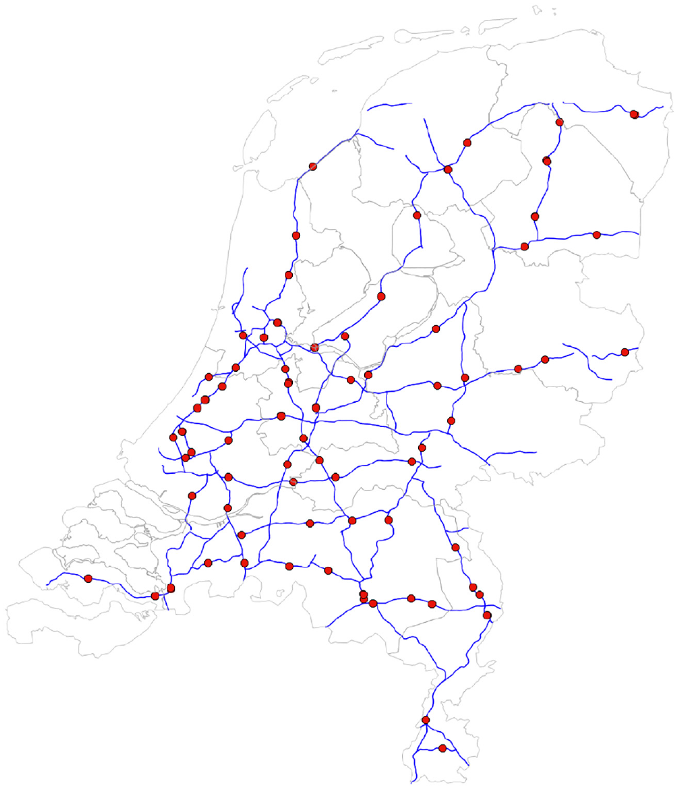
Locations of the measurement points on a map of the Netherlands. All locations are used in both directions.

Methodology

We based our analysis on the raw data obtained from double loop detectors. Inclusion criteria for the relevant aggregation periods were based on what was expected for the driving behavior, and the individual spacing, $s$ . Our basic idea was that a simplified speed-dependent spacing might follow the equation

s^{*} (v) = s_{0} + Tv

(3)

where

$v$ = speed,

$T$ = net time headway, and

$s_{0}$ = effective vehicle length.

Note, we used this equation for the selection criteria only, and if driving behavior differed, this did not influence the outcomes.We filtered out the period outliers based on the speed–spacing relationship. We excluded periods in which the spacing was either too small, $s < s^{*} (v)$ , with $s_{0}$ = 0 and $T = 0.9$ s; or too large, $s > s^{*} (v)$ with $s_{0}$ = 20 m and $T = 4.5$ s. These measurements would not be part of normal traffic operations. Moreover, since we were only interested in congested times, we filtered out periods with speeds that were too high, $v > v_{0}$ , with $v_{0}$ = 65 km/h. We took a lower speed separation value here to avoid including periods in which speed was low because of reasons other than congestion. Since this was a one-detector filtering (rather than the two-detector filtering described in the previous section), the threshold set was a little stricter. The whole procedure gave the flows in periods where there was congestion. We know that the flow in congestion is equal to the flow through the bottleneck, which is with an activated bottleneck the queue discharge rate.

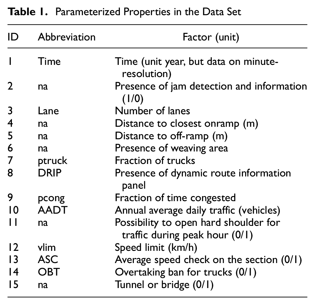
Using the above filters, we found (a series of) values for the queue discharge rate for each site. Via a multivariate regression analysis we aimed to approximate the queue discharge rate as a function of the properties of the site. The available properties and their parametrization are listed in Table 1. For the parameters that were subsequently found to be statistically significant (see Table 2), an abbreviation is also included.

Table 1.

Parameterized Properties in the Data Set

ID	Abbreviation	Factor (unit)
1	Time	Time (unit year, but data on minute-resolution)
2	na	Presence of jam detection and information (1/0)
3	Lane	Number of lanes
4	na	Distance to closest onramp (m)
5	na	Distance to off-ramp (m)
6	na	Presence of weaving area
7	ptruck	Fraction of trucks
8	DRIP	Presence of dynamic route information panel
9	pcong	Fraction of time congested
10	AADT	Annual average daily traffic (vehicles)
11	na	Possibility to open hard shoulder for traffic during peak hour (0/1)
12	vlim	Speed limit (km/h)
13	ASC	Average speed check on the section (0/1)
14	OBT	Overtaking ban for trucks (0/1)
15	na	Tunnel or bridge (0/1)

Table 2.

The Parameter Estimates

	Constant	$c_{1}$	$c_{3}$	$c_{7}$	$c_{8}$	$c_{9}$	$c_{10}$	$c_{12}$	$c_{13}$	$c_{14}$
		Time	Lane	ptruck	DRIP	pcong	AADT	vlim	ASC	OBT
Value $c_{i}$	2,296	45	−257	−2,222	−173	7,5E3	41	−8	−757	130
t-value	7.3	3.0	−7.0	−8.8	−2.0	8.2	7.6	−3.1	−3.9	3.8

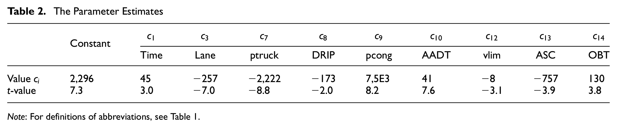
Note: For definitions of abbreviations, see Table 1.

A part of these properties is dynamic with different timescales. For instance, the truck fraction changes with traffic, and the number of lanes can change over a larger timescale. We therefore adapted the parameters to the period of measurement.

The queue discharge function we estimated was a linear additive function,

c = c_{0} + \sum_{i = 1}^{15} c_{i} p_{i}

(4)

where

$c_{0}$ = base queue discharge rate,

$p_{i}$ = value of the $i$ th variable (from Table 1), and

$c_{i}$ = rate of change of the queue discharge rate with a change of variable.

Note that the variable estimated here, $c$ , was normalized for the number of lanes, and therefore was the queue discharge rate per lane. This allowed for more flexible adaptation to changes in the number of lanes.

The base queue discharge rate, $c_{0}$ , and all 15 values of $c_{i}$ were found by performing a least squares optimization. To have the best matching coefficients for the significant parameters, we iteratively removed the least significant parameter in the fit until the fit only had significant parameters. To assess significance, we used t-value, and a cutoff value of 2 for significance.

Results

The results of the multivariate estimation are given in Table 2. The base queue discharge rate was 2,296 vehicles per hour per lane (vphpl). This result matched the Dutch highway capacity manual well ( 2 ). Before considering the time effect, let us consider the effect of the significant parameters, and in particular the signs. All signs of the parameters were as expected. A higher truck fraction will reduce queue discharge. With a passenger car equivalent value of trucks of approximately 2 ( 27 ), we expected a coefficient in the order of the base queue discharge. This holds in the limit for a truck percentage of 0%. The typical truck percentage was around 5% to 15%. More lanes decreased the queue discharge rate of each lane (by approximately 10% per lane), which was expected owing to inefficient lane usage. A higher speed limit decreases queue discharge; this approach has been the basis for various projects aiming to reduce speed and increase homogeneity; this effect was statistically significant, yet the size of the effect was small ( 28 ). With a higher fraction of congested measurements, the queue discharge rate increased. This was expected since the drivers in these conditions were used to driving in busy conditions and could handle short headways. The coefficient was large because the variation in fractions of congestion were very small (e.g., a change from 1% to 1.5% of the time leads to a change of 0.005 in the variable pcong). For the same reason, the sign of annual average daily traffic (AADT) was positive (drivers on busier sections were used to crowded conditions), and had a low value because the AADT itself was a large number. The presence of a dynamic route information panel was negatively correlated with queue discharge rate, which can be explained by the how these are mostly at locations where drivers need to choose their route, which (a) distracts them from their car-following task ( 29 ), and (b) might cause lane changes owing to a route choice, which induces gaps and reduces the queue discharge rate ( 30 ). The presence of (average) speed checks reduced the use of the left lane; this decreased the overall queue discharge rate. Finally, the presence of an overtaking prohibition for trucks increased the queue discharge rate, which was expected since overtaking slow trucks (speed limit 80 km/h, slower than other traffic with speed limits of 100 to 130 km/h) creates gaps ( 30 ).

The factor time was found to be significant, with an annual increase in capacity of 45 vphpl. Note again that this was the exogenous change in queue discharge rate, which was not explained by any of the other variables in Table 1. Whereas the value of the number might seem small, it was statistically significant. Moreover, over the analyzed period of 5 years, this could change the capacity considerably (10%).

Conclusion and Discussion

This study analyzed the evolution of capacity as a function of time. The main conclusion for the paper was that free flow capacity changes at a different rate than the queue discharge rate, and even in the opposite direction. The free flow capacity was found to have been decreasing and the queue discharge rate increasing over time. This finding could be directly used in policies for road planning.

For further research, a takeaway is that research into the long-term evolution of capacity should study free flow capacity separately from queue discharge rate. The free flow capacity and the queue discharge rate namely have opposite effects on hours, and experience different changes over time.

The changes in capacity were caused by driver behavior, such as car-following or lane choice. However, the underlying cause of these changes is unknown and could not be determined by this empirical work. Causes can range from driver education, vehicle techniques to the state of the economy and environmental awareness. A topic for further research could be to identify the cause of the effects found here. They could potentially originate from different sources, but it would also be possible for them to have originated from one source. Answers may lie beyond the field of traffic engineering, in sociological-, economical-, or ecological-based reasoning.

Nevertheless, we would like to posit one hypothesis in the area of traffic engineering: the effect of Adaptive Cruise Control (ACC) systems. These could potentially be the underlying cause of both the decrease of the free flow capacity and the increase of the queue discharge rate. Early ACC systems worked in high-speed conditions (i.e., free flow) and disengaged at low speeds (therefore, queue discharge rate was unaffected). Moreover, it is known that ACC maintains longer headways than human drivers in the Netherlands ( 31 ), and these systems (used to) switch off at low speeds. This could mean that the reduction in free capacity could be a result of the use of high-speed ACC systems. It could even be possible that recent ACC systems have a different impact than older systems because they operate at all speeds, and therefore also might affect the queue discharge rate. In the most modern systems, studies have found that reaction times are longer than human reaction times ( 16 , 32 ).

The current study could provide empirical background for other studies exploring the effects of ACC systems reasoned from the individual vehicle (i.e., up-scaling results obtained from one or a couple of vehicles). Proving this hypothesis from a collective traffic perspective (rather than individual vehicles) would be challenging. One reason is that even if penetration rates of the vehicle fleet are known, this would still give insufficient information on the presence of such systems that are active during peak hours. With a known static penetration rate, the fraction of the vehicles on the road ACC equipped vehicles would still be unknown (however, this might be different because one type of car might be used more frequently, or more in specific conditions). Even if known, the fraction of drivers actively using ACC systems would still be unknown. An in-vehicle analysis would be required.

An alternative hypothesis of changed driver behavior relates to increased driver distraction. This could lead to increases in reaction time, which would specifically decrease the queue discharge rate. Note again that these are unconfirmed hypotheses posited by the authors and causes may well lie in other domains, potentially even beyond traffic engineering. Testing these or other hypotheses relating to the potential causes of the empirically revealed changes in free flow capacity and queue discharge rate is a topic for further research.

Footnotes

Author Contributions

The authors confirm contribution to the paper as follows: study conception and design: V.L. Knoop and S.P. Hoogendoorn; data collection: V.L. Knoop and S.P. Hoogendoorn; analysis and interpretation of results: V.L. Knoop and S.P. Hoogendoorn; draft manuscript preparation: V.L. Knoop. All authors reviewed the results and approved the final version of the manuscript.

Declaration of Conflicting Interests

The authors declared no potential conflicts of interest with respect to the research, authorship, and/or publication of this article.

Funding

The authors disclosed receipt of the following financial support for the research, authorship, and/or publication of this article: This research was sponsored by the KiM Netherlands Institute for Transport Policy Analysis.

ORCID iDs

Victor Knoop

Serge Hoogendoorn

References

Highway Capacity Manual . Transportation Research Board, Washington, D.C., 2016.

Dienst Water, Verkeer en Leefomgeving. Capaciteitswaarden Infrastructuur Autosnelwegen (Capacity Values Infrastructure Freeways, in Dutch). Tech. rep., Rijkswaterstaat, Dutch Road Authority, 2015.

Shaout

Colella

Awad

Advanced Driver Assistance Systems-Past, Present and Future. Proc., 7th International Computer Engineering Conference (ICENCO’2011), Cairo, Egypt, IEEE, 2011, pp. 72–82.

Ossen

S. J. L.

Longitudinal Driving Behavior: Theory and Empirics. Trail thesis series. Delft University of Technology, Netherlands, 2008.

Kesting

Treiber

Helbing

Enhanced Intelligent Driver Model to Access the Impact of Driving Strategies on Traffic Capacity. Philosophical Transactions of the Royal Society of London A: Mathematical, Physical and Engineering Sciences, Vol. 368, No. 1928, 2010, pp. 4585–4605.

Dervisoglu

Gomes

Kwon

Horowitz

Varaiya

Automatic Calibration of the Fundamental Diagram and Empirical Observations on Capacity. Proc., of the Annual Meeting, Washington, D.C., 2009.

Knoop

V. L.

Daamen

Automatic Fitting Procedure for the Fundamental Diagram. Transportmetrica B: Transport Dynamics, Vol. 5, No. 2, 2017, pp. 129–144.

Greenshields

B. D.

A Study of Traffic Capacity. Proceedings Highway Research Board, Vol. 14, 1934, pp. 448–477.

Hoogendoorn

S. P.

Botma

Modeling and Estimation of Headway Distributions. Transportation Research Record: Journal of the Transportation Research Board, 1997. 1591: 14–22.

10.

Long

Driver Behavior Model of Saturation Flow. Transportation Research Record: Journal of the Transportation Research Board, 2007. 2027: 65–72.

11.

Brackstone

Waterson

McDonald

Determinants of Following Headway in Congested Traffic. Transportation Research Part F: Traffic Psychology and Behaviour, Vol. 12, No. 2, 2009, pp. 131–142.

12.

Chen

Ahn

Chitturi

Noyce

D. A.

Towards Vehicle Automation: Roadway Capacity Formulation for Traffic Mixed With Regular and Automated Vehicles. Transportation Research Part B: Methodological, Vol. 100, 2017, pp. 196–221.

13.

Han

Ahn

Stochastic Modeling of Breakdown at Freeway Merge Bottleneck and Traffic Control Method Using Connected Automated Vehicle. Transportation Research Part B: Methodological, Vol. 107, 2018, pp. 146–166.

14.

Calvert

Schakel

VanLint

Will Automated Vehicles Negatively Impact Traffic Flow?

Journal of Advanced Transportation, Vol. 2017, 2017, p. 3082781.

15.

Schakel

W. J.

Gorter

C. M.

De Winter

J. C.

Van Arem

Driving Characteristics and Adaptive Cruise Control? A Naturalistic Driving Study. IEEE Intelligent Transportation Systems Magazine, Vol. 9, No. 2, 2017, pp. 17–24.

16.

Makridis

Mattas

Anesiadou

Ciuffo

OpenACC. An Open Database of Car-Following Experiments to Study the Properties of Commercial ACC Systems. Transportation Research Part C: Emerging Technologies, Vol. 125, 2021, p. 103047.

17.

Ciuffo

Mattas

Makridis

Albano

Anesiadou

Josvai

Komnos

Pataki

Vass

, et al. Requiem on the Positive Effects of Commercial Adaptive Cruise Control on Motorway Traffic and Recommendations for Future Automated Driving Systems. Transportation Research Part C: Emerging Technologies, Vol. 130, 2021, p. 103305.

18.

Gunter

Gloudemans

Stern

R. E.

McQuade

Bhadani

Bunting

Delle Monache

M. L.

, et al. Are Commercially Implemented Adaptive Cruise Control Systems String Stable? IEEE Transactions on Intelligent Transportation Systems. Vol. 22, No. 11, 2021, pp. 6992–7003.

19.

Hall

F. L.

Agyemang-Duah

Freeway Capacity Drop and the Definition of Capacity. Transportation Research Record: Journal of the Transportation Research Board, 1991. 1320: 91–98.

20.

Cassidy

Bertini

Some Traffic Features at Freeway Bottlenecks. Transportation Research Part B: Methodological, Vol. 33, No. 1, 1999, pp. 25–42.

21.

Yuan

Capacity Drop on Freeways: Traffic Dynamics, Theory and Modeling. PhD thesis. Delft University of Technology, Netherlands, 2016.

22.

Brilon

Geistefeldt

Regler

Reliability of Freeway Traffic Flow: A Stochastic Concept of Capacity. Proc., 16th International Symposium on Transportation and Traffic Theory, College Park, MD, 2005, pp. 125–144.

23.

Shiomi

Xing

Kai

Katayama

Analysis of the Long-Term Variations in Traffic Capacity at Freeway Bottleneck. Transportation Research Record: Journal of the Transportation Research Board, 2019. 2673: 390–401.

24.

Ros

B. G.

Knoop

V. L.

van Arem

Hoogendoorn

S. P.

Empirical Analysis of the Causes of Stop-and-Go Waves at Sags. IET Intelligent Transport Systems, Vol. 8, No. 5, 2014, pp. 499–506.

25.

Edie

Discussion of Traffic Stream Measurements and Definitions. Proc., 2nd International Symposium on the Theory of Traffic Flow, OECD, Paris, France, 1965.

26.

Knoop

V. L.

Hoogendoorn

S. P.

Van Zuylen

H. J.

Empirical Differences Between Time Mean Speed and Space Mean Speed. Proc., Traffic and Granular Flow 07, Springer, Paris, France, 2007.

27.

Dutch Road Authority. Capaciteitswaarden Infrastructuur Autosnelwegen. Tech. rep., Rijkswaterstaat, 2011.

28.

Hoogendoorn

Daamen

Hoogendoorn

Goemans

Assessment of Dynamic Speed Limits on Freeway A20 Near Rotterdam, Netherlands. Transportation Research Record: Journal of the Transportation Research Board, 2013. 2380: 61–71.

29.

Hoogendoorn

S. P.

Brookhuis

Daamen

Mental Workload, Longitudinal Driving Behavior, and Adequacy of Car-Following Models for Incidents in Other Driving Lane. Transportation Research Record: Journal of the Transportation Research Board, 2010. 2188: 64–73.

30.

Laval

J. A.

Daganzo

C. F.

Lane-Changing in Traffic Streams. Transportation Research Part B: Methodological, Vol. 40, No. 3, 2006, pp. 251–264. https://doi.org/10.1016/j.trb.2005.04.003.

31.

Viti

Hoogendoorn

S. P.

Alkim

T. P.

Bootsma

Driving Behavior Interaction With ACC: Results from a Field Operational Test in The Netherlands. Proc., Intelligent Vehicles Symposium, Eindhoven, Netherlands, IEEE, 2008, pp. 745–750.

32.

Lanaud

Ladino

Buisson

First Observations About Response Times and Connectivity in a Vehicles Platooning Experiment. Transport Findings, 2021. http://doi.org/10.21949/1504485.

Free Flow Capacity and Queue Discharge Rate: Long-Term Changes

Abstract

Keywords

Long-Term Analyses on Selected Bottlenecks

Methodology

Free Flow Capacity

Queue Discharge Rate

Locations and Data

Results

Evolution of Capacities: Exogenous Factors

Data

Methodology

Results

Conclusion and Discussion

Footnotes

Author Contributions

Declaration of Conflicting Interests

Funding

ORCID iDs

References