
Abstract
The MOBIS-Covid data provides a unique opportunity to put mobility adjustments observed during the crisis in perspective. A large panel has been tracked from before the crisis up until the end of 2022. Starting with 1370 participants and observing a gradual drop-off, around 250 kept tracking throughout the whole study period of over 2 years. Switzerland lifted its measures counteracting the virus spread in mid-February 2022, reaching a potential new equilibrium in the months after. Descriptive indicators have been constructed for Switzerland in order to disentangle the narrative of the crisis from the perspective of transport demand. The descriptive findings are supplemented by a mixed multiple discrete-continuous extreme value model (MMDCEV). We find a shift in modal splits away from car and train, where in particular bus could expand its mode share. While the cycling and walking booms were temporary, the bicycle still shows slightly higher mode distance shares. There are observable differences between the working arrangements (home office, mixture and in-office), however, we do not find evidence that preferences differ substantially. This suggests that the working arrangement segments the population along socioeconomic dimensions with different mobility behaviors and mode preferences. Modes are more satiated in the post-pandemic world, hinting that people use fewer modes in their weekly modal mix but use them more intensely. However, the model suggests that the pandemic should not be read as a structural break in mode preferences. We will therefore likely see further convergence to the pre-pandemic equilibrium.
Keywords
The COVID pandemic hit our system from various angles. First and foremost, it was a health crisis with risk asymmetries between different groups in society. It was also a considerable shock to our economies, with high uncertainty and supply chains breaking down. Firms proved to be very flexible, adopting working from home and keeping productivity at high levels. Last but not least, the initial solidarity seemed to fade with the duration of the crisis and political polarization peaked with the vaccine roll-out. Not surprisingly, almost all of these dimensions played into our mobility behavior in one way or another, either directly (e.g., because of health concerns) or indirectly (e.g., by reducing commuting activities through working from home).
Several studies have been trying to describe the evolution of transport demand during the early stages of the crisis, using different means such as tracking studies or questionnaires. But of course, all the effects outlined above were intertwined and a clear attribution has been difficult. Therefore, it has not been possible to answer the question of whether or not these patterns have persisted in the post-pandemic world.
The MOBIS-COVID study ( 1 ) provides a unique opportunity to look at the persistence of these effects. A Swiss panel with a rich socioeconomic information set has been tracked from before the crisis until the end of 2022. In Switzerland, all restrictions and measures to contain the spread were lifted on February 17, 2022, and we potentially converged to a new equilibrium in the months that followed. Therefore, we have revisited the MOBIS-COVID data and tried to comment on how sustainable initial findings have proven to be and to translate these to recent times. For this purpose, a comprehensive set of descriptive indicators has been constructed to disentangle the narrative of the crisis. Special emphasis is given to the question of how new hybrid working arrangements (referred to throughout as “home office”) drive modal splits (as measured by mode distance shares). The descriptive findings are strengthened by a mixed multiple discrete-continuous extreme value (MMDCEV) model in which we model both the discrete and the continuous dimension of weekly mode distance shares and compare the pre-pandemic to the arguably post-pandemic world.
COVID-19 Timeline in Switzerland
Based both on the COVID case numbers and the measures imposed to counteract the spread of the virus, the following six phases can be distinguished. The phases are visualized together with COVID case numbers (rolling 14 day mean) in Figure 1. The narrative of the pandemic is presented hereafter and summarized in Table 1, where each phase of restrictions (constraining free movement) is followed by a phase of relaxation.
Phase 1 (restriction): COVID-19 reached Switzerland in early 2020. The situation deteriorated quickly and by March 20, 2020 over 4800 people were infected. This first phase can thus be characterized by a rapid spread of the virus as well as high uncertainty. On March 16, 2020 the Federal Council declared an extraordinary situation, which allowed it to introduce uniform measures in all cantons. A lockdown was imposed, closing all nonessential businesses, along with schools, recreational facilities, and public parks. As a consequence, employers were urged to reorganize the working hours of their employees to avoid peak-hour travel. Home office was implemented, wherever possible. The measures were extended until April 26, 2020, after which the Federal Council followed a strategy to gradually emerge from the lockdown in three stages.
Phase 2 (relaxation): The gradual easing of the enforced measures ended on June 6, 2020, when all events up to 300 people and spontaneous gatherings for up to 30 people were allowed again. High schools and universities were able to resume, and all leisure and entertainment businesses as well as tourist attractions reopened. Relatively calm summer months followed, suggesting that the spread of the virus might follow seasonal patterns.
Phase 3 (restriction): Beginning October 19, 2020, a series of measures was introduced again as the situation worsened. Home office was recommended, culminating in a home-office requirement starting January 18, 2021. The requirement was in place until June 26, 2021.
Phase 4 (relaxation): However, even before abolishing the home-office requirement, other measures constraining the free movement of people were gradually eased as the third COVID wave was rather shallow. That is, while commutes were still reduced during phase 4, leisure activities were not. Again, the summer months were relatively calm.
Phase 5 (restriction): With the onset of autumn at the end of September 2021, the last restrictive phase started. New, aggressive COVID variants emerged. As vaccination was fully rolled out with all residents having had the opportunity to get vaccinated twice, a COVID certificate was required, starting September 13, 2021. Political polarization was a consequence, with society being divided into two segments with different constraints. However, home office became mandatory again for all, as of December 20, 2021 and was in place until February 3, 2022.
Phase 6 (relaxation): Despite rocketing case numbers, the path back to normalization started in February 2022 (as intensive care stations were not at limiting capacities any longer). Almost all measures were abolished by February 17, 2022. As the transition to a relatively normal life might have taken some time, we define the normalization phase to have begun March 1, 2022.
The baseline period is defined as all data points before October 31, 2019. The period from November, 2019 to the onset of the pandemic in late February, 2020 is discarded as a randomized controlled trial was conducted and mobility patterns are expected to have been affected by the treatment.
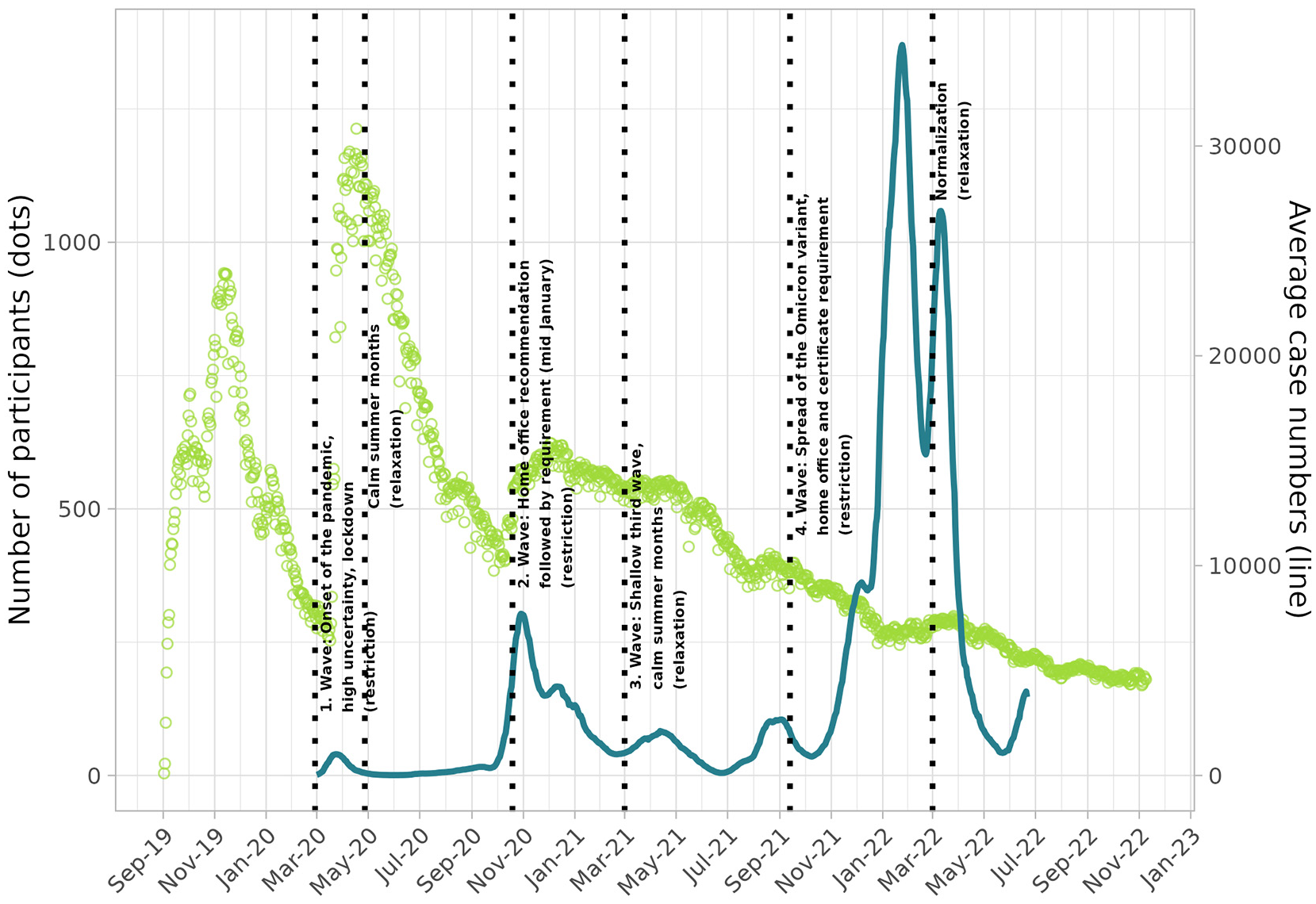
COVID case numbers and timeline.
Evolution of the Pandemic in Six Phases
Note: 2020-02-28 = February 28, 2020.
Related Work
In this section, we review studies that explore the impact of COVID-19 on mobility patterns with a focus on modal shifts. Whereas changes during the pandemic are well understood, literature that looks beyond the crisis is sparse for obvious reasons. Nevertheless, some work has been identified that tries to generalize the initial findings to an environment without COVID restrictions.
Paul et al. ( 2 ) present a review of the global findings on changes in transportation behavior caused by the COVID-19 pandemic. During the pandemic, reduced usage of public transportation could be observed while reliance on private cars increased. While this is a global pattern, nonmotorized vehicle usage and walking prevalence increased mostly in European countries. Trips for some particular purposes remained high, using only a specific mode of transport. Several studies report a decrease in commuting, which can be attributed to either job loss or an increase in working from home. Similarly, sociodemographic attributes determine the trip frequency—mediated by, among other things, home-office access. Risk perceptions play an important role too.
Abdullah et al. ( 3 ) report that trip purpose, mode choice, distance traveled, and frequency of trips were significantly different before and during the pandemic. Shopping trips were the dominant trip-generating purpose. A shift from public transport to private and nonmotorized modes could be observed. This can be attributed to people placing a higher priority on health-related concerns when choosing a mode during the pandemic.
Molloy et al. ( 4 ) use the MOBIS data set ( 1 ) and conduct comprehensive descriptive analysis to report the impact of restrictive measures during the pandemic on mobility behavior. Reductions of around 60% in the average daily distance were observed, with decreases of over 90% for public transport. Meanwhile, the cycling mode share increased drastically. Modal shifts were considerable, especially for public transport subscription holders. The change in modal shares was particularly pronounced when restrictions were imposed and somewhat less so after restrictions were eased. However, pre-pandemic levels were never reached during the study period. The authors further find that home office is effective for suppressing travel demand with effects persisting over the enforced home-office periods. The authors discuss long-term policy implications. However, the time window from the onset of the pandemic until the middle of August 2020 is rather short and extrapolation beyond the pandemic situation has to be seen in that perspective. As we use the same data set and conduct very similar descriptive analysis, our work puts these preliminary findings in context and scrutinizes whether or not the observed changes during the pandemic have become habitual.
Meister et al. ( 5 ) employ an MMDCEV model to estimate mode distance shares for an urban population. Separate parameters were derived for four distinct segments, from September 2019 until the end of 2020 (still amid the crisis). Their findings confirm global trends: a substantial decrease in public transport usage (50% depression at the end of their sample period), recovered car usage (with a temporary increase of 40% during the pandemic), and a cycling boom (increase in travel distance up to 150% and frequency increasing by 40% during summer). The model sheds light on a change in user group composition for public transport (PT) and cycling.
Currie et al. ( 6 ) is one of the few studies that pursue the question of whether post-pandemic travel behavior will be different from pre-pandemic travel. The study relies on data from a survey in which respondents were asked to reveal their future expectations. PT ridership will recover but is not expected to reach pre-pandemic levels. The mode share of cars will increase and offset reduced congestion associated with working from home, resulting in a net increase of car usage and higher peak volumes. Although the study was conducted in Melbourne, the results seem to generalize and support the findings by Shamshiripour et al. ( 7 ) and Beck et al. ( 8 ).
To summarize, the general narrative reveals a modal shift away from PT to car and in particular to nonmotorized forms of transport. Even though home office might reduce peak volumes, congestion might increase because of a net increase in individualized transport. Different sociodemographic groups adjust mode usage differently, mainly because of different risk perceptions (during the pandemic) or home-office access. Previous work either extrapolated findings during the pandemic to the post-pandemic world or relied on respondents’ expectations.
Method
Data
Starting in September 2019, a sample of 5375 Swiss residents were recruited to take part in a mobility-pricing field experiment called MOBIS. Using an app, the participants tracked their location and thereby mobility and activity patterns could be identified. They were tracked for 8 weeks in an attempt to investigate their response to a conceptual mobility-pricing scheme, in a randomized controlled trial. Participation and tracking numbers are depicted in Figure 1, together with COVID case numbers and the six phases outlined before.
The 3680 participants who completed the MOBIS study were asked to reactivate the app in an effort to understand mobility behavior during the pandemic. Around 1400 volunteered to do so, building the panel of the MOBIS-COVID-19 study that is the basis of this report.
People were only eligible to participate in the MOBIS study if they used a car at least 2 days a week. This skewed our sample toward car drivers. However, comparing the sample to the last national travel diary, Mikrozensus (MZ) 2015, the MOBIS-COVID-19 sample was found to be broadly representative of the Swiss population ( 4 ).
After January 2021 we observe a gradual drop-off in participants as no further major recruitment efforts had been made. Nevertheless, around 250 people were still using the app during the normalization period. This raises the concern of a potential self-selection bias. To make statistics comparable over the full time horizon a re-weighting scheme is applied, comparing the characteristics of the remaining individuals against the original 22,000 respondents who filled out the introductory survey. Weights are based on age, gender, income, education, mobility tool ownership, and accessibility and are calculated for each person-week.
The socioeconomic characteristics were collected in several surveys during various stages of the study. While some of the questions were included in several survey instruments, it is important to acknowledge that for most of the variables, we do not have longitudinal information. That is, only one particular point in time is reflected and some of the attributes might have changed over time. For example, the working-arrangement variable {Home office, Mixture, Work outside home} is based on two work-related surveys, fielded in April 2021 (phase 3) and October 2021 (phase 4). Therefore it most certainly happened that some of the people were labeled home working in phase 3 or 4 but switched back to in-office without us noticing.
Descriptive Analysis of Mobility Patterns
In this section, the evolution of different mobility patterns is described. Different correlation patterns shed light on a possible narrative accompanying the evolution during the six phases (see Table 1). We first elaborate on activity spaces before looking at various mode-specific patterns.
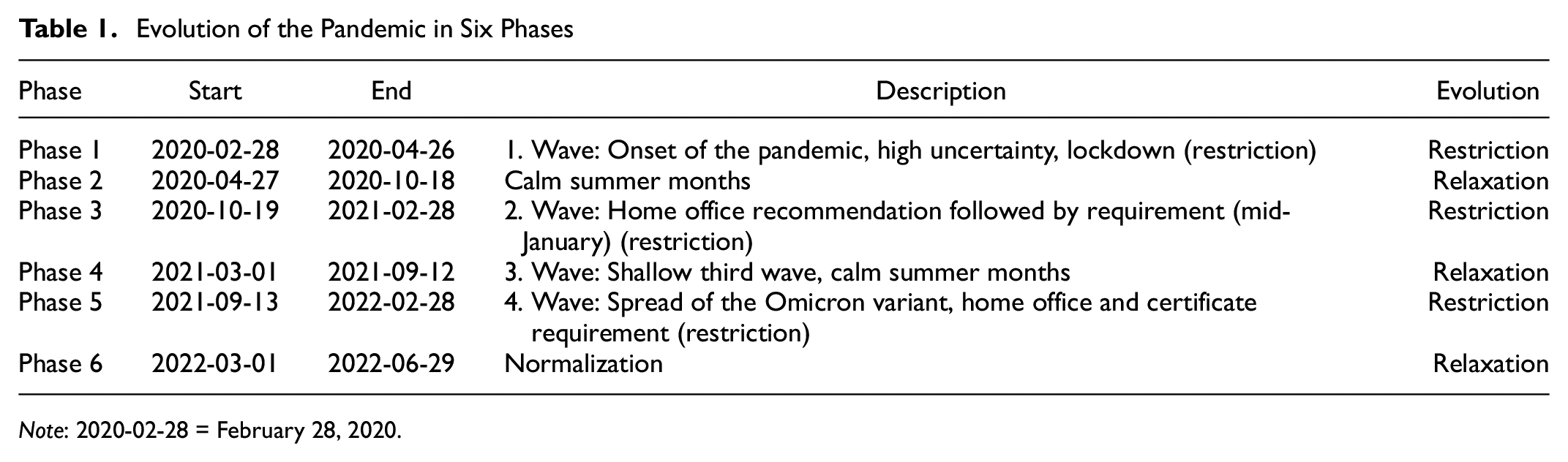
All the time-series graphs show moving averages (with a window size of 30 days) to filter the noise. For most figures, the evolution is depicted both in absolute numbers, comparing the average of the different phases (bar charts), and in relation to the baseline period, reflecting percentage deviations (line charts). Dotted vertical lines segment the time axis into the seven phases (each segment corresponding to one bar). Triangles mark end-of-September days which represent the midpoint of the baseline (and should therefore be comparable beyond seasonal patterns). Squares mark the end of the timeline, emphasizing the relative evolution since the beginning of the pandemic. The reader should keep in mind that the baseline is a rather arbitrary point in time (e.g., capturing the seasonal patterns of Switzerland’s autumn months) before the pandemic.
Not surprisingly, activity spaces, as measured by the 95% confidence ellipse area, were considerably depressed during the pandemic and are strongly governed by imposed COVID restrictions (see Figure 2). Seasonal patterns might exaggerate the effects of the pandemic, with prevalence being higher during winter months in which activity spaces usually are smaller. However, recent levels have not yet reached pre-pandemic ones. The home-office population reduced activity spaces more pronouncedly at the onset of the crisis but had slightly larger activity spaces compared with their work-outside-home peers in the calm summer months (phase 4). However, in the normalization phase, the activity spaces of the in-office population are again the largest. Therefore it is not clear whether home-office working depresses activity spaces in normal times. Further, considerable pre-pandemic differences in the levels exist: The participants working partly remotely and partly in-office had much larger activity ellipses in the baseline. Again, it is pivotal to understand that these people were not necessarily working in a mixed-working arrangement before the crisis, but were at the time of the survey. Nevertheless, this highlights how working arrangements segmented the population and affected transport demand by depressing the activity spaces of particularly mobile groups (with large activity spaces).
Change in activity spaces.
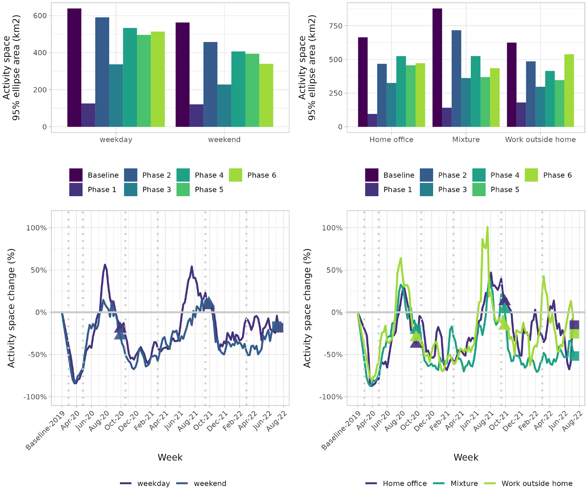
In Figure 3 the change in average daily distance as well as the change in number of stages by mode is depicted. A stage is a movement with one means of transport, including possible waiting times, in contrast to a trip, which is a sequence of stages from one activity to the next. All the modes react strongly to the evolution of the pandemic, with bicycle being the only mode that shows cyclical (correlated with case numbers) patterns and walking being relatively stable. PT (bus, train, tram) was considerably hit and has not yet recovered from the shift induced by the pandemic, with bus being the exception. Daily distance and number of stages show very similar patterns with similar magnitudes (percentage deviations). From Figures 2 and 3 together it could be argued that individuals tend to stay in closer proximity to their home location and therefore bicycle and bus are comparatively more frequently used (with the personal bicycle being available more freely).
Change in average daily distance and number of stages by mode.
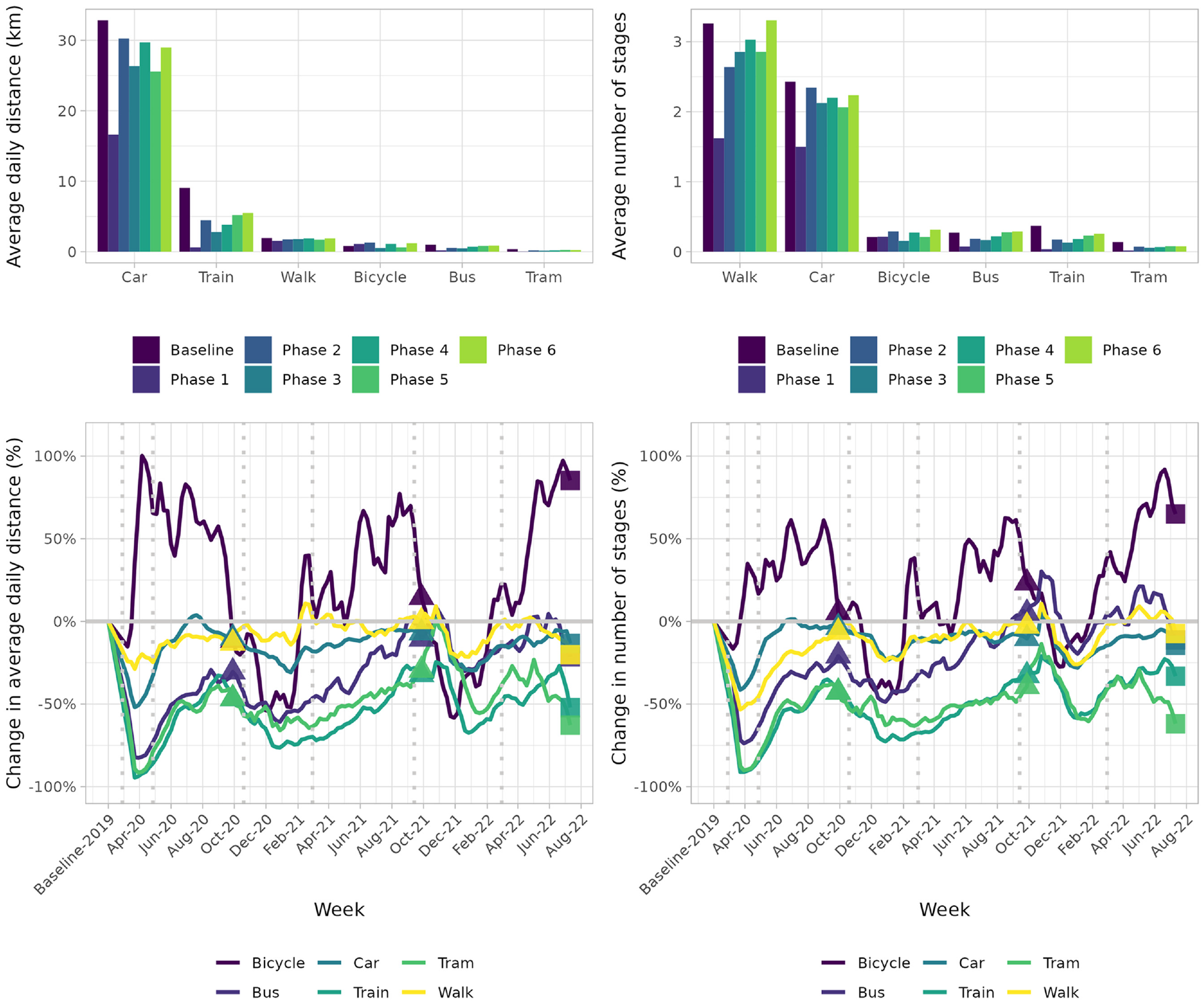
A very similar picture is portrayed in Figure 4 where we show average stage lengths and the average number of stages per day and by mode. The bicycle boom described by various authors (e.g., Molloy et al. [ 4 ] or Meister et al. [ 5 ]) has its foundation in the peak visible in the year 2020 and in bicycle being the only mode that benefited from restrictive measures. Despite bicycle stage lengths not reaching these very high levels, it is still the case that bicycle usage is slightly higher than during the pandemic. In particular, it is used more frequently. On the other hand, train travel has considerably reduced but is on a steady upward trend ever since. The reduction was primarily caused by fewer trips and not necessarily by shorter travel distances. One explanation could be that annual subscriptions (which reduce the marginal cost of PT travel considerably) got canceled in times of high uncertainty, making the mode less attractive, especially when accompanied by hygiene concerns.
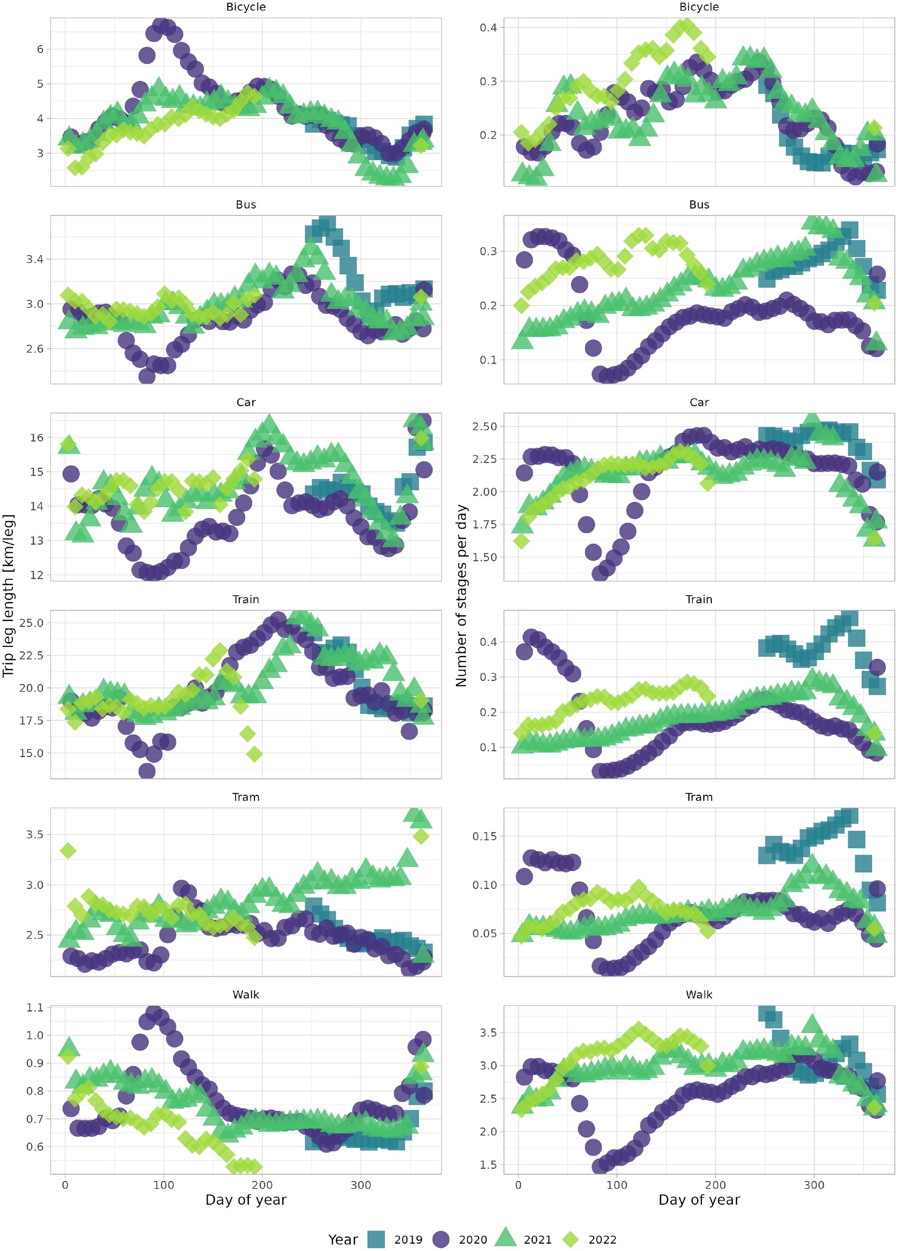
Average trip-leg length (left) and number of trips by mode (right). Comparison year on year.
Similarly, when differentiating by working arrangement, the collinearity between daily distances and number of stages is evident (see Figure 5). Both distances and number of stages could be reduced most pronouncedly by home-office working during the onset of the crisis. While the number of stages reached pre-pandemic levels for all working arrangements, daily distances did not for the more home-based peer groups. That is, the home-office population was more mobile before the crisis. Looking at absolute levels shows that people working at home during the crisis had a higher average daily distance in the baseline, potentially not because of the work situation but because of other moderating (socioeconomic) factors. Considering the latest phase, all working arrangements share similar levels. Therefore, one could again conclude, that home office does depress transport demand, not because the home-office population travel less per se but because they would have made particular long journeys in the absence of the hybrid working arrangement (e.g., long commuting distances which they now can avoid).
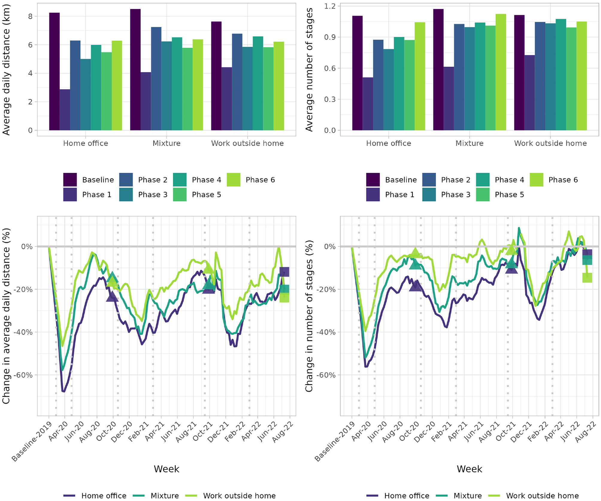
Change in average daily distance and number of stages by working arrangement.
Shifting attention to mode shares, Figure 6, we constructed two indicators: mode share based on how often a particular mode is chosen as the main mode (mode frequency) and mode share based on traveled distance. This reflects both the intensive (choice frequency) and extensive (covered distance) margin as well as the relative importance of the different modes. Bicycle has been able to expand its mode share along both dimensions (and beyond purely seasonal trends). Walking and car depict the most stable mode shares, with walking showing a pronounced peak in the distance share during phase 1 (as already noted in Figure 4). Interestingly, local PT has been affected differently: Bus has defended its mode share rigorously whereas tram has not been able to. Again, train steadily recovers from the big shock in phase 1 with a slightly higher recovery in its mode distance share. One explanation might be that people increased the number of short trips, where car and train are less likely to be considered.
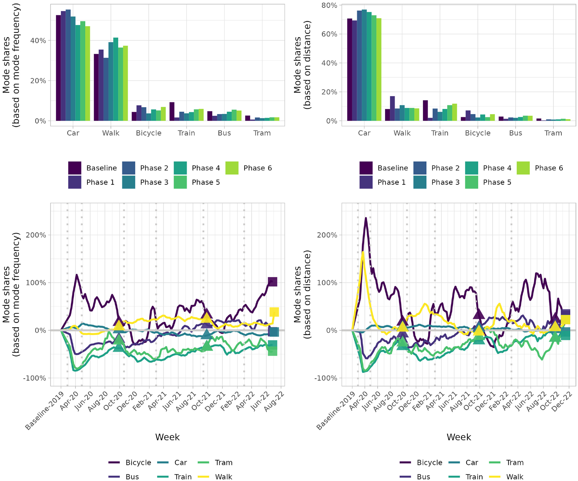
Mode shares by distance and mode choice frequency.
Figure 7 reveals the following insights: First, modal splits do not dramatically differ between the working arrangements. Second, train has lower mode distance shares across all working arrangements, which could be a result of ongoing hygiene concerns or a lagging recovery because of canceled subscriptions which are now so slowly renewed with decreasing uncertainty. Car increased its mode share only temporarily during the pandemic and the home-office population shows a slightly lower car distance share in phase 6 (compared with the other working arrangements). The walking boom during the onset of the pandemic can be attributed to the home-office population.
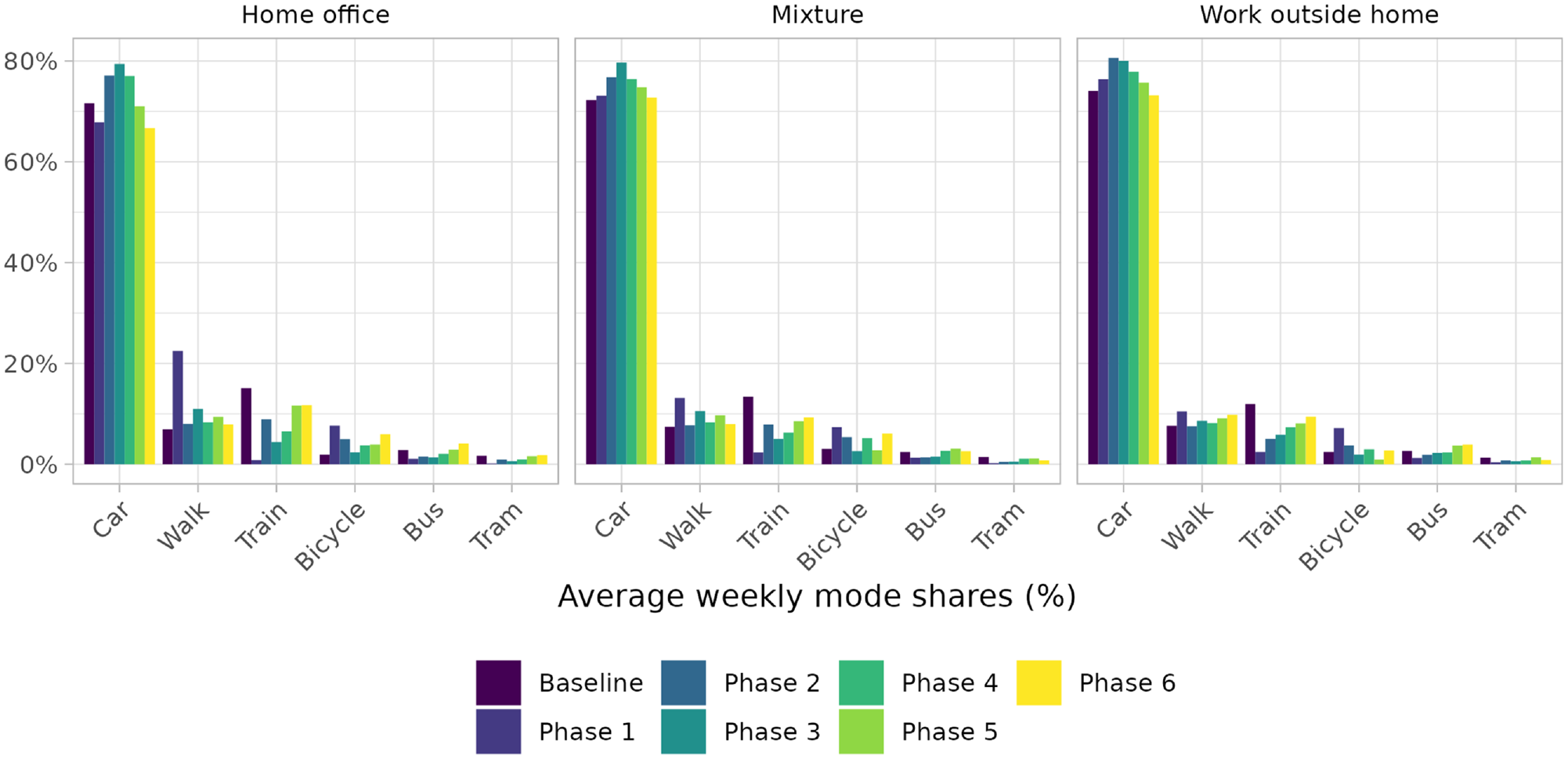
Mode distance shares by working arrangement.
Figure 8 shows the number of trips generated during a particular hour of the day and relative to the hour with the most trips (for each mode separately and differentiating weekdays and weekends as well as working arrangements). The left-hand side compares the data before COVID to the most recent values (after restrictions have been removed, that is, phase 6) while the right-hand side is based on phase 6 only.
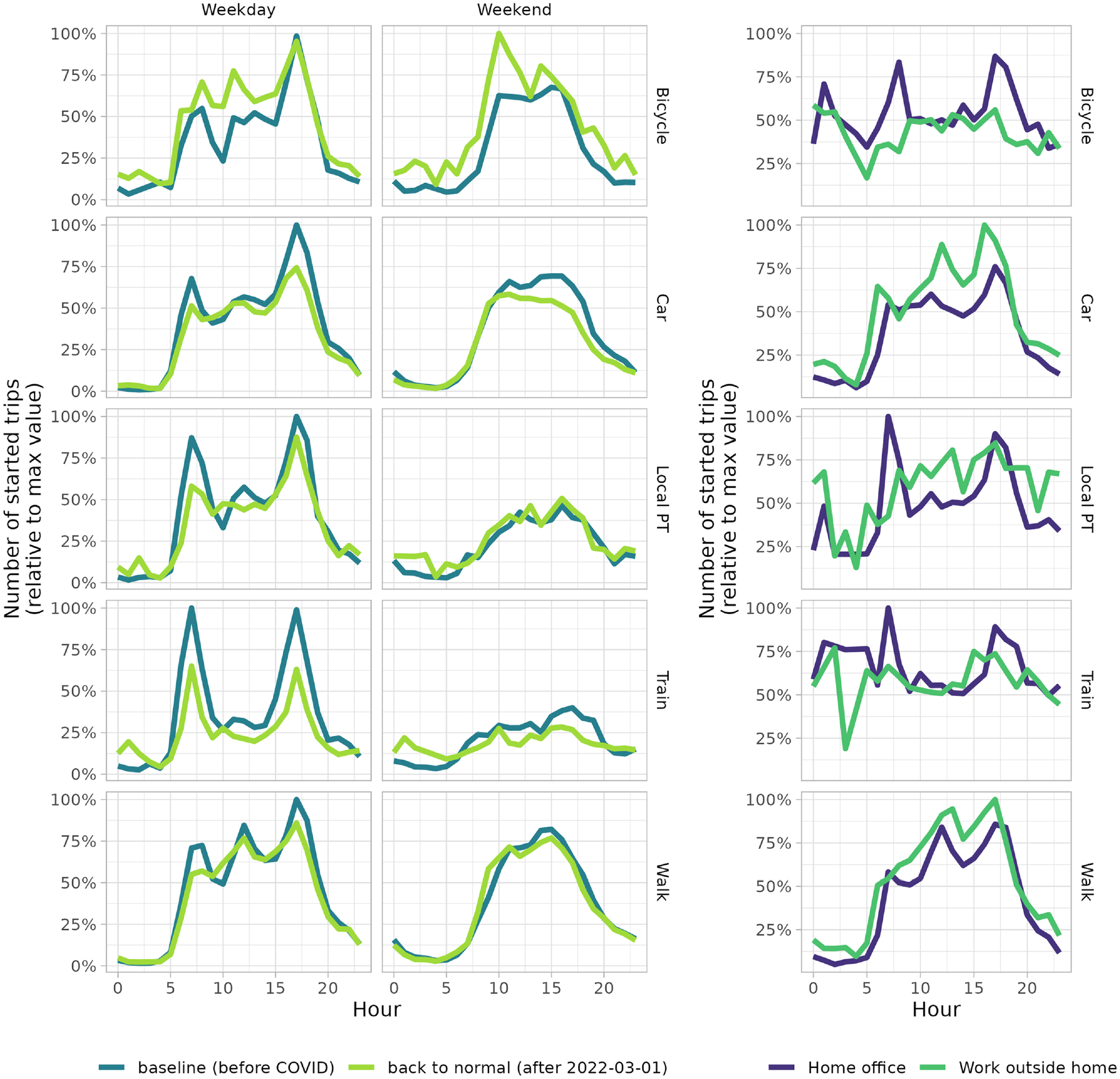
Hourly trip counts relative to busiest hour.
For example, looking at the train row and weekday column, most trips are generated during the morning and evening peak hours (which is the 100% reference hour) with the two peaks matching one another. Cycling increases during the day and at weekends (but not during commuting hours). Car and train show more or less a parallel downward shift. For train this shift is more pronounced than for car. The depression is less severe for local PT (bus and tram) than for train. For walk we see again the decrease during commuting peaks but otherwise, it is back to normal. Further, people working from home seem not to be that mobile during the day (most modes are almost identical during working hours, with bicycle being the exception). For car and train we see a decrease even during the weekend, which could imply either that people reduced activities or that they stayed in closer proximity to home (as local PT does not show this decrease, while bicycle increases…).
The pronounced morning and afternoon peaks of the home-office peer group for PT might reflect that if they work from the office space they choose PT—that is, the home-office population does not necessarily switch to car but has simply reduced its demand as a result of reduced commuting. On the other hand, we have seen that people working from home use more regional modes, in particular bicycle. The very similar trip generation of the home-office and the work-outside-home groups during working hours could again be interpreted as the home-office population not being that mobile during working hours.
The descriptive results are summarized below. Bicycle was the only mode used more intensively during restrictive phases. However, seasonal patterns could overemphasize this correlation. The bicycle boom was a temporary phenomenon that can be attributed to rather high stage lengths during the onset of the pandemic. Still, the bicycle is used more frequently in the normalization phase.
All PT modes (train, tram, bus) were considerably depressed by the pandemic. While train and tram have not yet fully recovered, bus has. Nevertheless, train has been on a steady upward trend ever since the initial shock.
Mode frequency shares decreased for car and train. This could be a consequence of people conducting more shorter trips where bus and bicycle have the advantage over car and train.
The impact of home office on activity spaces is ambiguous. During the pandemic, home office was an effective tool to reduce transport demand. In the normalization phase, average daily distances and average number of stages are almost identical among the three working arrangements. We hypothesize that home office depresses transport demand not because the home-office population travel less per se but because they would have made particular long journeys in the absence of the hybrid working arrangement (e.g., long commuting distances which they now can avoid). Modal splits do not dramatically differ between the working arrangements, with a slight preference for train for the home-office workforce. Car, on the other hand, is used less intensively.
MMDCEV Modeling Framework
In this section, the econometric framework is introduced. The multiple discrete-continuous extreme value model (MDCEV) was first formulated by Bhat ( 9 ). The model reflects on many consumer situations being characterized by multiple discreteness (a bundle of goods is consumed) of imperfect substitutes. In transportation, people choose both a portfolio of modes (discrete choice) and to what extent each mode is employed (continuous choice). Our formulation is derived from Meister et al. ( 5 ) and considers the two dimensions of mode choice (discrete) and choice of weekly distance shares by mode (continuous). The MDCEV models require a budget constraint and mode shares naturally add up to 1 which is the total budget a person can attribute to the available modes. Further, the marginal rate of substitution is constant (if you decrease the mode share of train by 1% you necessarily have to collectively increase the mode shares of the other modes by 1%) which abstracts from the cost component—that is, the budget line has slope 1. Such would not be the case if we were to model weekly mileage by mode.
The original model formulation incorporates both a translation parameter gamma (allowing for corner solutions) and a satiation parameter alpha (governing the marginal utility). However, it is well-known (e.g., Bhat [ 10 ]) that it is difficult to separate the two effects empirically (as the gamma parameter also has a satiation interpretation). Therefore, the modeler has to choose between three profiles (dropping or fixing one of the two parameters). We have estimated simple models with all the profiles and will from here onward only consider and present the so-called gamma-profile as it yielded the highest model fit.
In the following discussion of the panel MMDCEV (where the additional M stands mixed, i.e., in our case a random error component, introducing unobserved correlation between the two periods) model structure, individuals are indexed by

The term

where
It can be shown that conditional on the random error component, the probability of observing individual
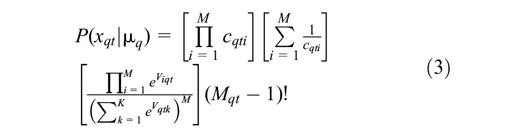
where

for
and

The parameters to be estimated are the

The unconditional likelihood can be formulated by marginalizing over the random vector

where

We used the Apollo package ( 11 ) and generated a Halton sequence of 1000 inter-individual draws to approximate the integral in Equation 7. Our model-building strategy included testing different profiles and different levels for the discrete variables as well as gradually increasing the model complexity and excluding insignificant variables. This process involved data of the normalization phase only. We further constructed variables reflecting on the mode-specific accessibility and a person’s living environment (e.g., degree of urbanization), and we controlled for weather characteristics. However, we carefully checked for collinearity and did not consider all the constructed variables (e.g., urbanization and access measures were closely related, as were temperature, humidity, and pressure levels).
Results and Discussion
We estimated the MMDCEV model based on the panel in the baseline and normalization (phase 6) periods, for which separate parameters were estimated except for
Model Estimates
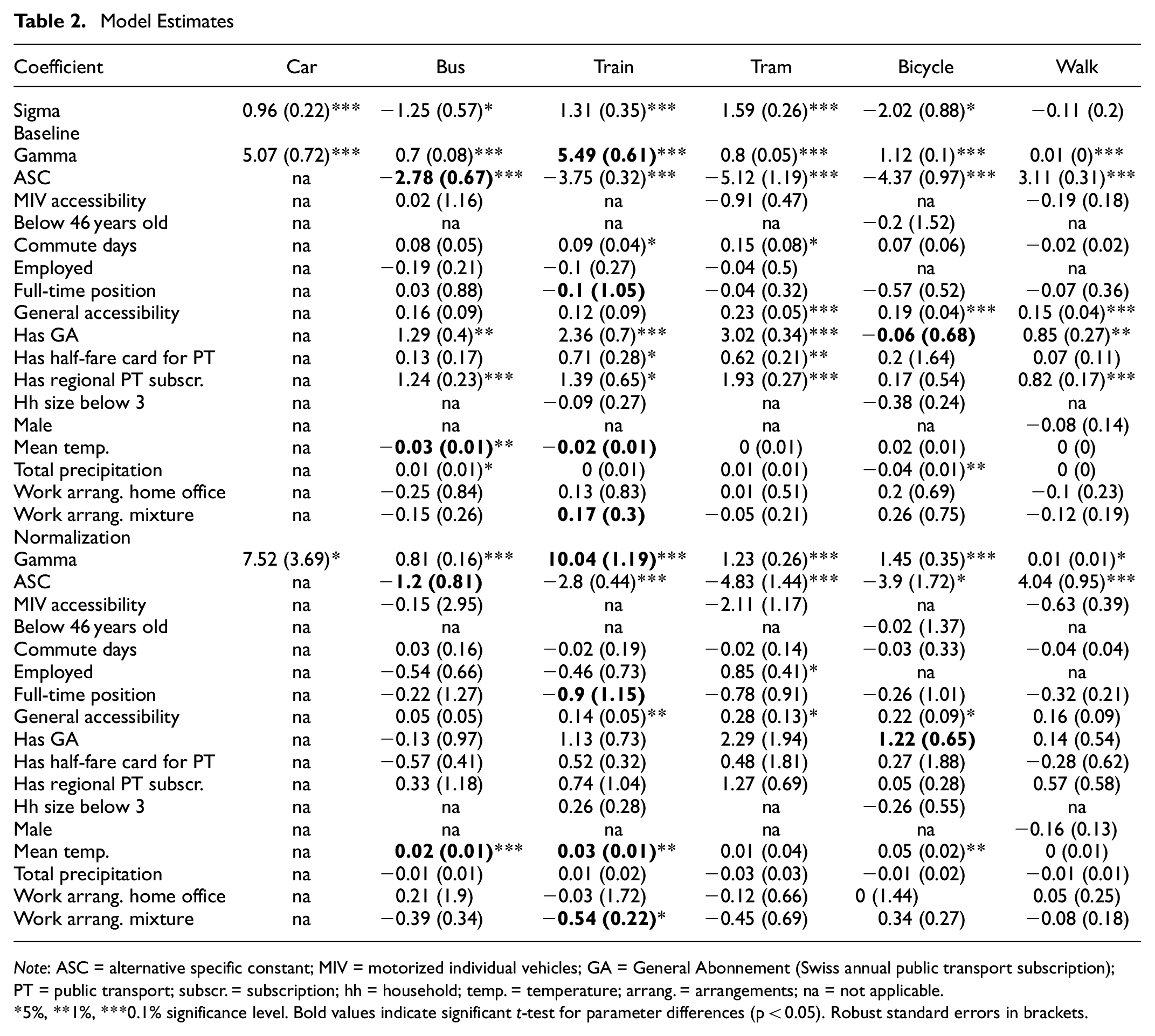
Note: ASC = alternative specific constant; MIV = motorized individual vehicles; GA = General Abonnement (Swiss annual public transport subscription); PT = public transport; subscr. = subscription; hh = household; temp. = temperature; arrang. = arrangements; na = not applicable.
5%, **1%, ***0.1% significance level. Bold values indicate significant t-test for parameter differences (p < 0.05). Robust standard errors in brackets.
Because of a smaller sample size in the normalization period, 95% confidence bounds are much wider. Therefore, while (considerable) differences between the two phases exist, most of these differences are not significant. It follows that there are no significant preference differences introduced by the pandemic. The remainder of the section should be read with this in mind. The notable exceptions include an increased ASC for bus, indicating that bus is chosen more frequently relative to car and compared with the baseline. Full-time employees choose the train less frequently which could imply that the pandemic induced a slight shift in commute modes away from train to car. Train’s satiation gamma on the other hand increased, which means that if train is chosen in a given week, its mode share tends to be considerably higher than before the pandemic. The workforce with a mixture work arrangement choose train significantly less frequently than before. Again, reduced commuting activity and a shift in commute mode could explain this. Finally, people with a GA (General Abonnement, a Swiss annual nationwide PT subscription) add a bicycle to their modal mix more frequently than before.
Considerable unobserved heterogeneity and panel effects are present at highly significant levels and across all modes except for walking (see sigma coefficient). Mode preferences are potentially governed by a wide array of personal attributes and attitudes which can be captured by the random error component.
As elaborated in the section on the MMDCEV modeling framework, the gamma parameter captures satiation and therefore the continuous mode-share dimension. Clearly, the parameter closely matches the observed patterns, whereby car and train have the highest mode distance shares by a wide margin. Interestingly, train is more satiated than car, which does not contradict observed patterns as gamma is conditional on having chosen the mode in a given week. That is, if train is chosen in a given week it tends to have a considerable mode distance share. Satiation increased across all modes from the baseline to the normalization phase, which can be read as individuals using the same modes more intensively.
Switching to the discrete dimension (where car is the reference alternative) all modes except for walk depict a negative average inter-individual utility (ASC). Interestingly, these differences diminished for all modes in the normalization period, indicating that the mode share of car lost ground relative to the other modes.
While the PT subscriptions (GA, Halbtax, and regional subscriptions) strongly predict PT usage in the baseline, they no longer do in the normalization. Potentially, a lot of the respondents canceled these subscriptions during the pandemic (and are still labeled as possessing these subscriptions whereas in reality, they do not).
Further, in line with the discussion of Figure 7, there are no significant differences in mode distance shares between the working arrangements (except for a decreasing train mode share for the mixture population, as previously discussed). This is to say, that there either are none or that differences are attributed to other socioeconomic factors or unobserved heterogeneity. In other words, working arrangements could segment the population along socioeconomic variables (such as education levels) which in turn potentially have different mode-share preferences. Also, modeling absolute mileage could prove more fruitful when eliciting differences between working arrangements.
In summary, individuals intensified the use of one particular mode as explained by increasing satiation parameters (however, only the difference in train satiation was significant). The car’s relative importance decreased with differences in ASC being positive. PT users canceled their subscriptions during the pandemic. Working arrangements do not predict mode-share preferences but could potentially still be an important lever as they could influence mode-share preferences via differences in socioeconomic characteristics. Future research should be devoted to understanding absolute differences such as mileage. The pandemic should not be read as a structural break in mode preferences as only a few parameters were found to differ between the two observation periods. This is in stark contrast to the study by Molloy et al. ( 4 ) and Meister et al. ( 5 ) who found considerable modal shifts induced by the pandemic. The findings from this work suggest that these changes were not made habitual but can be attributed to the unprecedented circumstances and constraints brought by the pandemic.
Conclusion and Outlook
This paper described the evolution of various mobility patterns before during and after the pandemic. The ambition was to understand modal splits and the impact of home office on transport demand beyond the COVID pandemic.
The key insights from our analysis are as follows: Both the bicycle and the walking boom were temporary phenomena. In the case of bicycle, exceptionally large stage lengths during the first phase explain the boom whereas for walking, the home-office population showed a pronounced peak during the first lockdown.
All PT modes were strongly depressed during the pandemic and car was able to temporarily expand its mode share. However, this was not a sustainable development and has normalized again. Bus was able to expand its mode distance share and train still shows a strong upward trend across working arrangements. With decreasing uncertainty and infection risk, further recovery of PT modes can be expected.
Mode frequency shares rebounded more strongly than distance shares. This could be explained by diminished commuting activity and shorter trips. Both factors could explain the attribution of mode share to bus and bicycle as these modes are more likely to be chosen on shorter stages.
It remains unclear to what extent and along which channels hybrid work arrangements affect transport demand. While home office was an effective tool for reducing transport demand during the crisis (and with enforced lockdowns) it is questionable whether these findings translate to normal times. Hybrid work arrangements segment the population along sociodemographic attributes and these segments have different mobility patterns. The MMDCEV model strengthens this hypothesis in so far as no significant preference differences can be attributed to the work arrangement attributes when controlling for sociodemographic factors (except for the mixture work and a negative coefficient for train). Therefore, modeling approaches that suggest no causal effect of home office on the variable of interest should keep in mind that the effect could be mediated over different user compositions.
While transport behavior was commented to be very different during the crisis, the pandemic should not be read as a structural break in mode preferences. This is probably also the most relevant policy implication of this paper: Changes observed during the pandemic (reduced peak traffic volumes, shifts to nonmotorized forms of transport and avoidance of PT) were not made habitual. Therefore pre-pandemic challenges translate to the post-pandemic era.
The presented analysis could be strengthened by estimating a panel MMDCEV on all stages simultaneously, similar to Meister et al. ( 5 ). The evolution of parameters throughout the pandemic could yield interesting insights. Further, more comprehensive post-estimation should be conducted, shifting focus onto variable leverage and sensitivity rather than significance (e.g., by computing marginal probability effects). Satiation parameters could be modeled as a function of socioeconomic attributes, shedding light on different satiation profiles. Further, it is essential to develop a better understanding of the home-office population to estimate the impact of new hybrid work arrangements on transport demand and beyond relative mode shares. Finally, model building and selection are said to be an art. The field could benefit from aligning its understanding of when it is justifiable to exclude non-significant variables as well as how to comment on the (absolute) quality of a model.
Footnotes
Acknowledgements
The authors would like to thank the three anonymous reviewers who took time to give quality feedback.
Author Contributions
The authors confirm contribution to the paper as follows: study conception and design: D. Heimgartner, K. W. Axhausen; data collection: D. Heimgartner; analysis and interpretation of results: D. Heimgartner; draft manuscript preparation: D. Heimgartner, K. W. Axhausen. All authors reviewed the results and approved the final version of the manuscript.
Declaration of Conflicting Interests
The author(s) declared no potential conflicts of interest with respect to the research, authorship, and/or publication of this article.
Funding
The author(s) disclosed receipt of the following financial support for the research, authorship, and/or publication of this article: The MOBIS-COVID data collection was financially supported by the Swiss National Railways (SBB) and the Kanton Zurich, and it received funding from the Swiss National Science Foundation and Innosuisse (Grant number 0820001327).
Data Accessibility Statement
The MOBIS-COVID data set can be shared for research purposes. Please contact the corresponding author daniel.heimgartner@ivt.baug.ethz.ch.