
Abstract
Autonomous vehicles (AVs) have moved from hype to reality as the penetration and acceptance rate continues to increase. As they are slowly integrated into traffic with human-driven vehicles (HDVs), it is necessary to predict the car-following behaviors of AVs and HDVs for better control of AV–HDV mixed traffic. This study extends a data-driven car-following model to incorporate drivers’ memory, and cooperation with the lead vehicle. The model predicts the following vehicle’s speed in AV–HDV mixed traffic. The effect of drivers’ cooperation on car-following behavior was modeled using prospect theory (PT), whereas the driver’s memory was incorporated using the memory cell of a long short-term memory (LSTM) neural network. This extended car-following model is called the “PT-LSTM model.” Real-world vehicle trajectories of HDVs and AVs in the Waymo AV Open Dataset were used to calibrate and validate the PT-LSTM model. The PT-LSTM model demonstrated higher accuracy compared with the LSTM model that did not consider drivers’ cooperation, the multiple layer perceptron model, Gipps’ model, and the intelligent driver model that incorporated PT. The importance of variables in different time steps in the PT-LSTM model was also evaluated using SHapley Additive exPlanations (SHAP). The SHAP results showed that AV followers were more likely to cooperate with the lead HDV, whereas HDV followers were more likely to cooperate with the lead AV than the lead HDV. Thus, this study underscores the importance of considering drivers’ memory and cooperation with the lead vehicle for the prediction of car-following behaviors in AV–HDV mixed traffic.
Autonomous vehicles (AVs) were developed to solve traffic problems such as traffic congestion, -safety, and -pollution. Although the penetration rate of AVs in traffic is still significantly low, it is predicted that AVs will become widespread in the years 2030 to 2040 ( 1 ). From this prediction, it is evident that it will take some time until all vehicles in traffic are AVs.
As more AVs are mixed with human-driven vehicles (HDVs), their interaction will be more frequent, and new car-following behaviors will be observed because of their different vehicle performance characteristics. Drivers’ car-following behavior generally depends on the lead vehicle’s motion, for example, drivers reduce speed if the lead vehicle decelerates ( 2 ). Thus, their car-following behavior is likely to vary with different types of lead vehicles (AV or HDV).
In an AV–HDV mixed-traffic scenario, there are four different groups of lead and following vehicle pairs: an AV following an AV (AV–AV), an AV following an HDV (AV–HDV), an HDV following an AV (HDV–AV), and an HDV following an HDV (HDV–HDV). HDV–HDV car-following behaviors have been widely studied in the literature. However, unlike HDV followers, who use driver perception to detect the lead vehicle’s motion, AV followers can better detect lead vehicle motion through sensors, and maintain shorter headways with the lead vehicle or reduce reaction times ( 3 ).
Interactions between HDVs and AVs have been modeled using separate mathematical car-following models for HDVs and AVs ( 4 ). However, in general, these models did not consider differences in car-following behavior among different types of lead and following vehicle pairs (HDV–AV, AV–HDV, and HDV–HDV). Moreover, models have generally been applied in microscopic traffic simulations, but they have not been calibrated and validated using real-world AV and HDV car-following data.
Thus, it was necessary to develop a model that could predict the car-following behaviors of HDVs and AVs that took into account their differences in vehicle performance characteristics and cooperation with the lead vehicle. In this study, cooperation between the lead and following vehicles was modeled using prospect theory (PT). The objectives of this study were as follows:
To analyze the car-following behaviors of HDVs and AVs for different types of lead and following vehicle pairs.
To model vehicle cooperation using PT and extend a data-driven car-following model to incorporate vehicle cooperation and driver memory (long short-term memory [LSTM] model) for predicting the car-following behaviors of HDVs and AVs.
The remainder of this paper is organized as follows: the next section reviews previous mathematical and data-driven car-following models applied in AV–HDV mixed traffic, AV-only traffic, and HDV-only traffic. The third section describes and analyzes real-world car-following data of HDVs and AVs. The fourth section describes PT, LSTM, and SHapley Additive exPlanations (SHAP), which determine the importance of variables in the model. The fifth section presents the results and discussion, and the final section summarizes the findings and makes recommendations.
Literature Review
Previous studies have developed mathematical models to predict car-following behavior. These classical car-following models are typically categorized on their underlying assumptions, the parameters they predict (such as spacing, acceleration, or speed), and the calibrated parameters. For instance, some models are classified as “collision-free” models, assuming that the following vehicle always maintains a safe distance from the lead vehicle to prevent rear-end collisions. Examples of such models are Gipps’ model ( 5 ), the intelligent driver model (IDM) ( 6 ), and the Krauss model ( 7 ).
On the other hand, there are stimulus-response models, like the General Motors model ( 8 ), which assume that the following vehicle reacts (accelerates or decelerates) based on the motion of the lead vehicle. Some models are also categorized as psychophysical models because they consider the perception and reaction times of the driver, such as the Wiedemann model ( 9 ). These established models have laid the foundation for understanding car-following behavior, however, they do not consider all the factors that can affect this. As a result, researchers have extended and refined these models to improve their performance. For instance, the models incorporate other factors, such as honking effects, backward-looking effects, and other contextual factors ( 10 – 14 ). It is worth noting that these conventional models have mainly focused on HDVs following HDVs.
Some researchers have developed car-following models where the lead and following vehicles are AVs. For example, Friji et al. developed a car-following model using a reinforcement learning neural network and high dimensional red green blue depth frames ( 15 ). Xoap et al. proposed a car-following model for AVs that assumes that the behavior of the following vehicle is affected by two or more preceding vehicles ( 16 ). They found the model could achieve optimal microscopic and macroscopic performance compared with other models such as the IDM. Sharma et al. developed an extended IDM for connected vehicles that incorporated driver compliance with information ( 17 ). The driving strategy developed using PT was used for calibrating this. Sharma et al. found that the extended IDM better predicted car-following behavior than the original.
Some researchers have developed data-driven car-following models that can replace mathematical models. For instance, Shi et al. developed a data-driven car-following model using random forest, and showed that the model could better predict car-following behavior than the GM model ( 18 ). Hao et al. developed a data-driven car-following model based on rough set theory ( 19 ), and Zhang et al. developed a model based on genetic algorithms ( 20 ). Other data-driven models, which outperformed mathematical methods, have been put forward ( 21 – 25 ). Data-driven car-following models that consider the effect of driver memory have also been proposed ( 26 – 31 ). These models utilize recurrent neural networks (RNNs), gated recurrent units, or LSTM models to replicate human driving styles, and have demonstrated promising results in capturing complex car-following behaviors.
The aforementioned studies primarily focused on AV–AV or HDV–HDV behavior in car-following models, neglecting AV–HDV and HDV–AV interactions. To address this gap, some researchers have developed more comprehensive car-following models for mixed-traffic environments involving both AVs and HDVs. For example, Cao et al. proposed a generic car-following model for both AVs and HDVs in mixed traffic flow while considering different market penetration rates of AV ( 32 ). The model utilized an improved IDM encompassing driver memory for HDVs, and an extended cooperative adaptive cruise control (CACC) car-following model based on a nonlinear dynamic headway for AVs. The proposed model was shown to effectively model car-following behavior under different market penetration rates of AVs. Liu et al. proposed an extended IDM that can capture the car-following behavior of AVs under a heterogeneous platoon by assuming a 35% market penetration rate for AVs ( 33 ). The proposed model considered the effect of the preceding connected vehicles within the communication range of the following AV. The proposed model was found to be more stable than traditional IDMs. Rahmati et al. carried out an experimental study to investigate the difference between HDV–HDV and HDV–AV interactions in mixed traffic ( 34 ). They found that human drivers felt more comfortable and showed risk-taking behavior when they followed AVs. Stabler et al. ( 35 ) and Ahmed et al. ( 36 ) modeled HDV–AV interactions using dynamic traffic assignment models and car-following models in microscopic traffic simulation, respectively. Ding et al. also developed an extended IDM for AVs and HDVs that incorporated cooperation between drivers, modeled using PT ( 37 ) . Unlike other studies that made use of simulated data, they used the field data observed from three Tesla vehicles in mixed traffic flow. The results indicated that the model captured the heterogeneity of car-following behaviors in AV–HDV mixed traffic.
Zhu et al. simulated car-following behavior in mixed traffic flow using a multiagent system ( 38 ). The reliability of the simulation was tested using the data collected from actual roads. The multiagent simulation showed that mixed HDV and AV traffic will move at a faster speed and with smaller between-car spacing. Zhu and Zhang proposed a car-following model for AVs in AV–HDV mixed traffic with adjustable sensitivity and smoothing factors. They verified the correctness of the proposed car-following model using numerical simulation ( 39 ). Ozkan and Ma studied car-following behavior and energy efficiency in AV–HDV mixed traffic using inverse reinforcement learning ( 40 ). The model had the capacity to learn and replicate the observed car-following behavior. The study also showed that HDVs consume less fuel when following AVs. Using a driving simulator, Schoenmaker et al. investigated the car-following behavior of HDVs when following AVs ( 41 ). They found that HDV drivers maintained a significantly shorter time headway when driving in the proximity of AV platoons. Lin et al. developed an LSTM model that considered Connected and Autonomous Vehicles (CAVs) following AVs using the NGSIM (i.e., Next Generation Simulation) dataset ( 42 ). They tested the attention-based LSTM model at different market penetration rates and found that the model provided more accurate longitudinal trajectory predictions for different time steps. Wen et al. investigated the interactions between HDVs and AVs using time-to-collision, driving volatility measures, and principal component analysis using the Waymo Open Dataset ( 43 ). They identified that HDV–AV traffic exhibited lower driving volatility compared with HDV–HDV.
In summary, the aforementioned studies have certain limitations, such as the use of simulated datasets that do not accurately represent real-world vehicle trajectories, and the utilization of mathematical models that may not fully capture complex driver behaviors. Thus, this study aimed to overcome these limitations by extending a data-driven car-following model to incorporate driver cooperation with the lead vehicle using PT, and driver memory using LSTM. The model was calibrated and validated using real-world vehicle trajectory data from AVs and HDVs. By combining PT with LSTM, we were able to account for the effects of driver (or AV) memory and cooperation with the lead vehicle on car-following behavior. To the best of our knowledge, this is the first study to incorporate PT into LSTM for predicting car-following behavior in AV–HDV mixed traffic.
Methods and Data
This section is divided into three subsections: first, a description of the data and analysis of car-following behavior in AV–HDV mixed traffic using real-world vehicle trajectory data; following this, PT for modeling cooperation; and finally, LSTM for the prediction of car-following behavior.
Data and Analysis
The real-world vehicle trajectory data used in this study were obtained from Waymo LLC, a leading AV technology company. The data were collected from multiple cities across the United States including San Francisco, CA, Phoenix, AZ, and Mountain View, CA ( 44 ). The data were collected using Lidar and camera technologies, capturing vehicle trajectories from diverse road segments such as freeways and urban streets. This was carried out at different times of the day, encompassing various weather conditions to ensure a comprehensive representation of real-world driving scenarios.
For each vehicle, the data were collected at a time interval of 0.1 s. The data included the type of vehicle (HDV or AV); speed (in m/s); road segment; weather condition; time of day; and the length, width, and height of the vehicle; acceleration; position (x and y coordinates); spacing between the following and lead vehicle; and the ID of the lead vehicle. The data provided trajectory data spanning a total of 300,000 s, which allowed a comprehensive analysis of car-following behavior.
Specifically, the data included 1,032 vehicle pairs for HDV–HDV, 274 vehicle pairs for HDV–AV, and 196 vehicle pairs for AV–HDV. The data did not include trajectories for AV–AV vehicle pairs. As a result, the analysis in this study was limited to three groups of vehicle pairs: HDV–HDV, HDV–AV, and AV–HDV. Despite this limitation, the data still provided valuable insights into car-following behavior in AV–HDV mixed-traffic scenarios and meaningful analysis and findings.
To ensure the highest level of data accuracy and reliability, a curated, preprocessed version of the Waymo dataset was provided by Hu et al. for this study ( 44 ). Given its size, this dataset served as a robust foundation for investigating the interactions and behaviors of diverse vehicle types in mixed-traffic scenarios.
The dataset was initially checked for noise and irregularities to ensure data quality. To achieve this, a Savitzky-Golay (SVG) filtering algorithm was applied to the global positioning data (x and y coordinates) of all vehicles in the original dataset. The SVG filtering algorithm is commonly used for smoothing time series data owing to its ability to filter out noise in a series of equally spaced data values by applying a polynomial fit. For instance, Figure 1 provides a comparison between the smoothed position and the original position of two randomly selected vehicle trajectories. The similarity between these positions indicated that the original dataset had minimal noise. Next, the output of the SVG filtering algorithm was used to calculate the speed of each vehicle in the dataset. The speed was calculated using Equation 1 as follows:

where
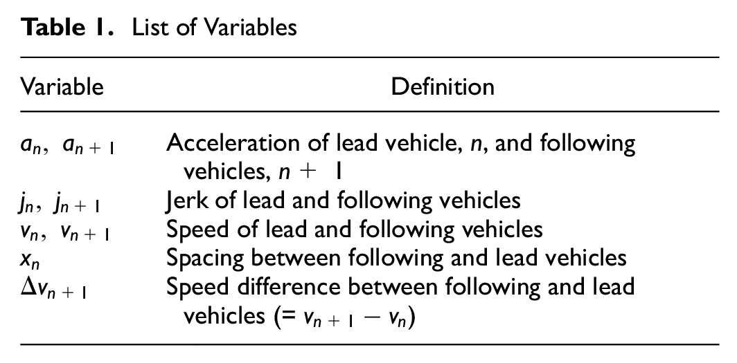
The car-following behavior for all three types of vehicle pair was analyzed using eight of the core variables in the original dataset, as shown in Table 1.
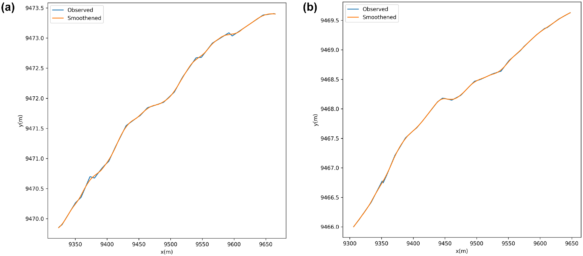
Comparison of original and smoothed vehicle positions: (a) Vehicle 1 and (b) Vehicle 2.
List of Variables
Initially, a safety critical analysis was conducted for each type of vehicle pair, taking into consideration different ranges of spacing. The distribution of acceleration for different ranges of spacing is depicted in Figure 2. The analysis revealed that when the spacing between vehicles was greater than 15 m, the behavior was similar for all three vehicle pair groups. However, when the spacing was less than 15 m, the acceleration of an AV following an HDV tended to concentrate more around zero compared with the acceleration of an HDV following an AV or HDV following another HDV. This observation suggests that AVs tended to maintain a more consistent speed to ensure a safe distance from the lead vehicle compared with HDVs.
Distribution of a following vehicle’s acceleration for different ranges of spacing: (a) spacing 10 m, (b) 10
A comparison of spacing distributions was also conducted among the three vehicle pair groups, as illustrated in Figure 3. The analysis revealed that the median and variance of spacing were similar between HDV–AV and AV–HDV vehicle pairs. However, the median spacing was smaller for HDV–HDV pairs. Furthermore, the figure also indicated that the median spacing for HDV–HDV pairs was slightly longer than the median spacing for HDV–AV pairs. This observation implies that the car-following behavior of HDV drivers may vary depending on the type of lead vehicle (AV or HDV), indicating that human drivers may adjust their following distance differently based on the type of vehicle they are following.
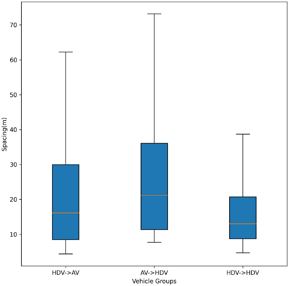
Distribution of spacing for different vehicle pair groups.
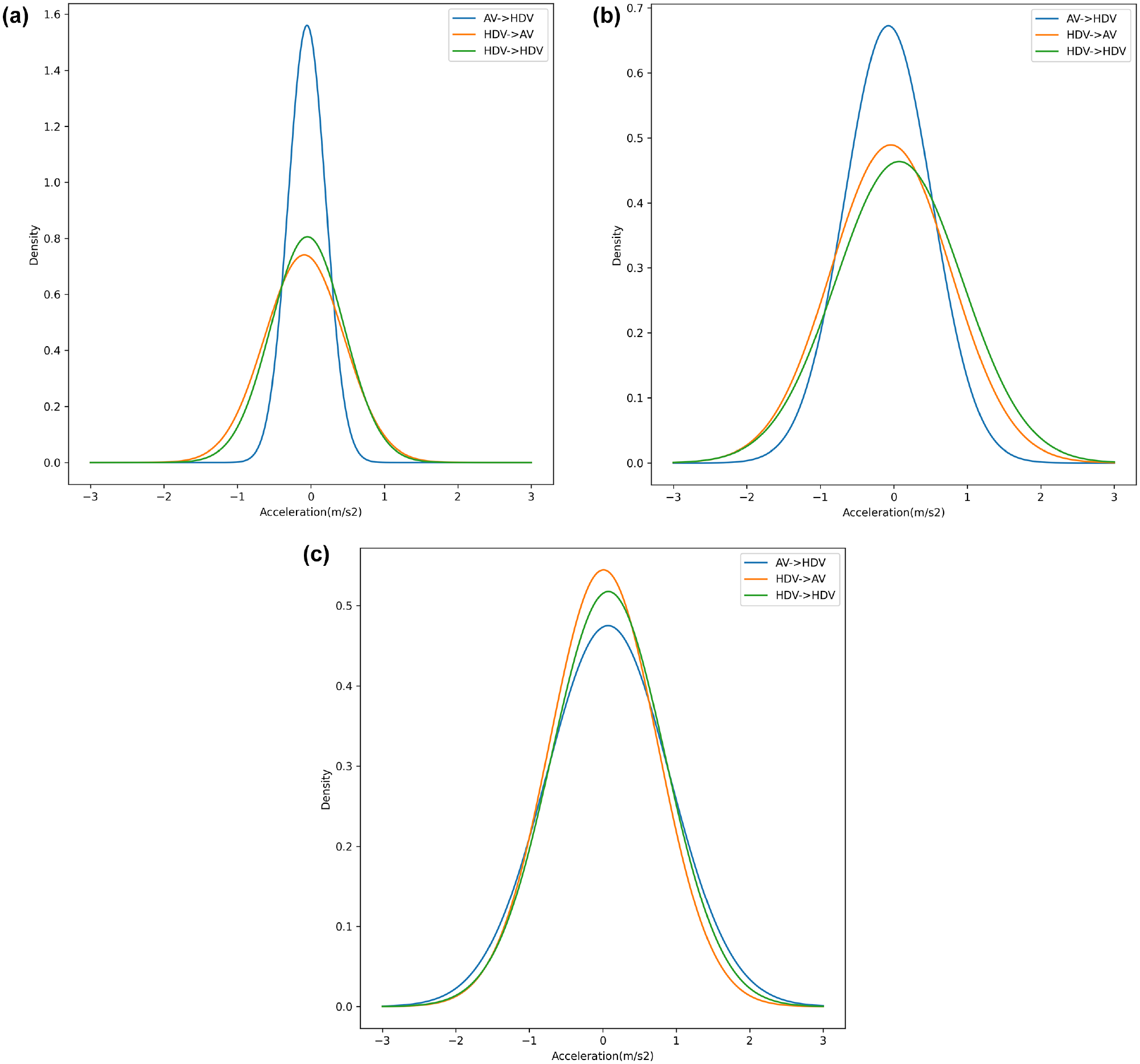
Figures 4 and 5 display the distribution of acceleration and jerk of the following vehicle, respectively, in relation to the spacing for the three vehicle pair groups. Jerk represents the rate at which the acceleration of either the following vehicle or the lead vehicle changes. Figure 4 reveals that when an HDV followed an AV, the deceleration tended to be more concentrated in the 10- to 30-m range of spacing. However, when an AV followed an HDV, deceleration and acceleration were concentrated on small values close to zero within a low ≤10-m range of spacing. A similar trend was observed for spacing ranges ≥35 m. Furthermore, Figure 5 shows that the distribution of jerk followed a similar pattern to that of speed. These results suggest that AVs were capable of better speed control without the need for hard deceleration compared with HDVs when following another vehicle.
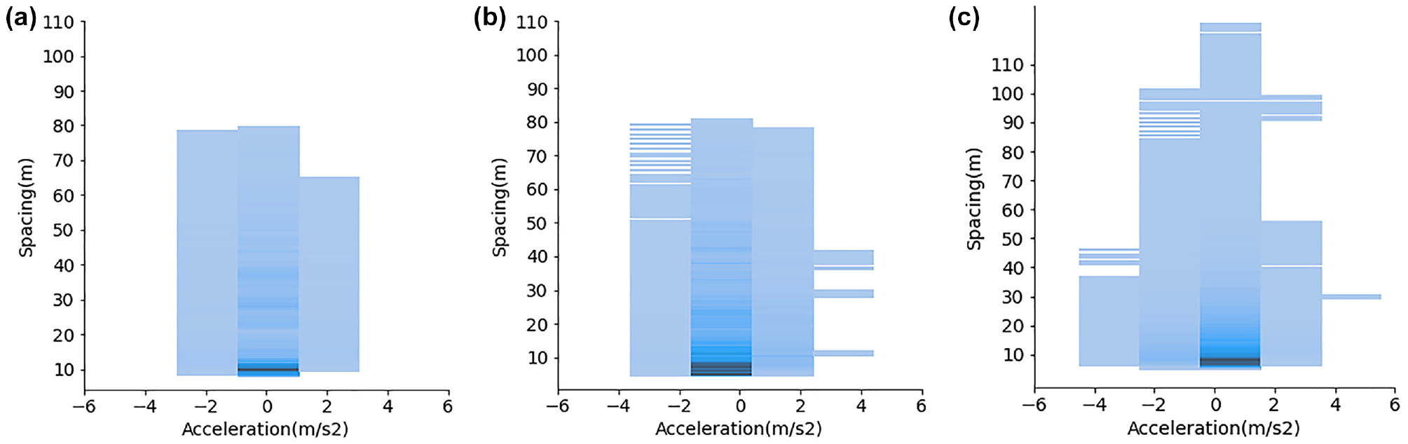
Distribution of acceleration for different vehicle pair groups: (a) AV following HDV, (b) HDV following AV, and (c) HDV following HDV.
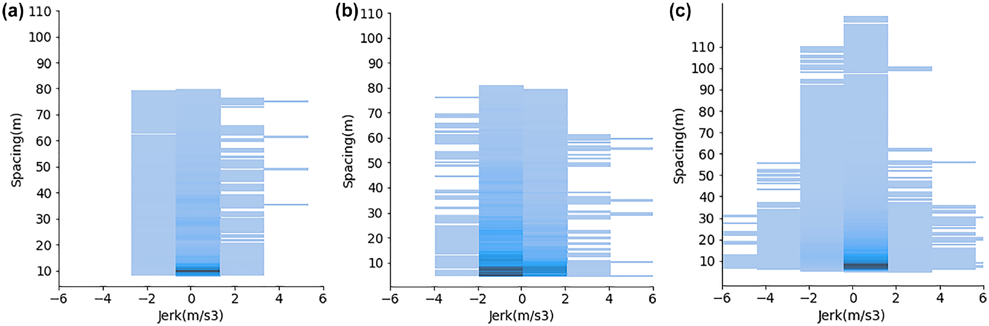
Distribution of jerk for different vehicle pair groups: (a) AV following HDV, (b) HDV following AV, and (c) HDV following HDV.
Figure 6 shows the distributions of spacing and velocity difference between the following and lead vehicles. The figure reveals that the distributions were similar between HDV–AV and HDV–HDV vehicle pair groups. However, for the AV–HDV pair group, the velocity difference was relatively smaller at larger spacing ranges of 10 to 48 m. This suggests that AVs tend to maintain smaller velocity differences with HDVs at larger spacing ranges compared with HDV–AV and HDV–HDV pairs. A smaller velocity difference may indicate that AVs are better able to maintain safe and consistent spacing.
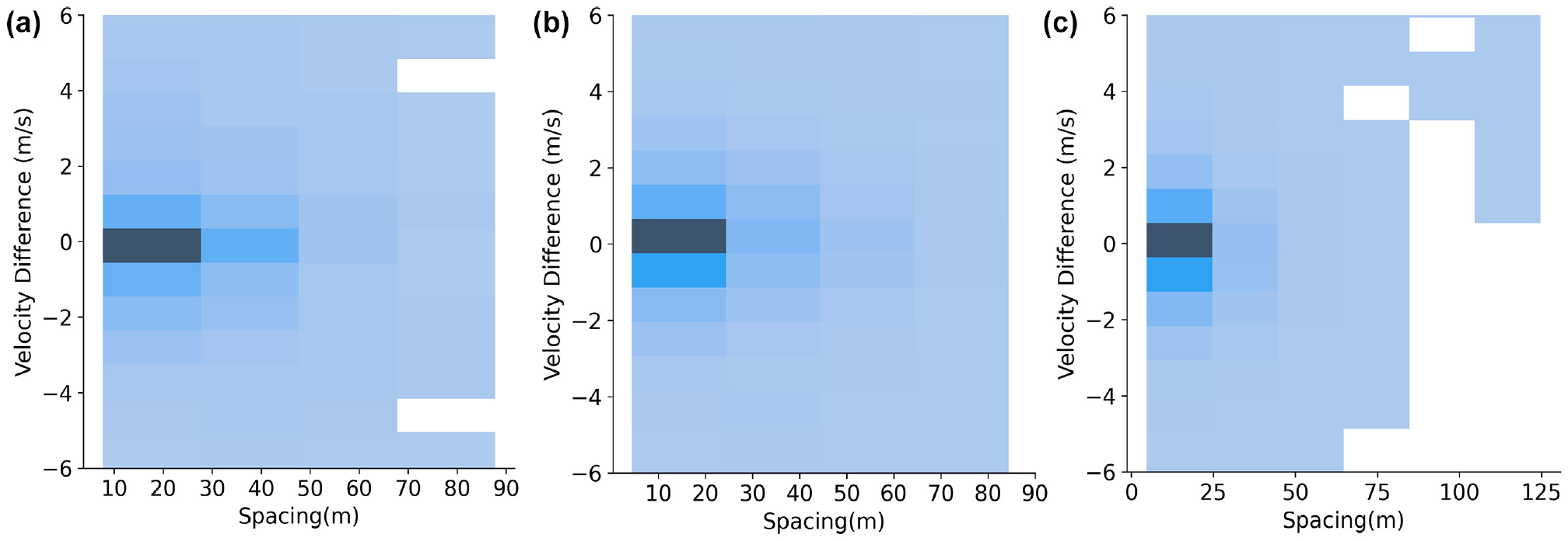
Distribution of velocity difference for different vehicle pair groups: (a) AV following HDV, (b) HDV following AV, and (c) HDV following HDV.
Lastly, the mutual information (MI) algorithm was adopted to investigate the relationships between selected variables and the velocity of the following vehicle at the next time step,
Figure 7 displays the ranking of MI shared between the selected variables and the velocity at the next time step. The results revealed that the ranking of the variables for HDV–AV and HDV–HDV pairs was similar. However, when an AV was following an HDV, the spacing with the lead vehicle and the lead vehicle speed exhibited almost equal potential in reducing uncertainty with the velocity of the following vehicle at the next time step. This finding aligned with expectations, as AVs utilize sensor data to simultaneously control maneuvers based on the observed lead vehicle’s speed and spacing, making them more adaptive in mixed-traffic scenarios.
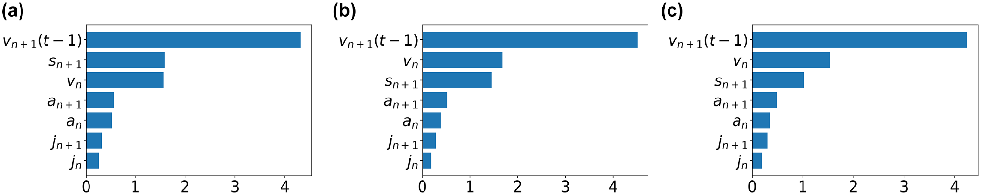
Mutual information ranking for different vehicle pair groups: (a) AV following HDV, (b) HDV following AV, and (c) HDV following HDV.
Prospect Theory for Modeling Cooperation
PT has found application in various domains, such as mental accounting in behavioral economics and modeling driver compliance or route choice in transportation ( 46 ). PT was introduced by Kahneman and Tversky, who observed that risk decisions are often influenced by subjective considerations that, in turn, may have been shaped by language expressions, leading to different preferences in different scenarios ( 47 ). In the context of a car-following model, PT can be used to show that drivers may not always make decisions based solely on rational calculations of expected outcomes. Instead, they may evaluate potential gains and losses in a subjective and biased manner, taking into account factors such as the perceived risk of collision, comfort level, and potential benefits of following closely. PT also proposes that individuals are more sensitive to losses than gains, resulting in risk-seeking behavior in certain situations. Incorporating these behavioral aspects in car-following models can enhance their ability to capture the subjective decision-making processes of drivers in real-world traffic scenarios.
In PT, the decision makers’ choices are first formulated through prospects and then the utility value of each prospect is calculated (
37
). The prospect value,

where

where

where
The PT curve generated through the utility function,
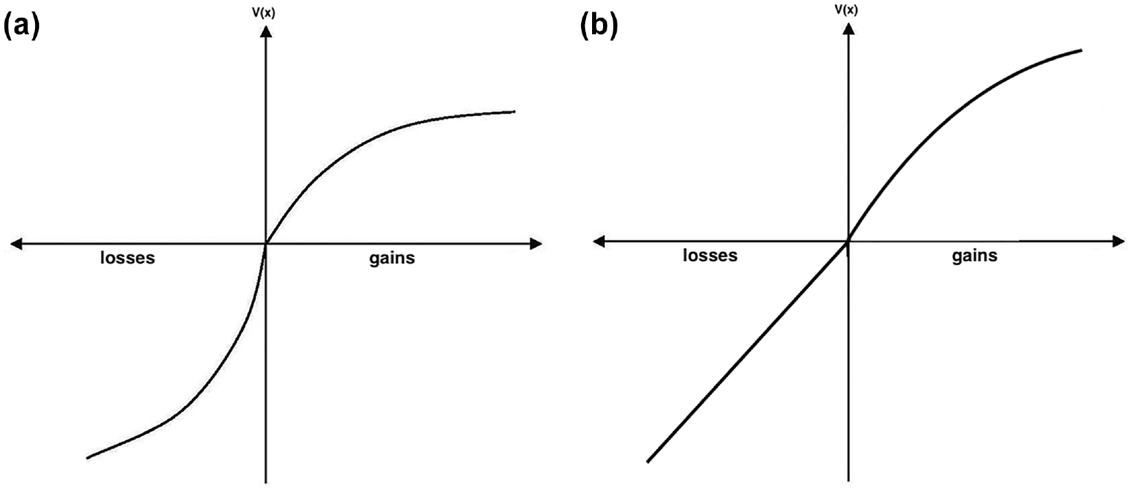
Prospect theory curves: (a) α≤ 1 and (b) λ > 1 ( 37 ).
However, if
In an AV–HDV mixed-traffic environment, AVs and HDVs have different car-following behaviors and vehicles may have different preferences that lead to different response regimes to the same situation in surrounding traffic conditions. In this study, the cooperation between vehicles in car-following conditions was modeled using PT based on the spacing with the lead vehicle, as proposed by Ding et al. ( 37 ). The cooperation value was measured with a range of 0 to 1. A cooperation value close to zero means a lower likelihood of change in the car-following behavior in response to the lead vehicle’s speed and represents low cooperation. On the other hand, a cooperation value close to 1 means a significant change in the car-following behavior and represents high cooperation. It was expected that as the spacing increased, the cooperation value would decrease and vice versa. The cooperation function is represented as follows ( 37 ):

where
As the urgency value,

where
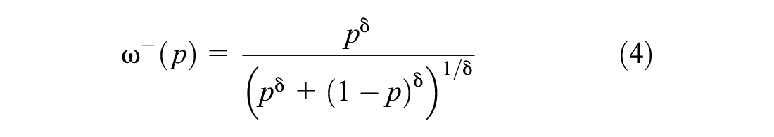
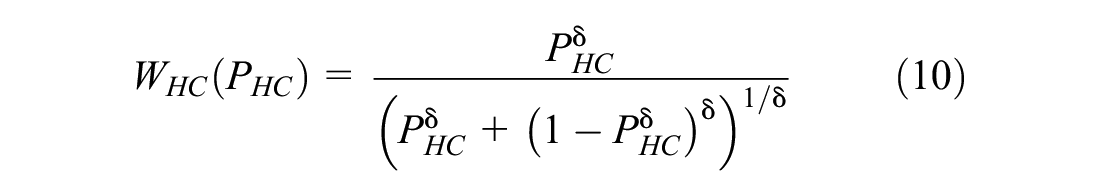
Similar to PT, the weighting function for gains and loss is represented as the weighting function for low cooperation, WLC, and high cooperation, WHC,

where

As the observed spacing approaches the spacing at
where

As the observed spacing approaches the spacing at

where


In this study, PT was used to model the perceived gains and losses when the following vehicle was uncertain of the lead vehicle’s future behavior. The output from PT, the cooperation utility,
Long Short-Term Memory Neural Network
An LSTM neural network (NN) is a specific type of RNN with a longer memory and better transition ability. The network is best known for its ability to effectively solve sequential problems such as speech recognition, image recognition, and time series problems owing to its ability to store previously encountered patterns in its memory for the prediction of future patterns.
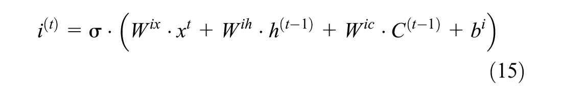
Similar to typical NNs, the LSTM-NN has three layers: the input layer, the hidden layer and the output layer. The input layer is the first layer in the network and it initializes the input variables for the subsequent layers. The output layer is responsible for giving the output. The hidden layer is the most important feature of LSTM-NN because it has memory cells that consist of gates to solve vanishing gradient problems as it passes information from one sequence to another ( 29 ). This feature allows LSTM-NN to learn long-term relationships between complex features in a dataset. Through these memory gates, which are capable of updating, discarding, and retaining information, LSTM is able to mimic the human decision-making process. The LSTM gates are divided into three types:
Input gate: Takes the independent variables as input into the network and decides which new information should be stored.

Forget gate: Determines which part of the processed information of the previous output state should be retained in the knowledge base.
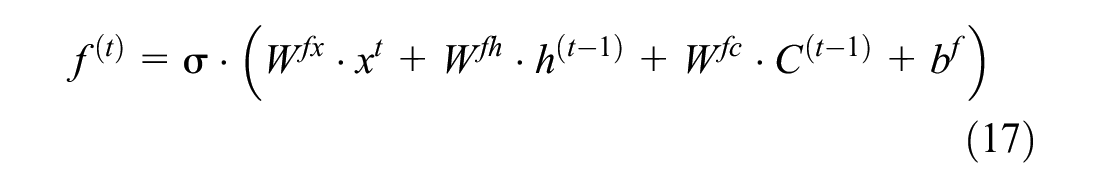
Output gate: Transfers the processed data as an input to the input gate of the hidden layer at the next time step.
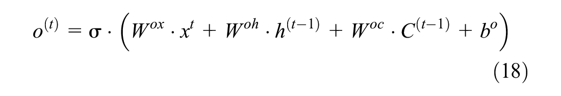
where


The LSTM-NN is then trained to reduce the loss function, which evaluates how well the network fits the data. The most popular loss function is mean squared error (MSE) as follows:

where
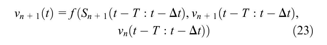
Based on the results of the MI (Figure 7) and the cooperation utility of PT, the LSTM model predicts the following vehicle’s speed in the current time step,
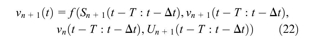
where
In this study, the memory attribute of LSTM was used to model the driver’s memory in car-following behavior. This study considered two different models: the LSTM model that incorporates PT to consider the cooperation utility—the “PT-LSTM model” (Equation 22); and the LSTM model that does not consider the cooperation utility—the “baseline LSTM model” (Equation 23) as follows:
SHAP for Determining Importance of Variables of Models
Understanding why a complex machine learning model makes a certain prediction has become an important part of many scientific applications. In this regard, SHAP has been applied as an interpretable machine learning framework, similar to the permutation importance (PIMP) that helps interpret model predictions and underlying properties of data. Unlike the PIMP, which measures variable importance based on how a feature affects model performance, SHAP measures the importance of a feature based on the magnitude of attributions. SHAP function was derived from game theory and was developed on the additive feature attribution method that unifies six feature importance methods ( 48 ). This approach allows SHAP to be less affected by highly correlated values, unlike PIMP. The SHAP function is described as follows:
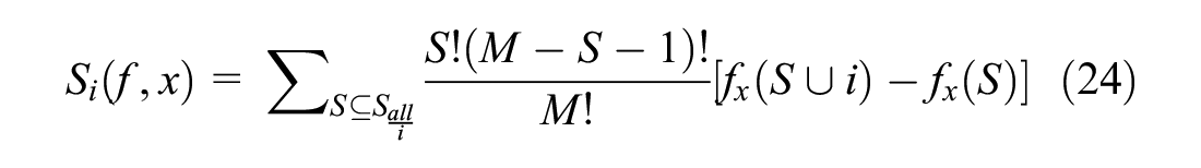
where
Although SHAP produces more accurate results than PIMP and other variable importance methods, it is computationally intensive. This means that when the number of input features (N) is large, the computational complexity becomes 2 N , which is very expensive ( 49 ).
Results and Discussion
The PT-LSTM model and the baseline LSTM model were estimated using Python on Google Colab owing to the availability of more processing power. To ensure that there was no overfitting, cross-validation using TimeSeriesSplit was implemented where KFold was set to 3 at all times and 20% of the data were used for testing. For each KFold, 20% was used for validation and 60% for training. First, the baseline LSTM model was estimated. Table 2 shows the LSTM configuration parameters that gave the lowest root mean square error (RMSE) after performing an informal search. It is worth noting that this might not be the optimal value.
LSTM Configuration Parameters
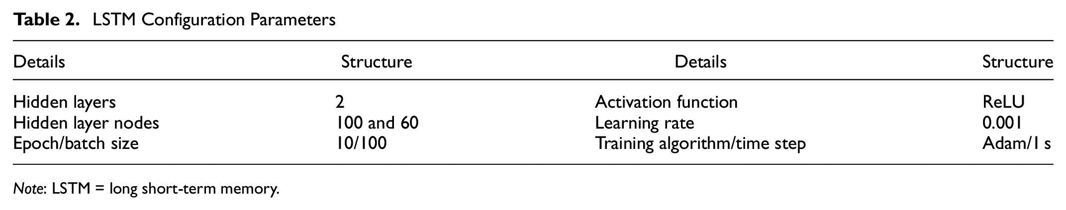
Note: LSTM = long short-term memory.
After estimating the baseline LSTM model, the PT-LSTM model was estimated using the LSTM configuration parameters in Table 2. The PT parameter for each vehicle pair group of HDV–AV, HDV–HDV, and AV–HDV was calibrated separately using differential evolution (DE) and the optimization function that gave the lowest RMSE was derived. Each parameter of the DE function was set as follows: the population size, the maximum number of generations, and the function tolerance were set to 100, 300, and 1e−6, respectively. Table 3 shows the range of each parameter value used while calibrating PT parameters for each vehicle pair group using DE.
Range of Parameter Values in Prospect Theory
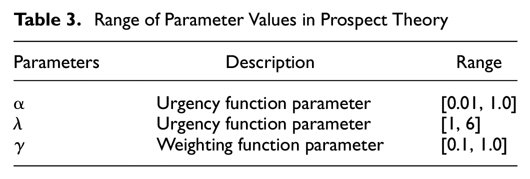
Table 4 presents the RMSE for different sets of the PT parameters. The table shows 10 randomly selected DE-calibrated outputs including the baseline LSTM model and the PT-LSTM models with RMSE values. The first result on the list is the RMSE of the baseline LSTM model. The parameters in bold are from the PT-LSTM model with calibrated PT parameters that produced the lowest RMSE. The table shows that the RMSE of the PT-LSTM model with the lowest RMSE was lower than the RMSE of the baseline LSTM model. This result indicates that the LSTM model with the cooperation utility (PT-LSTM model) outperformed the baseline LSTM model.
Calibration of Cooperation Utility Parameter Values with LSTM
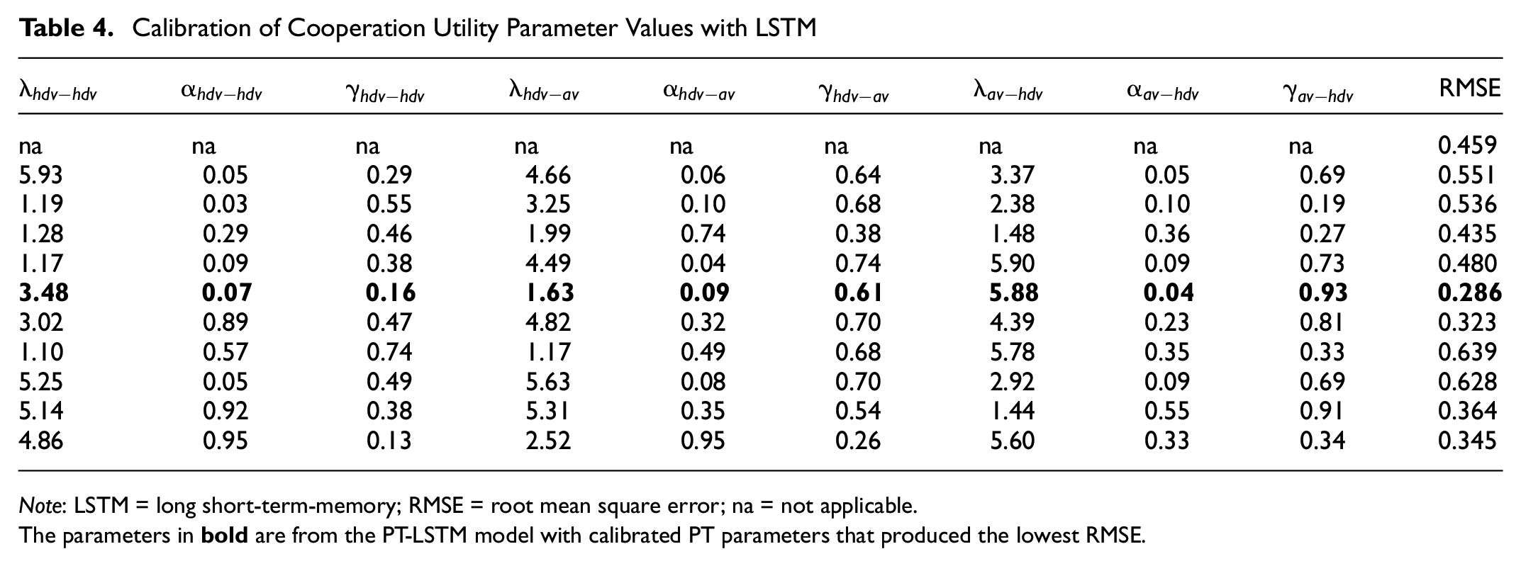
Note: LSTM = long short-term-memory; RMSE = root mean square error; na = not applicable.
The parameters in
From Table 4, it can be seen that the
The distributions of the urgency value,
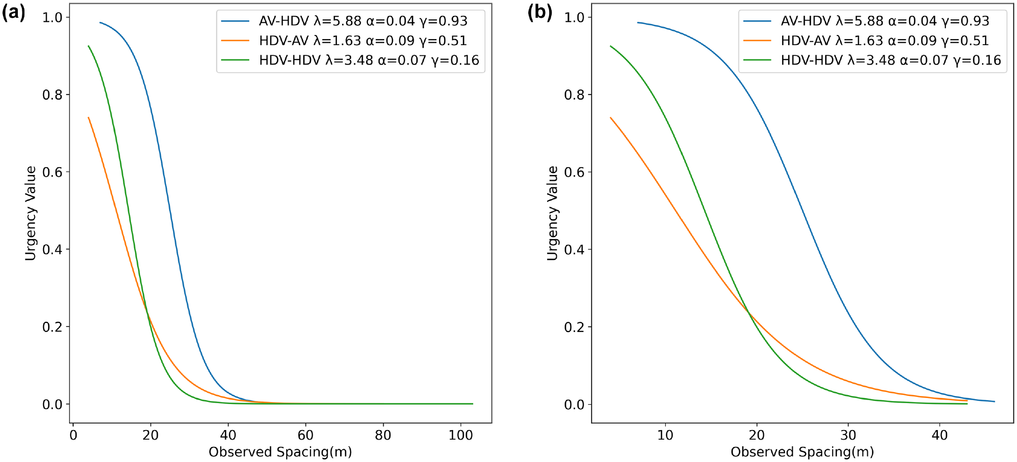
Urgency value of the LSTM with calibrated parameters: (a) urgency value and (b) urgency value (spacing of 0 to 50 m).
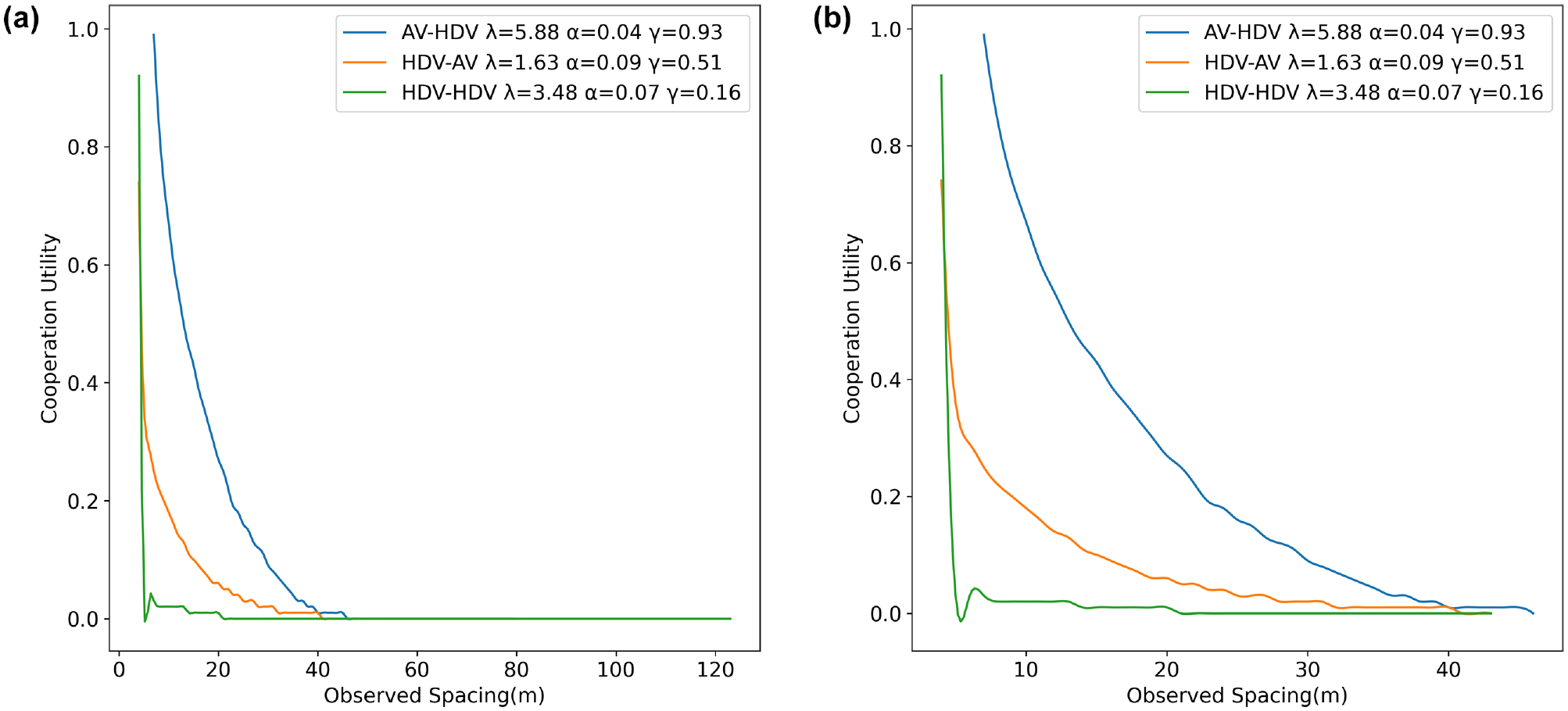
Cooperation utility value of the LSTM with calibrated parameters: (a) cooperation plot based on U value and (b) cooperation plot based on U value (spacing of 0 to 50 m).
Figure 10 shows that the cooperation utility values were lower for HDV followers than AV followers for a given spacing. This result indicates that HDVs were more aggressive in their car-following behavior (i.e., they were less likely to cooperate with the lead vehicle unless the spacing was very short) regardless of the lead vehicle type. However, AVs are able to track and cooperate with the lead vehicle through sensors in a car-following environment. It is also important to note from the figure that the cooperation utility increased more slowly as the spacing decreased for HDV–AV than HDV–HDV pairs. This suggests that HDVs had a more prolonged level of cooperation with the lead AV than when following the lead HDV. This HDV–AV behavior can be attributed to the longitudinal velocity control mechanism of AVs ( 43 ).
Figure 11 presents a comparison of prediction accuracy for the following vehicle speed among the PT-LSTM model, baseline LSTM model, and a time-series-based multiple layer perceptron (MLP) model for each vehicle pair group. The results demonstrate that the PT-LSTM model achieved lower RMSE than both the baseline LSTM model and MLP model for all vehicle pair groups. Specifically, the difference in RMSE between the PT-LSTM model and the baseline LSTM model was more pronounced for HDV–AV than for AV–HDV and HDV–HDV. Therefore, the PT-LSTM model outperformed both the baseline LSTM and MLP models, demonstrating greater accuracy in predicting the interaction between an HDV and an AV in mixed traffic.
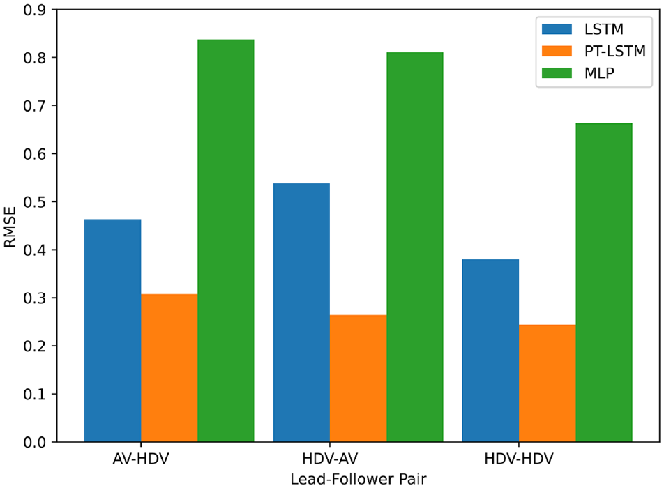
Comparison of prediction accuracy between models for each group of vehicle pair.
We further adopted SHAP to compare the importance of variables in the PT-LSTM model. Figure 12, a to c , shows the SHAP output for AV–HDV, HDV–AV, and HDV–HDV, respectively. A higher SHAP value indicates the greater import a variable has to the prediction of car-following behavior. The figure shows that the following vehicle speed and the lead vehicle speed at previous time steps were most important for the prediction of the following vehicle speed in the current time step.
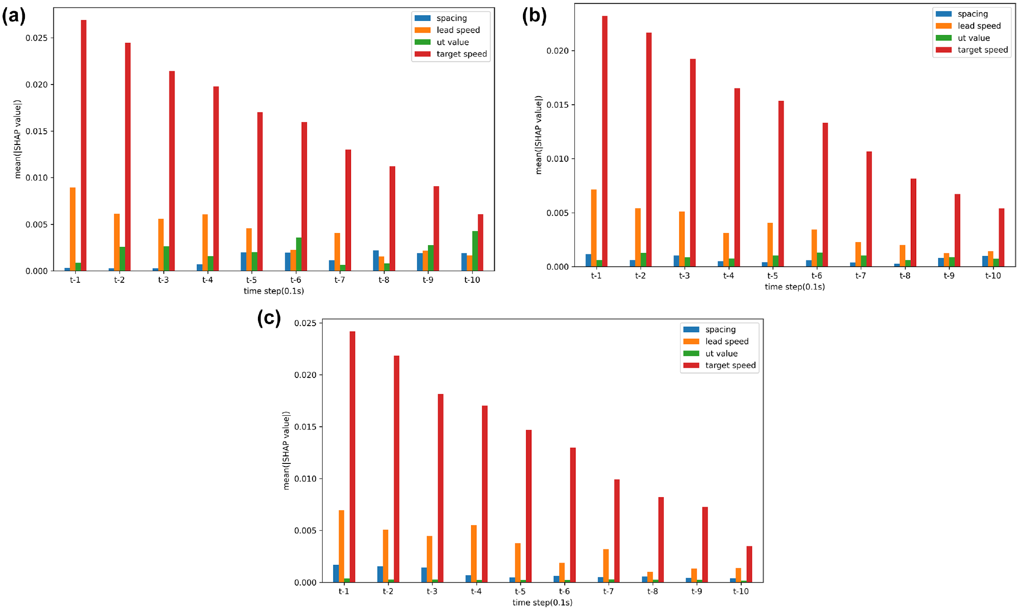
Importance of variables of PT-LSTM model determined using SHAP: (a) AV following HDV, (b) HDV following AV, and (c) HDV following HDV.
Moreover, the SHAP value of the cooperation utility (ut value) was relatively higher for AV–HDV than HDV–AV and HDV–HDV. This result suggests that AVs following HDVs are more likely to control their behaviors based on the cooperation utility, unlike HDV drivers following AVs or HDVs. This is because the following AV is more likely to cooperate with the lead HDV. However, for HDV–HDV, the SHAP value was consistently higher for spacing than the cooperation utility in all time steps, and its cooperation utility was lower than AV–HDV and HDV–AV. This means that HDV drivers following HDVs were more likely to control their behaviors based on the spacing and less likely to cooperate with the lead HDV. Also, the SHAP value of the cooperation utility was slightly higher for HDV–AV than HDV–HDV. This indicates that HDV drivers were more likely to cooperate with the lead AV than the lead HDV. This is intuitive because HDV drivers generally have a greater level of comfort and trust when they follow an AV than an HDV ( 50 ).
The PT-LSTM model was compared against two other car-following models, namely the PT-IDM (IDM with the incorporation of PT) proposed by Ding et al. ( 37 ), and Gipps’ model, which is widely recognized as a collision avoidance model. The PT-IDM is described as follows:
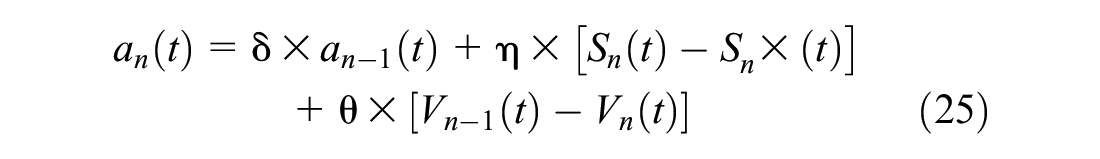

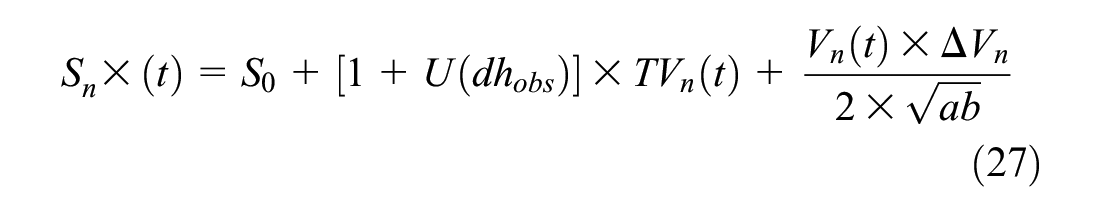
where
S
n
(t) and
δ, η, and θ are parameters to be calibrated.
To compare the PT-IDM, Gipps’, and PT-LSTM models, a total of six vehicle pairs were carefully selected, with two pairs chosen for each vehicle group. To fine-tune the parameters of the PT-IDM and Gipps’ models, the DE optimization technique was used with a population size of 100, a maximum number of 300 generations, and a function tolerance of 1e-6. For the PT-IDM, the parameter ranges for S0, a, b, T, δ, η, and θ were set to [2, 10], [0.1, 5], [0.1, 5], [0.1, 5], [0.1, 5], [0.1, 5], and [0.1, 5], respectively, whereas the PT parameters λ, α, and γ were fine-tuned using DE with the ranges set to [0.01, 0.5], [1, 6], and [0.1, 1], respectively. For Gipps’ model, parameter ranges for
Tables 5 and 6 display the optimal calibration parameter set used for each vehicle pair. Figure 13 shows the comparison of vehicle speeds, including observed speed, and predicted speed by PT-LSTM, PT-IDM, and Gipps’ model. The findings revealed that the PT-LSTM model outperformed the PT-IDM and Gipps’ model in relation to accuracy in predicting the observed following vehicle speed for all three vehicle pair groups.
Calibration of Parameter Values of PT-IDM with Cooperation Utility
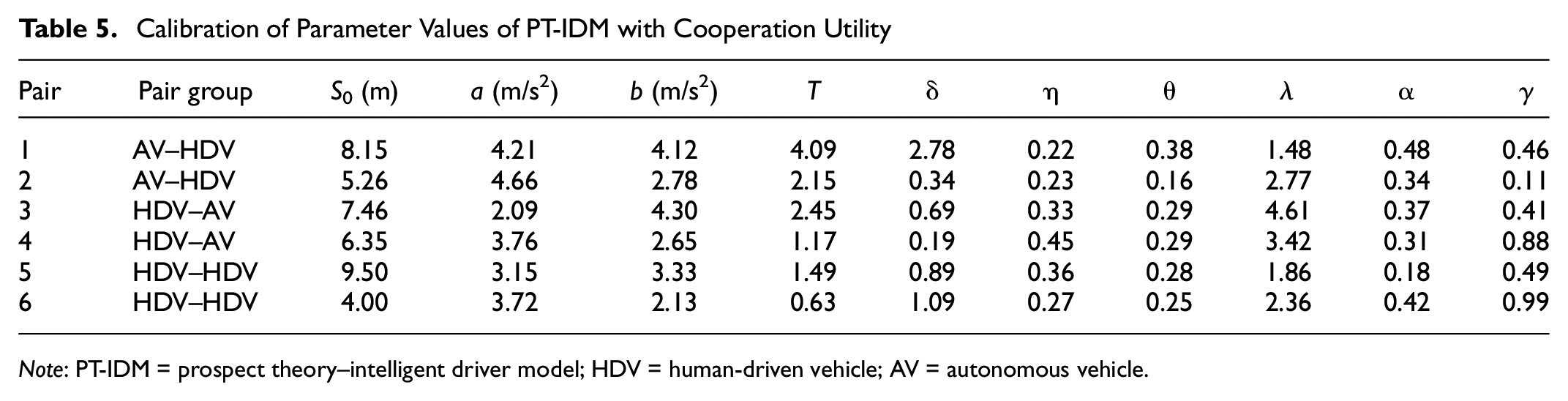
Note: PT-IDM = prospect theory–intelligent driver model; HDV = human-driven vehicle; AV = autonomous vehicle.
Calibration of Parameter Values of Gipps’ Model
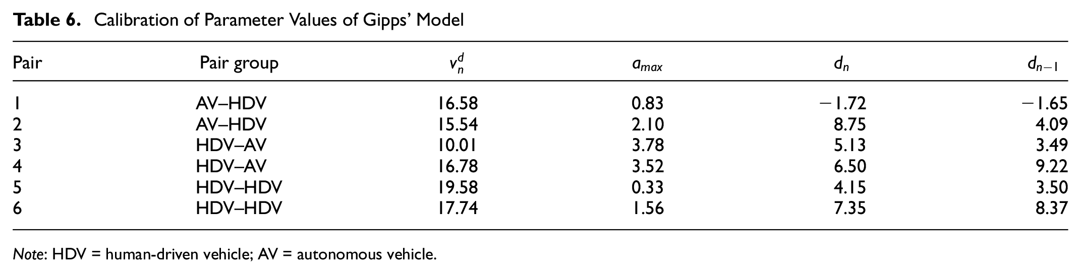
Note: HDV = human-driven vehicle; AV = autonomous vehicle.
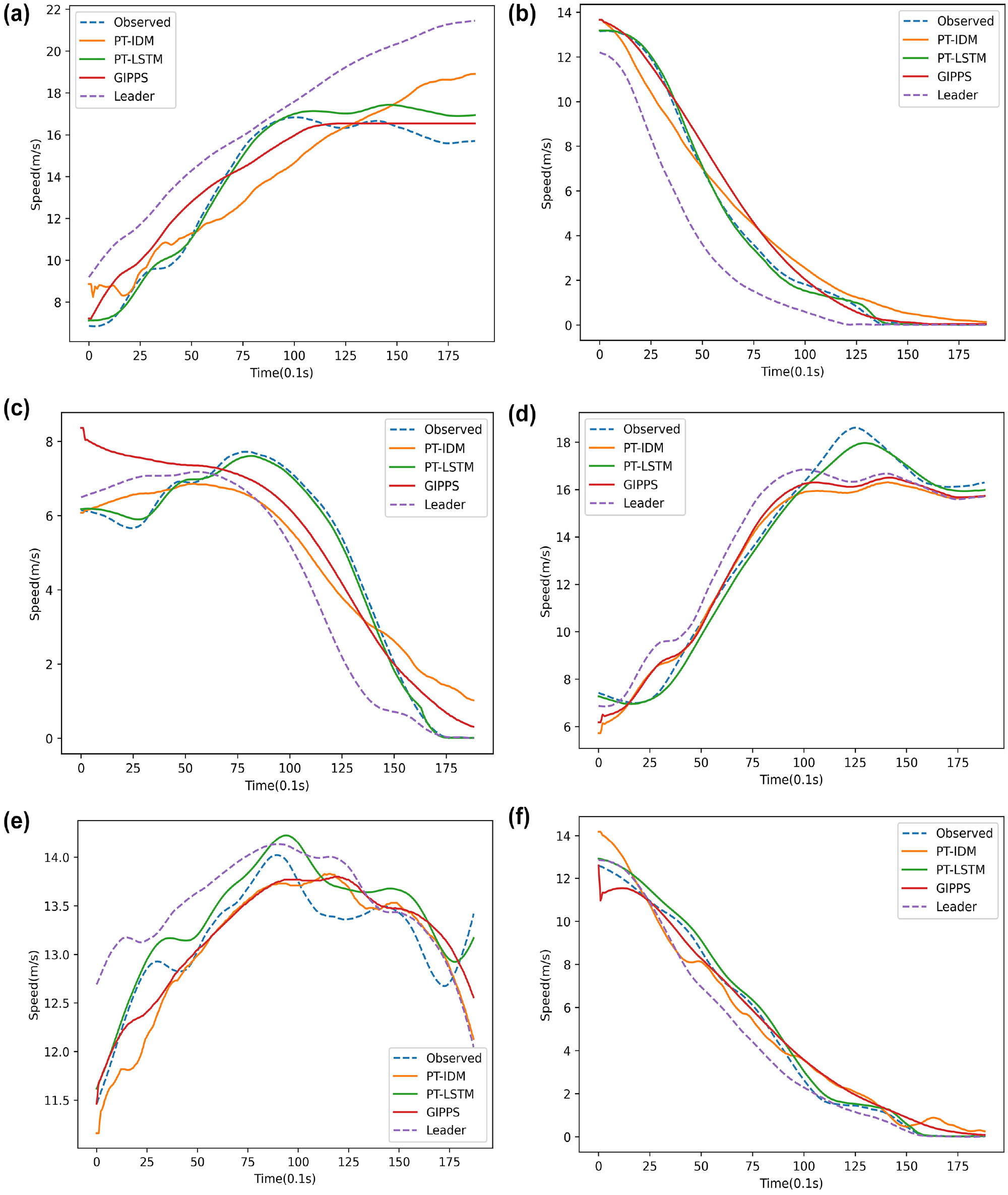
Comparison of observed and predicted following vehicle speed between PT-LSTM model and PT-IDM: (a) AV–HDV (Vehicle Pair 1), (b) AV–HDV (Vehicle Pair 2), (c) HDV–AV (Vehicle Pair 3), (d) HDV–AV (Vehicle Pair 4), (e) HDV–HDV (Vehicle Pair 5), and (f) HDV–HDV (Vehicle Pair 6).
Conclusions and Recommendations
This study extended a data-driven car-following model for HDVs and AVs in AV–HDV mixed-traffic environments. This extended car-following model predicted the following vehicle’s velocity considering how drivers’ (or AVs’) cooperation with the lead vehicle and memory affected their car-following behavior for three groups of lead and following vehicle pair: an AV following an HDV (AV–HDV), an HDV following an AV (HDV–AV), and an HDV following an HDV (HDV–HDV). The cooperation between the lead and following vehicles was modeled using PT and incorporated into the LSTM model as an input. This data-driven car-following model is called the “PT-LSTM model.”
The PT-LSTM model was calibrated using real-world HDV and AV trajectory data extracted from the Waymo Open Dataset. The model parameters were separately calibrated for the three types of vehicle pairs. The calibrated cooperation utility in the PT-LSTM model showed that AV followers were more likely to cooperate with a lead HDV than HDV followers. Moreover, HDV followers were more likely to cooperate with a lead AV than a lead HDV.
The comparison of the PT-LSTM model with the MLP and LSTM models, which do not incorporate PT, revealed that the former achieved a higher prediction accuracy of the following vehicle’s velocity. The PT-LSTM model was additionally evaluated against two mathematical car-following models: the PT-IDM and Gipps’ model. The PT-LSTM model was found to outperform both models in accurately predicting the speed profiles of the following vehicle in AV–HDV, HDV–AV, and HDV–HDV scenarios. This finding underscored that a data-driven car-following model that incorporates cooperation with the lead vehicle and memory, as captured by the PT-LSTM model, can more effectively replicate the car-following behaviors of drivers or AVs in mixed-traffic scenarios.
Furthermore, the SHAP method was utilized to determine the variable importance in the PT-LSTM model at different time steps. The findings revealed that, for all vehicle pair groups, the previous time step’s speed of both the following vehicle and the lead vehicle was important in predicting the following vehicle’s speed in the current time step. However, in the case of the AV–HDV scenario, cooperation utility was found to be more significant than spacing—in contrast to HDV–AV and HDV–HDV scenarios. This observation suggests that AVs were more inclined to cooperate with the lead vehicle, potentially owing to their superior ability to detect the motion of the lead vehicle through sensors compared with HDVs.
However, it should be noted that there are some limitations to the current study. Factors such as road geometries (e.g., slope and curvature) and weather conditions, which can potentially affect car-following behaviors, were not considered. Furthermore, the limited availability of real-world data on AV–AV car-following behaviors may have hindered a comprehensive analysis of AV–AV interactions. Moreover, the transferability of the PT-LSTM model may be limited as it was trained and validated on a specific dataset from Waymo Open Dataset, which may not fully represent all driving conditions or geographic locations. The association of car-following with lane-changing could not be considered because lane-by-lane vehicle trajectory data were not available. Lastly, traffic performance could not be evaluated by applying the PT-LSTM model to a microscopic traffic simulation (e.g., SUMO), similar to the studies by Goncu et al. ( 51 ) and Silgu et al. ( 52 ), as the observed aggregated traffic data were not available. These limitations should be taken into consideration when interpreting the results of this study and in the design of future research.
In future studies, it is recommended that the PT-LSTM model be calibrated for different road geometry, traffic, and weather conditions in AV–HDV mixed traffic, and the behavioral differences between AVs and HDVs and their interactions during car-following be analyzed more extensively. The robustness and transferability of the model could also be evaluated using a wider set of data. It is also recommended that more advanced control strategies of AVs (e.g., CACC) be developed based on the prediction of human driver behaviors in AV–HDV mixed traffic using the PT-LSTM model. In this regard, the PT-LSTM model could be applied to realistic simulation platforms like CARLA to analyze the visual results of AV maneuvers for different control strategies and traffic scenarios.
Footnotes
Author Contributions
The authors confirm contribution to the paper as follows: study conception and design: A. Adewale, C. Lee; data collection: A. Adewale; analysis and interpretation of results: A. Adewale, C. Lee; draft manuscript preparation: A. Adewale, C. Lee. All authors reviewed the results and approved the final version of the manuscript.
Declaration of Conflicting Interests
The authors declared no potential conflicts of interest with respect to the research, authorship, and/or publication of this article.
Funding
The authors disclosed receipt of the following financial support for the research, authorship, and/or publication of this article: This research was supported by Natural Sciences and Engineering Research Council of Canada (Grant no. RGPIN-2019-04430).
Data Accessibility Statement
The data used to support the findings of this study are available in the study by Hu et al. ( 44 ), whereas the code and model are available on request.