Signal Phasing and Timing Prediction Using Connected Vehicle Data

Abstract

Signal phasing and timing can be adaptive and actuated in practice. This makes it challenging to understand what the cycle length and phase duration of the next few cycles will be. Many innovative applications can be designed based on the knowledge of future signal timing states such as dilemma zone warning, efficient route planning, and so forth. This work proposes a long short-term memory model capable of predicting both cycle length and phase duration prediction up to six cycles in the future. GPS information of several vehicles are merged with signal timing information of eight intersections. Several key features such as waiting time, approach speed and acceleration, departing speed and acceleration, are calculated based on the geolocation of individual journeys. The results show that cycle length prediction can reach mean absolute error (MAE) of about 7 s while phase prediction MAE is about 9 s.

Recent advancements in technology have changed the transportation domain significantly since the 2010s. The availability of several new data sources (i.e., sensor technology or vehicle technology) allows for data-driven methodologies that can be incorporated into well-established traffic management systems. In this work, we focus on using deep learning architecture to model signal timing parameters from probe vehicle data. Each approach level volume and occupancy was aggregated at the cycle level from high-resolution detector data. The data were then fed into several machine learning models to compare their performance. Various input-output window sizes were analyzed, to determine the one which is most optimal. Different data preparation methods were also used to calculate the traffic parameters and signal information. Of the five different models tested; long short-term memory (LSTM) gave the best results for mean absolute error (MAE), mean absolute percentage error (MAPE), and root mean square error (RMSE). The proposed model is thoroughly validated on eight different intersections which utilize actuated signal controllers. The model can accurately predict the cycle length and phase duration of the next six cycles which can be instrumental in infrastructure-to-vehicle (I2V) applications. The input data not only consists of traffic features of the target intersection but also considers the features related to the probe vehicle data upstream and downstream of the intersections.

Traditionally, the problem of signal control can be decomposed into a two-stage solution ( 1 ). The first stage is to develop traffic flow models that help to estimate macroscopic traffic parameters at intersections. The next stage is to develop appropriate signal plans based on the estimated traffic flow parameters. The methodology proposed in this paper would aid in reducing the dependency on the optimization algorithms while simultaneously simplifying the traditional two-stage traffic signal control problem into a one-stage solution. A model trained on one intersection can be easily transferred to another intersection, thereby reducing the dependency on signal control optimization. Additionally, most real-time systems, involving delivering signal phasing and timing (SPaT) messages to vehicles, usually have a system delay ( 2 ). This is because the signal states need to travel through several servers to reach the cloud. Data from the cloud is finally sent to the vehicles. In many cases this delay can be so large that information about the next cycle is not readily available. Some of the delay is caused by transmission latency but it is more the result of the way adaptive and actuated signals are programmed. Such signal controllers can extend/reduce cycle length or phase length based on the traffic flow. As such, cycle length and phase length are very dynamic in nature which necessitates some form of prediction algorithm. In the dataset that has been used in this paper, this delay was in between 30 and 60 s. A predictive SPaT model can help to bridge this gap in latency. Moreover, given the time drift of fixed signals and ever-changing traffic condition of adaptive and actuated signals, accurate SPaT information is seldom available ( 3 ). The proposed model can also find applications in connected vehicles where predictive SPaT information can aid in finding optimal routes and in fuel saving.

Literature Review

The literature review is divided into several broad categories to highlight the specific contributions of the current work: review of SPaT prediction, assessment of traffic-related prediction using deep learning, and traffic-related prediction using probe vehicle data. Each of the next paragraphs details the notable work in these three areas.

SPaT Prediction

Many studies have focused on the optimization of signal control ( 4 – 16 ). Some studies have utilized SPaT to find optimal fuel economy ( 17 ) or to guide a vehicle through a signal ( 18 ). Vehicle planning schemes for energy efficiency have also been studied for arterials that predict SPaT based on historical data ( 3 ). SPaT predictions based on GPS data from several buses have been studied by Fayazi et al. ( 19 ) for fixed signal timings. Floating vehicle data from other sources have also been investigated to estimate fixed timing signal parameters by using speed measurements ( 20 – 22 ). A smartphone camera has also been used to detect signal states ( 18 ). Ibrahim et al. ( 23 ) used historical SPaT from a single intersection to calculate future times. Goodall et al. ( 24 ) proposed a microscopic simulation algorithm that utilizes connected vehicle data to obtain future states, which can optimize for delays afterward. That study also mentions that it cannot be implemented in real time because of the computational requirements. A predictive SPaT model is proposed based on vehicles’ arrival time in a connected environment ( 25 ). This method has been only implemented at an isolated intersection, and it was unable to predict beyond the current cycle. As such, it is evident that SPaT predictions at a corridor level using both adaptive and actuated signal control have not yet been studied. SPaT predictions have been explored by Islam et al. ( 26 ) using detector data but not with connected vehicle data.

Assessment of Traffic-Related Prediction Using Deep Learning

Before the advent of deep learning, traffic prediction was conducted by the use of parametric models such as autoregressive models and Kalman filter ( 27 , 28 ) and non-parametric models such as k-nearest neighbor, support vector machine, neural network, and so forth ( 27 , 29 ). In the deep learning era, autoencoders (AE) were first used to show how models can effectively learn existing patterns in data ( 30 , 31 ). Recurrent neural networks (RNN) were also used extensively for traffic parameters like speed, volume, and travel time prediction ( 32 ). LSTM RNNs gathered popularity thereafter because of their memory cells that can decide when to remember past information. Accuracy of prediction also improved by the use of LSTMs even compared with AE and multilayer perceptron (MLP) ( 33 – 35 ). The addition of stacked LSTM layers also further improved the accuracy ( 36 ). Convolutional neural networks (CNN) have also been used to understand traffic flow patterns. Both temporal and spatial features have been used to generate two-dimensional feature sets that can be exploited with CNN ( 37 – 39 ). Several extensions of CNN were also reported to have superior accuracy to traditional CNNs, such as eRCNN ( 40 ) and GraphCNN ( 41 , 42 ). Combinations of several methods have also been used. For example, k-nearest neighbor together with LSTM ( 43 ), AE and LSTM ( 44 ), or CNN and LSTM ( 45 , 46 ). From these studies, it can be concluded that models such as CNN and LSTM are widely used in traffic-related prediction.

Traffic-Related Prediction Using Detector Data

Detector data from various sources such as loop detectors, magnetic and pneumatic tube sensors, radar sensors, infrared sensors, and microwave/radar detectors have also been used in several studies to make traffic-related predictions. Travel time predictions and travel time trends have been studied extensively ( 47 – 50 ). Traffic flow prediction or volume estimation have been studied. Short-term ( 51 – 53 ) and long-term prediction ( 54 – 56 ) has mostly been investigated. Detector data has also been used from camera and loop detectors to predict cycle volumes ( 57 , 58 ). Often advanced detectors can be used to predict speed profiles as well ( 36 , 37 , 39 , 59 , 60 ). Data from smartphones have been used to predict vehicle maneuvers ( 61 ) and activity recognition ( 62 ). In the safety field, several crash risk prediction models have also been proposed and validated using detector data ( 63 – 65 ). Therefore, it can be noted that SPaT predictions have been sparsely studied.

The previous studies discussed have not used real-time detector information for SPaT prediction which provides accurate granular traffic flow for all phases. Additionally, such methods fail to capture the real-time vehicle demand fluctuations in the field and would usually suggest an average solution. The computational requirements of the optimization methods also may not support real-time applications ( 24 ). On the other hand, the LSTM model can be used to make real-time predictions once trained. Additionally, most studies concentrate on one intersection where the reproducibility of the results cannot be understood.

Traffic-Related Prediction Using Probe Vehicle Data

Several studies have been conducted to validate the accuracy and reliability of probe source data ( 66 – 68 ). These found that the quality of data from probe vehicles improved significantly. With high-resolution probe vehicle data, this method has the potential to provide real-time accurate signal timing predictions, based on the variables related to driving behavior, compared to the previous studies. Based on our literature review, there have been limited studies which used probe vehicle data to predict SPaT. However, studies have shown other uses of probe vehicle data. Travel time and speed predictions have been studied extensively ( 69 ). Other studies have also shown the potential for traffic density estimation with probe vehicle data ( 70 ). Each of the studies mentioned above shows the potential that probe vehicle data has to predict many parameters, which are closely related to SPaT prediction.

The proposed work in this paper addresses this research gap and also elaborates on data aggregation at the cycle level from high-resolution probe vehicle data to obtain counts, speeds, and acceleration rates. It also obtains data from traffic signal controllers to calculate cycle length and phase duration. The process of windowing the data and sampling data from the previous day and previous week can also be highlighted as one of the contributions of the paper.

This paper is organized as follows: the next section details the data preparation steps to obtain count, speed, acceleration, and signal parameters. The methodology and model description are presented in the fourth section followed by the results. Finally, discussions about possible applications using this methodology and concluding remarks are made.

Data Preparation

A corridor in Orlando, Florida was selected which operates actuated signal control (SR 434), as shown in Figure 1. It has a total of eight intersections. All eight intersections are equipped with automated traffic signal performance measures (ATSPM) which store high-resolution detector data from each intersection along with the signal timing parameters like cycle length, green time, red time, and so forth. Data from November 11, 2020, to November 17, 2020, were used in the study. Of the eight intersections, two have all protected movements for all phases (Intersections 1295 and 1130). Intersection 1280 does not have protected left turns for the minor road but instead uses dummy phases to balance the ring. Four intersections do not have protected left turns (1285, 1290, 1300, 1305) while Intersection 1275 is a T-intersection. The study area is shown in Figure 1 with the different SignalIDs. ATSPM was used to extract signal and phasing information.

Figure 1.

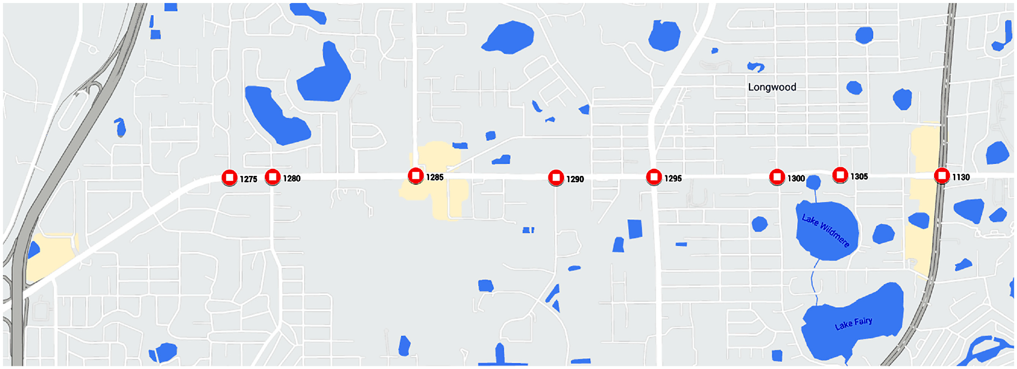
Study area.

Table 1 show the phases that are related to each intersection identity, as well as the direction each phase is tied to, as defined in the ATSPM signal controller database. It also shows the ring diagram that is generally followed for each of the intersections. It should be noted that slightly different ring diagrams are also implemented within the same barrier, depending on the demand at each approach. For example, the through movements may be served only if there is no left-turn demand.

Table 1.

Ring Diagram for the Selected Intersections in the Study Area

Intersection	Ring diagram							Notes	WB-T	EB-T	WB-L	EB-L	SB-T	NB-T	SB-L	NB-L
1275	Ring 1	1	2	8				T-intersection	2	6	-	1	8	-	-	-
	Ring 2		6
1280	Ring 1	1	2	3	4			-	2	6	5	1	8	4	3	7
	Ring 2	5	6	8	7
1285	Ring 1	1	2	3	8	7	4	-	6	2	1	5	4	8	-	-
	Ring 2	5	6
1290	Ring 1	1	2	3	8	7	4	-	2	6	5	1	8	4	-	-
	Ring 2	6	5
1295	Ring 1	1	2	4	3			-	6	2	1	5	4	8	7	3
	Ring 2	6	5	7	8
1300	Ring 1	1	2	4				No protected left for minor road	6	2	1	5	4	8	-	-
	Ring 2	5	6	8
1305	Ring 1	1	2	4				No protected left for minor road	6	2	1	5	4	8	-	-
	Ring 2	5	6	8
1130	Ring 1	1	2	3	4			-	6	2	1	5	4	8	7	3
	Ring 2	6	5	7	8

Note: EB = eastbound; NB = northbound; SB = southbound; WB = westbound; L = left; T = through; “-” = not applicable/no data.

The connected vehicle (CV) data used in this paper were provided by the CV data service, Wejo. The data set contains vehicle-specific data from several manufacturers. It mainly has non-commercial fleet data which better represents the vehicles on the roadways. Instantaneous data is sent from the vehicle to the cloud in near real time. The dataset consists of GPS location, heading, speed, postal code, journeyId and dataPointId. The sampling rate of the dataset was limited to 3 s. One week of data was used in this study, the week of November 11–17, 2019. The entire dataset had a total of 100 million GPS points. The CV data was processed according to the pipeline shown in Figure 2. The CV data points were spatially filtered to obtain the trajectories within 330 ft of the selected eight intersections. The arrival time was estimated when a vehicle entered the 330 ft buffer, and the departure time was when the vehicle left the buffer. Based on the arrival and departure, approaching acceleration and speed as well as departing acceleration and speed was computed for each journey. Whether that trajectory waited at the intersection was also estimated from the speed profile. The approaching direction and departing directions were also computed since they will give an indication of the particular phase the vehicle used.

Figure 2.

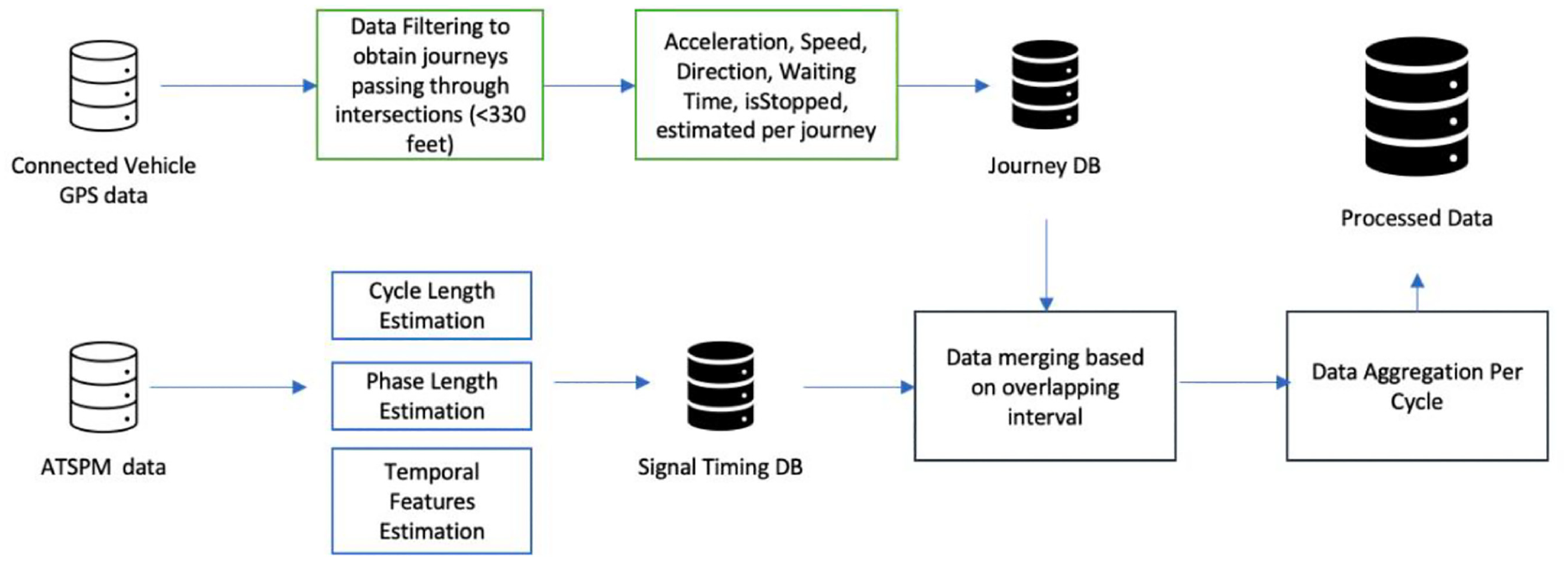
Data processing pipeline.

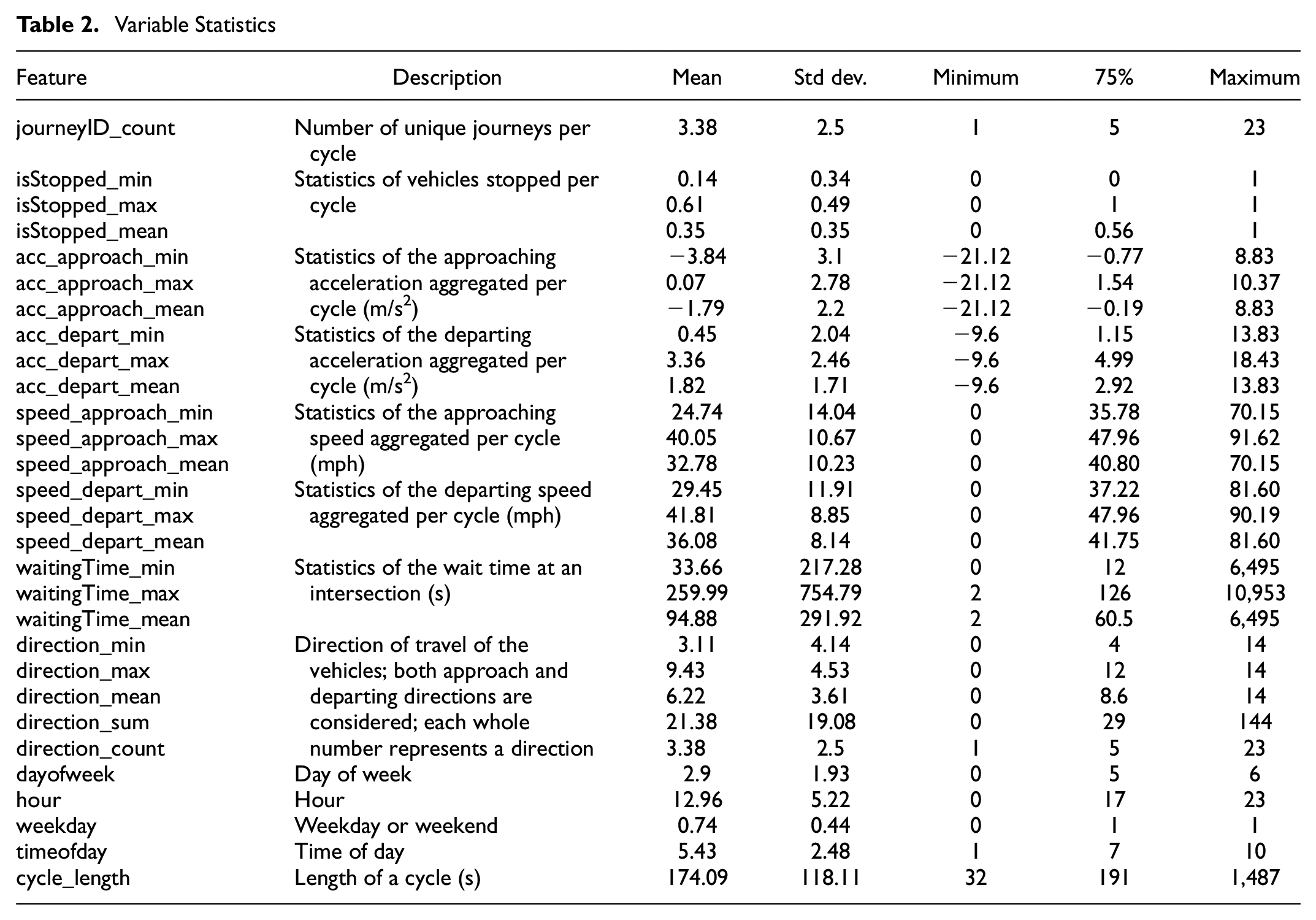
Meanwhile, the ATSPM data were processed to extract cycle lengths and phase lengths. Temporal features such as hour, day of week, weekend/weekday, and so forth were also measured. The cycle start time and end time were also noted. The two datasets were merged based on overlapping timestamps. For instance, if the arrival time of a Wejo vehicle is 10:10:12 within the buffer area, and the cycle start time and end time is 10:10:11 and 10:10:14, then this particular vehicle would be considered to use this cycle. The vehicle dynamic features such as speed, acceleration, direction, and so forth were also used as features for this cycle. Finally, the individual journeys were aggregated per cycle to provide information on the number of vehicles that used the cycle, the direction of travel as well as the vehicle dynamics such as aggregated acceleration and speed. This resulted in 18,790 journeys that used the intersection with the study period. The different features estimated are shown in Table 2. Cycle lengths greater than 1,500 s were discarded since this can usually happen at unsaturated condition at nighttime or from detector failure; 95% of the cycle lengths were within 350 s. The journeyID_count is the number of vehicles that have used a cycle. The maximum is shown in the table as 22, which is lower than the expected maximum volume. The penetration rate of CVs was around 3% during the study period.

Table 2.

Variable Statistics

Feature	Description	Mean	Std dev.	Minimum	75%	Maximum
journeyID_count	Number of unique journeys per cycle	3.38	2.5	1	5	23
isStopped_min	Statistics of vehicles stopped per cycle	0.14	0.34	0	0	1
isStopped_max		0.61	0.49	0	1	1
isStopped_mean		0.35	0.35	0	0.56	1
acc_approach_min	Statistics of the approaching acceleration aggregated per cycle (m/s2)	−3.84	3.1	−21.12	−0.77	8.83
acc_approach_max		0.07	2.78	−21.12	1.54	10.37
acc_approach_mean		−1.79	2.2	−21.12	−0.19	8.83
acc_depart_min	Statistics of the departing acceleration aggregated per cycle (m/s2)	0.45	2.04	−9.6	1.15	13.83
acc_depart_max		3.36	2.46	−9.6	4.99	18.43
acc_depart_mean		1.82	1.71	−9.6	2.92	13.83
speed_approach_min	Statistics of the approaching speed aggregated per cycle (mph)	24.74	14.04	0	35.78	70.15
speed_approach_max		40.05	10.67	0	47.96	91.62
speed_approach_mean		32.78	10.23	0	40.80	70.15
speed_depart_min	Statistics of the departing speed aggregated per cycle (mph)	29.45	11.91	0	37.22	81.60
speed_depart_max		41.81	8.85	0	47.96	90.19
speed_depart_mean		36.08	8.14	0	41.75	81.60
waitingTime_min	Statistics of the wait time at an intersection (s)	33.66	217.28	0	12	6,495
waitingTime_max		259.99	754.79	2	126	10,953
waitingTime_mean		94.88	291.92	2	60.5	6,495
direction_min	Direction of travel of the vehicles; both approach and departing directions are considered; each whole number represents a direction	3.11	4.14	0	4	14
direction_max		9.43	4.53	0	12	14
direction_mean		6.22	3.61	0	8.6	14
direction_sum		21.38	19.08	0	29	144
direction_count		3.38	2.5	1	5	23
dayofweek	Day of week	2.9	1.93	0	5	6
hour	Hour	12.96	5.22	0	17	23
weekday	Weekday or weekend	0.74	0.44	0	1	1
timeofday	Time of day	5.43	2.48	1	7	10
cycle_length	Length of a cycle (s)	174.09	118.11	32	191	1,487

Model

Several models were evaluated alongside LSTM: random forest, support vector machine, gradient boosting and extreme gradient boosting. Brief descriptions of the models are provided in this section followed by comparative results.

Random Forest

Random forest (RF) is a tree-based classifier that employs two distinct machine learning techniques: random feature selection and bagging ( 71 ). Random feature collection creates decision trees immediately, whereas bagging creates each tree separately. A decision tree model starts at the root node and splits the data on the features that result in the largest information gain. This partition process is repeated iteratively until the child node is optimized to have values that belong to the same class ( 72 ). Rather than employing all of the features in the decision trees, RF selects the features of the subsets at random. For forecasting the output of a new dataset, RF uses the mean value of the outputs from random independent bootstrap training data.

Support Vector Machine

The support vector machine (SVM) method is a supervised learning algorithm that is widely used. Given a data set D in the form of ${\{{\mathrm{x}}_{\mathrm{i}},{\mathrm{y}}_{\mathrm{i}}\}}_{\mathrm{i}=1}^{\mathrm{N}}$ , where ${\mathrm{x}}_{\mathrm{i}}ϵ{\mathrm{R}}_{\mathrm{d}}$ are the samples, and the ${\mathrm{y}}_{\mathrm{i}}$ is the label, SVM maps the feature vector ${\mathrm{x}}_{\mathrm{i}}$ to an N-dimensional space, with N as the number of features of the samples. For a multiclass classification problem, SVM breaks down the multiclassification problem into multiple binary classification problems and finds the hyperplane (decision boundary) to distinctly separate the multiple classes of samples. The distance between the two classes is regarded as the margin distance. SVM uses a loss function to maximize the margin distance, which is to solve Equation 2:

$$\mathrm{J}=min\frac{1}{2}{\mathrm{w}}^{\mathrm{T}}\mathrm{w}+\mathrm{C}\sum _{\mathrm{i}=1}^{\mathrm{N}}{\mathrm{\epsilon }}_{\mathrm{i}}$$

(1)

subject to:

$${\mathrm{y}}_{\mathrm{i}}({\mathrm{w}}^{\mathrm{T}}{\mathrm{K}}_{\mathrm{i}}\left({\mathrm{x}}_{\mathrm{i}}\right)+\mathrm{b})\ge 1-{\mathrm{\epsilon }}_{\mathrm{i}}$$

where w is weight vector, C is cost coefficient, and ${\mathrm{\epsilon }}_{\mathrm{i}}$ is a slack variable for the non-separable data, and K_i is the kernel function to transform data to the feature space. There are different kernel functions to use, such as linear functions, radial basis functions, and so forth.

Gradient Boosting

Gradient boosting model (GBM) is a machine learning method that utilizes many decision trees (weak learners) to generate results. For GBM, at each iteration a new tree is added. The subsequent trees will give extra weights to the samples that are incorrectly classified by the prior tree. Residuals are added to generate the final classification result based on all the trees ( 73 ).

Extreme Gradient Boosting

XGBoost (eXtreme Gradient Boosting) is an extension of the popular tree gradient boosting algorithms ( 74 ). Boosting is the mechanism to add models recursively until optimal performance metrics are achieved. In gradient boosting, new models are added that predict the residuals of the prior which are added together for the final prediction. XGBoost has been proven to be an efficient and scalable version of gradient boosting trees that is also capable of utilizing maximum memory and hardware resources for data intensive models. It is also able to integrate sparsity aware data handling capabilities as well as a weighted quantile sketch for approximate learning as shown by Chen and Guestrin ( 75 ). The authors were also able to generate a scalable package by gaining insights on cache access patterns, data compression, and sharding that aided in training billions of samples with the more meager of resources.

Mathematically XGBoost is summarized with Equations 2 to 4.

$$\mathrm{f}={\mathrm{\omega }}_{\mathrm{q}\left(\mathrm{x}\left(\mathrm{t}\right)\right)}$$

(2)

$${\mathrm{L}}^{\left(\mathrm{t}\right)}=\sum _{\mathrm{i}=1}^{\mathrm{n}}\mathrm{l}({\mathrm{y}}_{\mathrm{i}},{\hat{\mathrm{y}}}_{\mathrm{i}}^{\mathrm{t}-1}+{\mathrm{f}}_{\mathrm{t}}\left({\mathrm{x}}_{\mathrm{i}}\right))+\mathrm{\Omega }\left({\mathrm{f}}_{\mathrm{t}}\right)$$

(3)

$$\mathrm{\Omega }\left({\mathrm{f}}_{\mathrm{t}}\right)=\mathrm{\Upsilon }\mathrm{T}+0.5*\mathrm{\lambda }\sum _{\mathrm{i}=1}^{\mathrm{T}}{\mathrm{\omega }}_{\mathrm{i}}^2$$

(4)

where $\mathrm{x}\left(\mathrm{t}\right)$ is the input data, ${\mathrm{y}}_{\mathrm{i}}$ is the target variable while ${\hat{\mathrm{y}}}_{\mathrm{i}}$ is the predicted value for the i-th sample, $\mathrm{q}$ is the function that maps a sample into a tree structure, $\mathrm{\omega }$ is the leaf weight, $\mathrm{T}$ is the number of leaf nodes, $\mathrm{L}$ is the loss function, $\mathrm{\Upsilon }$ and $\mathrm{\lambda }$ are the regularization parameters.

LSTM

LSTM networks ( 76 ) belong to the RNN family and are adept at overcoming the shortcoming of conventional RNN: the vanishing gradient problem. This limitation means that RNNs can remember only recent information. LSTM can make use of both short-term and long-term information to make a prediction. This is especially important in the prediction of signal timing because generally optimizations are done by considering both the short-term turbulent traffic flow and the long-term mean traffic parameters. LSTMs have an input layer, a hidden layer, and an output layer. While the input and output layers are traditional neurons, the hidden layers are specialized memory cells that can store information.

For the input of sequence $x_t$ and $i,o,f,c$ as the input gate, output gate, forget gate, and cell input of LSTM, the hidden layer function ( 77 ) can be formulated as in Equations 5 to 9.

$$i_t=\sigma (W_{\mathrm{xi}}{x}_t+W_{\mathrm{hi}}{h}_{t-1}+W_{\mathrm{ci}}{c}_{t-1}+b_i)$$

(5)

$$f_t=\sigma (W_{\mathrm{xf}}{x}_t+W_{\mathrm{hf}}{h}_{t-1}+W_{\mathrm{cf}}{c}_{t-1}+b_f)$$

(6)

$$i_t=f_t{c}_{t-1}+i_t\tanh (W_{\mathrm{xc}}{x}_t+W_{\mathrm{hc}}{h}_{t-1}+b_c)$$

(7)

$$o_t=\sigma (W_{\mathrm{xo}}{x}_t+W_{\mathrm{ho}}{h}_{t-1}+W_{\mathrm{co}}{c}_{t-1}+b_o)$$

(8)

$$h_t=o_t\tanh \left(c_t\right)$$

(9)

where $\sigma$ is the logistic sigmoid function and $h$ is the hidden vector. The weight matrices are represented with $W$ . $W_{\mathrm{xo}}$ is the weight matrix of the input-output gate matrix, $W_{\mathrm{xf}}$ is that of input-forget gate, and so forth. A typical structure of LSTM cell is shown in Figure 3 and the proposed network architecture is shown in Figure 4. The model has four stacked LSTM layers followed by one dense layer. Several hyperparameters, such as number of LSTM and dense cells, learning rate, batch size, and so forth, were also selected and the best one was chosen based on the evaluation metrics.

Figure 3.

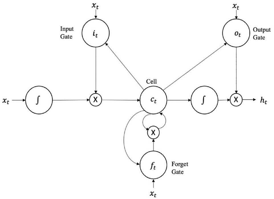
Long short-term memory (LSTM) cell structure.

Figure 4.

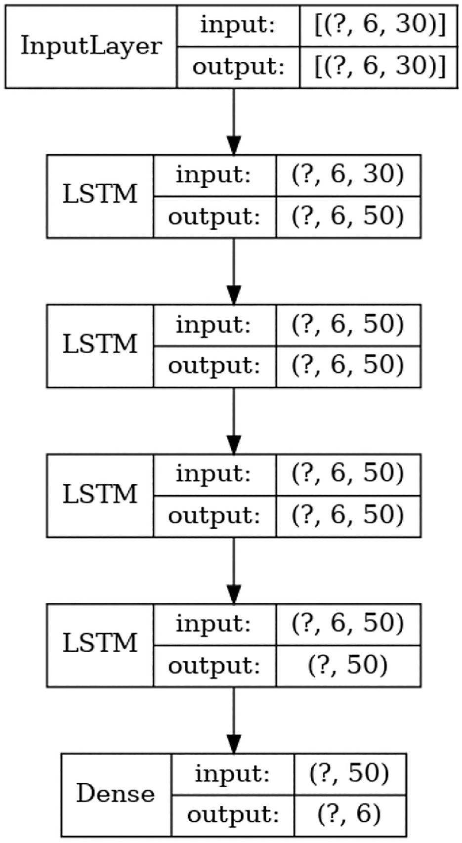
Long short-term memory (LSTM) architecture.

Results

Performance metrics were evaluated for individual intersection models as well as combined intersection models. MAE, MAPE, and RMSE were taken as the metrics and calculated with Equations 10 to 12, where ${\hat{y}}_i$ is the predicted values and $y_i$ is the actual values.

$$\mathrm{MAE}=\frac{\sum _{i=1}^n|y_i-{\hat{y}}_i|}{n}$$

(10)

$$\mathrm{MAPE}=\frac{1}{n}\sum _{i=1}^n\frac{|y_i-{\hat{y}}_i|}{x_i}$$

(11)

$$\mathrm{RMSE}=\sqrt{\frac{\sum _{i=1}^n{(y_i-{\hat{y}}_i)}^2}{n}}$$

(12)

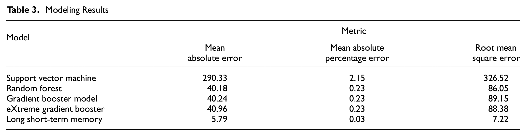
The performance of all the models for the cycle length prediction is shown in Table 3. It can be noted that LSTM is the best performing model in MAE, MAPE and RMSE. The tree-based models such as RF, GBM, and XGBT models returned similar results, with the MAE about 40 s, MAPE at 23%, and RMSE around 85 s. Since the average cycle length is 174 s in the processed data set, these models will have average predictions between 134 and 214 s. The results from LSTM are much better, with a MAE of 5.79 s. It is important to note here that all these model results are compared based on the current cycle length prediction. The impact of window lengths is explored in the next part of the results.

Table 3.

Modeling Results

Model	Metric
	Mean absolute error	Mean absolute percentage error	Root mean square error
Support vector machine	290.33	2.15	326.52
Random forest	40.18	0.23	86.05
Gradient booster model	40.24	0.23	89.15
eXtreme gradient booster	40.96	0.23	88.38
Long short-term memory	5.79	0.03	7.22

The impact of input and output window sizes are also explored with the best performing model, LSTM. Two input window sizes are taken, 5 and 6, while the output window size is varied from 1 to 6. For instance, in Table 4, “5,4” means that the model takes the last five cycles’ information and predicts the cycle length and phase length of the next four cycles. In Table 4, both cycle length prediction and phase duration prediction results are shown. For the phase prediction, the model predicts all the phases as individual output. If the prediction window is 4 s, there will be eight phase predictions pre-cycle for a total of 32 phases for the entire output. The results have acceptable performance with the minimum MAE for “6,2” in cycle length prediction (7.16 s) and “6,6” for phase length prediction (8.71 s). It should also be noted that for the phase length prediction, the MAPE is always over 40% even though the MAE is always below 10 s. The reasoning is that sometimes a particular phase will ideally remain closed when there is no demand and phase length is then 0 s. If the model outputs a prediction of 0.4 s, that will lead to a 40% error. The true values and predicted values were plotted on a graph to identity this abnormal error even though the MAE was good. A way to mitigate this error could be to round unreasonably small phase lengths to zero.

Table 4.

Cycle Length and Phase Length Prediction Performance

	Window	5,1	5,2	5,3	5,4	5,5	6,1	6.2	6,3	6,4	6,5	6,6
Cycle length	MAE	12.34	11.39	17.82	18.73	6.51	9.22	7.16	21.6	21.68	9.25	19.7
	MAPE	0.04	0.39	0.05	0.06	0.06	0.01	0.05	0.07	0.13	0.04	0.10
	RMSE	14.43	14.56	19.88	20.61	8.17	11.37	9.12	23.88	25.92	11.34	23.02
Phase length	MAE	9.32	9.08	9.02	8.83	8.95	9.14	8.77	9.00	8.79	8.81	8.71
	MAPE	0.78	0.49	0.40	1.43	0.41	1.19	0.49	0.49	0.57	0.57	0.41
	RMSE	19.14	19.43	18.80	18.19	18.87	19.66	17.95	18.23	18.73	18.65	17.76

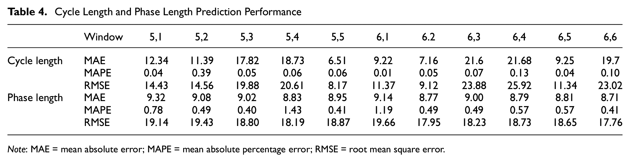
Note: MAE = mean absolute error; MAPE = mean absolute percentage error; RMSE = root mean square error.

To understand the importance of the variables, we computed the effect of the prediction when there is a perturbation in the input features. The inputs are perturbed with a random normal distribution centered at zero with a standard deviation of 0.2. The RMSE of the predictions and the ground truth are then compared. The larger the RMSE the more the perturbation and thus the more it is important for the model. The results are shown in Figure 5. It can be noted that the intersection identity of each signal is the most significant factor. Since each intersection experiences different traffic flow and each also has different numbers of lanes and other geometric features, it is likely that the model interprets this identity to be an important feature. Therefore, transferability of the model would be dependent on these factors. The other significant features include various speed and acceleration metrics as well as the number of vehicles (journeyID_count), as well as waiting time of each vehicle.

Figure 5.

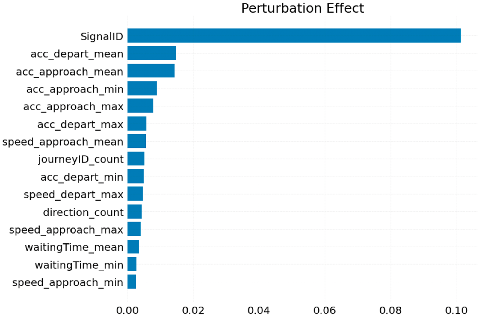
Feature importance using perturbation.

Conclusion

This work proposed the use of CV data to predict SPaT information. SPaT information from several intersections was collected for a week in November 2019 alongside several GPS coordinates of individual vehicles. A buffer of 330 ft around each intersection was selected to identify the approaching and departing vehicles within an intersection and several features were calculated. The individual journeys were then aggregated per cycle along with cycle length and phase duration information from ATSPM data. The prediction model based on LSTM was then used to predict up to six cycles in the future. Various input and output window lengths were experimented with and MAE, MAPE, and RMSE were taken as metrics for evaluation. The LSTM model outperformed the other models such as SVM, RF, GBM, and XGBT. The MAE, MAPE, and RMSE for the LSTM model were 5.79 s, 0.03%, and 7.22 s respectively for cycle length prediction and 8.83 s, 1.43%, and 18.19 s for phase length prediction.

Overall, SPaT prediction can help to deploy real-time traffic safety and mobility features. Often in complicated urban settings, even high-speed internet facilities cannot deliver SPaT messages in real time. A study by Goodall et al. ( 24 ) proposes an algorithm that can optimize delay by using CV data but also notes that it cannot be applied in real time because of the computational requirements. The future forecast of the SPaT timings can be relied on in such cases. It can aid in overcoming the system delay in processing and broadcasting SPaT messages. Moreover, traffic flow prediction or speed prediction can also be improved, for the case of arterials, if future signal states are known. In such cases, improving the prediction by even a few seconds can prove to be useful. Furthermore, a new intersection with similar traffic flow parameters may benefit from a trained model of a totally different intersection. While the proposed methodology cannot rule out signal optimization altogether, it can easily aid relevant authorities to replicate a well-performing signal timing to other intersections easily.

There are many potential applications of predicting the SPaT timing of the upcoming cycles. It can make route planning and trajectory estimation ( 78 ) more efficient in a connected environment since future states of the signals can be predicted. This would aid in relevant studies where vehicle velocity is optimized to traverse intersections at green times, thereby reducing the carbon footprint ( 17 ), or to find optimal velocity ( 18 ). The predicted signal timings can also be used to aid vehicles in the dilemma zone if the predictions can be transferred to the vehicles using onboard units. Most prominently, the signal retiming effort can be reduced to a great extent. Recent studies related to safety that try to predict pedestrian and vehicle conflicts using signal timing information ( 79 , 80 ) can also benefit from having extended SPaT information up to six cycles in the future.