Sage Journals: Discover world-class research

Abstract

Use of the multinomial logit (MNL) functional form is widespread in transportation and land use demand modeling. As the state-of-the-art evolves away from aggregate forecasting and toward activity-based models and microsimulation, MNL models are being asked to accommodate increasingly large choice sets. Different strategies exist to address the challenge of estimating models with very large choice sets, but perhaps none is as commonly employed as sampling of alternatives. The effect of sampling of alternatives on parameter estimation has received considerable attention in the scientific literature. Yet comparatively little quantitative research exists that examines the issues that arise when the same sampling strategies are applied in the context of forecasting. In this study we conducted an analysis of the effect of sampling of alternatives in discrete choice models for disaggregate location choice forecasting. First, a novel measure of forecast error was defined and then used to quantify the extent of the problem as a function of sample rate, model error, and size of the universe of alternatives. Finally, we explored the potential for strategic sampling techniques to reduce the error observed under simple random sampling. In general, we found that the proportion of aggregate demand that was misallocated owing to sampling of alternatives was actually reduced as the size of the universe of alternatives increased. Additionally, simple random sampling was shown to outperform importance sampling in most scenarios. These findings suggest that error resulting from random sampling of alternatives is less of a problem for logit-based microsimulation models than previously assumed.

Keywords

data and data science statistical methods modeling planning and analysis travel demand modeling

Use of the multinomial logit (MNL) discrete choice model is widespread in transportation and land use demand modeling, both in the research literature and in applied settings. As the state-of-the-art continues to evolve away from aggregate forecasting and toward activity-based models and microsimulation, MNL models are being asked to accommodate increasingly large choice sets ( 1 , 2 ). Different strategies exist to address the challenge of estimating models with very large choice sets, but perhaps none is as commonly employed as sampling of alternatives. The effect of sampling of alternatives on model estimation has received considerable attention in the scientific literature ( 3 – 5 ). Yet comparatively little quantitative research exists that examines the issues that arise when the same sampling strategies are applied in the forecasting or simulation phase of the modeling process.

Despite a lack of empirical evidence, it is often assumed that sampling strategies that improve parameter estimates must also improve the accuracy of demand forecasts as well. The current study tested the validity of this assumption by defining a new empirical measure of prediction error and using it to evaluate outcomes under different modeling scenarios and sampling strategies. The mathematical definition of this prediction error metric is itself a valuable contribution to the scientific literature on a topic that is rarely studied, in part because of how challenging it is to measure model error without the benefit of observed choices, as is almost always the case for forecasting. Just as important, however, are the experimental results, which can help practitioners navigate the tradeoffs between sample rate and aggregation of alternatives under fixed computational resources.

Background

The use of sampling of alternatives in logit models with large choices dates back to McFadden, who showed that consistent MNL estimates for a parameter vector, $β^{*}$ , can be obtained using a sample of nonchosen alternatives by adding an alternative-specific correction term to the standard logit choice model ( 6 ),

p_{n} (i | D_{n}) = \frac{e^{μ β^{⊤} X_{in} + \ln π_{n} (D_{n} | i)}}{\sum_{j \in D_{n}} e^{μ β^{⊤} X_{jn} + \ln π_{n} (D_{n} | j)}}, \forall D_{n} \subset C

(1)

The term $\ln π_{n} (D_{n} | i)$ is called the correction factor and represents the likelihood of constructing choice set $D_{n}$ conditional on chooser $n$ selecting alternative $i$ . Under simple random sampling (SRS) this term is equal for all alternatives, $j$ ,

π_{n} (D_{n} | i) = π_{n} (D_{n} | j) \forall i, j \in D_{n}

(2)

This “uniform conditioning property” causes the correction factors in the numerator and denominator of Equation 1 to cancel out, allowing the use of the simplified logit form instead,

p_{n} (i | D_{n}) = \frac{e^{μ β^{⊤} X_{in}}}{\sum_{j \in D_{n}} e^{μ β^{⊤} X_{jn}}}

(3)

The simplicity of this model, and that $β^{*}$ has a closed form solution under maximum likelihood estimation, has led to its proliferation among practitioners of travel and land use demand modeling.

Consistency of parameter estimates does not imply that they are also efficient, which, as it relates to sampling of alternatives, depends on the size and composition of the sample. The relationship between sampling of alternatives and model error has been quantified extensively (3 –5, 7 ). Researchers have also found success developing and applying alternative sampling strategies that are able to improve parameter efficiency by oversampling alternatives deemed most relevant to a particular choice context ( 3 , 8 –11).

Although the effect of sampling of alternatives in discrete choice models seems well understood, the problem space is much murkier for practitioners who, having estimated a model, must actually use it to perform scenario analyses or generate regional forecasts. The key distinguishing factor is that there are no “observed” choices in the context of such predictive modeling. This fact has two important consequences, which served as the motivation for this study. The first is that sampling of alternatives may produce choice sets composed entirely of unattractive or “uninformative” alternatives with small probabilities ( 12 ). Importantly, the likelihood of generating such a sample increases with the size of the universe of alternatives ( 3 , 13 ), which suggests that the problem may be most severe for microsimulation models in which choice sets commonly number into the millions of alternatives and random sampling of alternatives is heavily relied on ( 1 , 14 –16).

The second consequence is that there is no straightforward way to assess performance in the forecasting phase of the modeling lifecycle. Intuitively, there can be no “ground truth” for a model designed to predict outcomes under scenarios that have not yet come to pass. This is especially true when the choices being modeled are those of a synthetic population, as is often the case in microsimulation and activity-based models. As a result, the study of forecast error in discrete choice models has focused almost entirely on reducing parameter error under the assumption that what is good for the estimation goose must also be good for the simulation gander. Two exceptions are worth mentioning. The first is Jones et al., which studies the effect of aggregation of alternatives on forecasting error for location choice models ( 17 ). In that study, the authors explicitly describe why variation in parameter estimates cannot reliably measure predictive performance in the forecasting phase. The principal reason cited is that error in the individual parameter estimates can balance itself out across parameters, and across alternatives, too. Furthermore, if in practice a modeler is primarily concerned with the spatial distribution of demand, then it is possible for this error to balance itself out across choosers as well. In this sense, the net effect could therefore be significantly less than the estimation error would indicate.

The second study is by Guevara and Ben-Akiva, which investigates methods for reducing forecasting error owing to endogeneity bias ( 18 ). Importantly, the authors point out that “predictions at a disaggregated level are almost always meaningless,” and advocate instead for assessing microsimulation performance at an aggregate level. Although aggregating the results of a disaggregate model may seem self-defeating, it is not. Since the inception of microsimulation for policy analysis ( 19 ), practitioners have stressed that its value over aggregate modeling lies in its ability to more accurately predict the distribution of demand across a population of individuals, not chooser-level outcomes ( 20 ). This is in large part a result of the highly stochastic nature of microsimulation, which, far from being a shortcoming of the approach, is actually one of the features that allows it to incorporate the effects of population heterogeneity, emergent behaviors, and other low probability outcomes. In practice, this stochastic variation (also called Monte Carlo error [ 21 ]) is typically handled by running the model(s) multiple times with different seeds supplied to the random number generators, and taking the average of the results ( 2 ). It follows, therefore, that any metric used to quantify forecasting error must focus on aggregate demand for alternatives across a population, and must utilize the entire distribution of choice probabilities for each chooser rather than just that of the highest utility alternative or the alternative selected via Monte Carlo simulation.

Key Questions and Contributions of this Study

This study first defines and then applies a novel measure of prediction error to investigate the following three research questions: 1) How does error from sampling of alternatives change as the size of the universe of alternatives increases by orders of magnitude? 2) Does error from random sampling of alternatives balance itself out across choosers in relation to aggregate demand? 3) Can forecast error be reduced by replacing SRS with a strategically weighted sampling approach?

In regard to the first question, we hypothesized that error would be largest at the most disaggregate scales, where choice sets can number in the millions of alternatives. This hypothesis was informed by previous work that has shown that it is easier to sample “non-competitive alternatives” when choice sets are largest ( 3 ). In the estimation phase, this leads to greater parameter error. In forecasting, however, we would expect inefficient choice sets to result in overassignment of choosers to low-utility alternatives, and therefore an overdispersion or diffusion of aggregate probability across alternatives relative to the true distribution one would obtain from a 100% sample. In a model of residential location choice, for example, this might manifest as underpredicted population densities for the most attractive locations. Figure 1 illustrates an idealized version of this phenomenon, which we term “dispersion error.”

Figure 1.

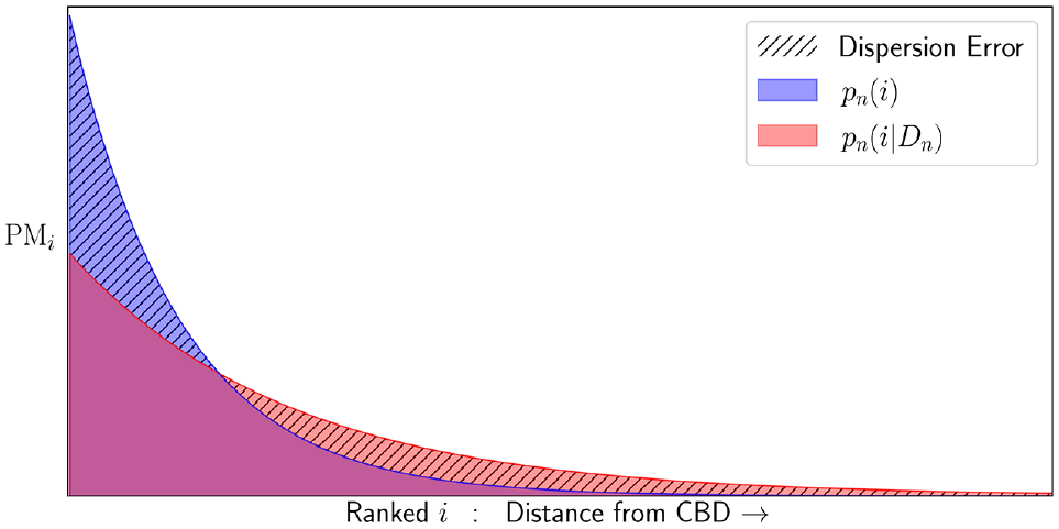
Graphical representation of dispersion error in a location choice model for an idealized monocentric city with random sampling of alternatives for a single chooser, n. The area of both the blue and red distributions is equal to one since each is a probability density function. The theoretical upper limit of dispersion error is therefore two, which would occur if the distributions had zero overlap.

It is more difficult to speculate about the second question since it has no analog in the literature on model estimation. Research has shown that even with random sampling of alternatives, discrete choice microsimulations can achieve greater predictive accuracy than traditional aggregate models ( 22 ). But no study until now has managed to isolate the effect of sampling of alternatives on forecasting error in a way that can guide practitioners who must navigate the tradeoff between computation time and sample size. If in fact the sample error that is associated with microsimulation is balanced out (i.e., mean zero) when aggregating demand across choosers, then the marginal benefit of using larger sample sizes should decrease past a certain point. By using an aggregate metric like dispersion error to compare the performance of a single disaggregate model at multiple sample rates, this study was able to test the hypothesis and determine whether such a threshold exists.

The expected outcome of the third research question follows from the first, in that importance sampling would be expected to increase the likelihood of constructing choice sets with high-utility alternatives, thereby reducing dispersion error. We also hypothesized that the benefit of importance sampling would be greatest for the largest choice set scenarios where we expected the overall error owing to sampling of alternative to be most severe.

The rest of the paper is structured as follows. We first provide a mathematical definition of dispersion error for measuring error resulting from sampling of alternatives in MNL forecasting. We next describe the experimental design, including the generation of synthetic data from MNL models of our own design. The use of synthetic data meant no model estimation was required, and the effect of sampling of alternatives on parameter efficiency could be ignored. Instead, dispersion error was measured by repeatedly simulating choice probabilities using different sample sizes between 2 and $J - 1$ , where $J$ is the number of alternatives in the universal choice set, and comparing the distribution of aggregate choice probabilities to that obtained from a 100% sample. We also defined the boundary conditions of the experiment through the use of three experimental controls: 1) the size of $J$ ; 2) the variance of the model error; and 3) the sample rate. This procedure was then repeated using an important sampling strategy to explore how alternative techniques to random sampling of alternatives can be used to reduce dispersion error. Lastly, we contextualized these findings by repeating this procedure using a location choice model estimated from real data.

Methodology

Measuring Dispersion Error

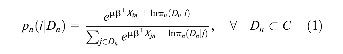
Let us first define the probability of chooser n selecting alternative $i$ from the universal choice set, $N$ , with $J$ elements using the standard MNL model formulation

p_{n} (i) = \frac{e^{μ V_{in}}}{\sum_{j \in C} e^{μ V_{jn}}} = \frac{e^{μ β^{⊤} X_{in}}}{\sum_{j \in C} e^{μ β^{⊤} X_{jn}}}, i = 1, \dots, J

(4)

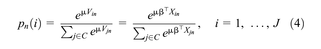
where $V_{in}$ represents the structural component of the utility function

U_{in} = V_{in} + ϵ_{in}, ϵ ~ Gumbel (0, μ)

(5)

and is itself defined as a linear combination of parameter vector $X_{in}$ with a vector of fixed coefficients, $β$

V_{in} = β^{⊤} X_{in}

(6)

We define the aggregate demand for alternative i across the population of choosers, $N$ , as the probability massing,

P M_{i} = \sum_{n} p_{n} (i), 0 \leq P M_{i} \leq N

(7)

which incorporates the total choice probability for each alternative regardless of whether a chooser would be predicted to select it under Monte Carlo simulation.

The best outcome when simulating choices under sampling of alternatives is to replicate the empirical distribution of aggregate probability obtained without sampling. Therefore, we defined the probability massing error (PME) resulting from sampling of alternatives for alternative as the difference between the best-case-scenario probability massing (no sampling) and that obtained from the conditional logit probabilities $p_{n} (i | D_{n})$ :

\begin{matrix} PM Erro r_{i} = \sum_{n} p_{n} (i | D_{n}) - \sum_{n} p_{n} (i) \\ where p_{n} (i | D_{n}) = {\begin{matrix} \frac{e^{μ V_{in}}}{\sum_{j \in D_{n}} e^{μ V_{jn}}} if i \in D_{n}, \\ 0 otherwise \end{matrix} D_{n} \subset C \end{matrix}

(8)

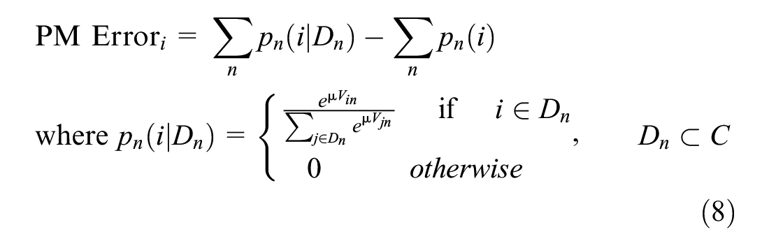
An additional benefit of aggregation is that by comparing demand across an entire population, this metric avoids the issue of scale that arises at the chooser level, where

p_{n} (i | D_{n}) > p_{n} (i) \forall i \in D_{n}

(9)

for any given chooser only because that denominator in the conditional logit is necessarily smaller. This fact should be even more apparent when we sum across alternatives below, since the total probability mass of a population, $\sum_{i}^{J} \sum_{n} p_{n} (i)$ , must always equal $N$ , regardless of the sample size.

Equation 10 formally defines dispersion error, DE, as the sum of PME_is over the universe of alternatives, normalized by twice the total probability mass ( $N$ ). The absolute value of the inner

DE = \frac{1}{2 N} \sum_{i \in C} | \sum_{n} p_{n} (i | D_{n}) - p_{n} (i) |, s . t . 0 \leq DE \leq 1

(10)

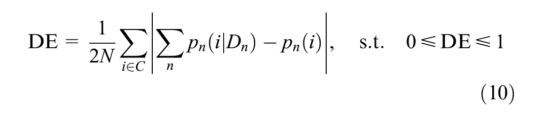
term is taken to prevent the positive and negative massing errors of different alternatives from canceling out. We refer to this metric dispersion error because it measures the degree to which the distribution of aggregate demand for a set of choosers is under- or overdispersed relative to the “true” distribution that is observed when no sampling is performed.

Equation 11 follows from the assumption that when sampling without replacement, $D_{n} = C$ for any $D_{n}$ constructed using a 100% sample.

lim_{\tilde{J_{n}} \to J} p_{n} (i | D_{n}) = p_{n} (i)

(11)

Equation 12 follows from substituting Equation 11 into Equation 10, and shows that dispersion error, DE, should trend toward zero as the size of the sample, $\tilde{J_{n}}$ , approaches $J$ :

lim_{\tilde{J_{n}} \to J} DE = 0

(12)

Thus, by varying the size of $D_{n}$ and measuring the rate at which dispersion error approaches zero, we were able to quantify the marginal benefit of using larger and larger sample rates. We hypothesized that the magnitude of this benefit would depend on both the size of the universe of alternatives, $J$ , and the precision/error of the model itself.

Data Generation

The data generation procedure used in this study builds on that of Nerella and Bhat ( 4 ). We modified both the model specification and the scale of the simulated data to more accurately approximate the form of a location choice model that one might encounter in a modern microsimulation platform like UrbanSim ( 23 ). We describe the changes to the model specification here, and address the scale of the data in the context of the experiment design in the section that follows.

The model is structured as a linear-in-parameters MNL specification with five independent variables and coefficients fixed to one. Values for the first three variables were generated according to the same procedure described in Nerella and Bhat: dividing the alternatives into two subsets and drawing values from the standard univariate normal distribution using a mean value of 1.0 for the first subset and 0.5 for the second ( 4 ). For the fourth variable we introduced an interaction term between an alternative-specific attribute drawn Lognormal(1, 0.5) and a chooser-level attribute drawn Lognormal(0, 0.5). Interaction terms like this are a common feature of location choice models because they capture chooser preference heterogeneity that arises from real-world relationships (e.g., rent-to-income ratio, home-to-work distance). The fifth variable was sampled Lognormal(0, 1) and was meant to approximate a spatial measure like distance to a central business district.

Experiment Design

A series of simulations were performed in which choice probabilities were generated for synthetic datasets while approximating different modeling scenarios along three experimental controls: 1) sample rate $(\frac{\tilde{J_{n}}}{J})$ ; 2) the scale parameter $(μ)$ of the logit model; and 3) the scale of the data (N and J). A total of 1,750 scenarios were modeled using 10 sample rates, 7 scale parameters, and 25 dataset sizes. We computed the dispersion error for each of these to aggregate the results of each scenario over 10 runs for a total of 17,500 simulations.

For each chooser, n, in each dataset we constructed 10 choice sets. The first of these was simply C, the universe of alternatives. The other nine choice sets, $D_{n 1} \dots D_{n 9}$ , were assembled through SRS without replacement from C using nine equally spaced sample rates along the interval from 10% to 90%. To construct each D_ns of size $\tilde{J_{ns}}$ we first partitioned the alternatives in C into 10 random subsets, $S_{n 1} \dots S_{n 10}$ , with $\frac{J}{10}$ elements each. Then, setting $D_{n 1}$ equal to $S_{n 1}$ , we reincorporated the remaining subsets one at a time as follows:

D_{ns} = D_{ns - 1} \cup S_{ns} s = {1, \dots, 9}

(13)

such that $\tilde{J_{ns}} = \frac{J}{10}$ . Although this approach meant that $D_{n 1} \dots D_{n 9}$ were not drawn independently for a given chooser, it reduced the number of times we needed to draw random samples without replacement by a factor of 10. Given that the compute time of the sampling algorithm we used was $O (J + J \log J)$ , this was a necessary compromise to ensure we could simulate over the largest choice sets ( $J = 2 \times 10^{6}$ ) in a reasonable amount of time ( 24 , 25 ). In tests run on smaller choice set sizes, the effect of this design was found to be insignificant with respect to our experimental results.

The scale parameter was the second critical axis of inquiry in this study. Since $μ$ was confounded with the vector of coefficients, $β$ , and all $ϵ_{in}$ s were assumed to be independent and identically distributed, common practice is to simply set $μ = 1$ ( 26 ). In this case, however, we knew a priori that each of the coefficients would be 1. This created a unique opportunity to use $μ$ as an experimental control for model precision. From Equation 1, it follows that as $μ \to 0$ the model becomes completely random with all alternatives having equal probability:

lim_{μ \to 0} p_{n} (i) = \frac{1}{J} \forall i = {1, \dots, J}

(14)

Thus, we expected DE to trend toward zero in this case as well. Conversely, as $μ \to \infty$ , the model becomes completely deterministic, which should produce the highest values of error due sampling of alternative. Thus, to investigate the effect of model precision on dispersion error, we repeated each simulation for seven values of the scale parameter:

μ = {0.25, 0.5, 0.75, 1, 1.25, 1.5, 1.75}

This is analogous to the approaches of Lemp and Kockelman ( 3 ) and Guevara and Ben-Akiva ( 27 ) to assess the effect of noisy data on parameter estimation.

Lastly, we generated 25 synthetic populations of N choosers and J alternatives representing all possible combinations of N and J:

N = {7.5 \times 1 0^{2}, \dots, 7.5 \times 1 0^{6}}, and J = {2 \times 1 0^{2}, \dots, 2 \times 1 0^{6}}

This made it possible to assess the change in DE as the scale of the model approached that of microsimulation in relation to number of choosers and alternatives. All 25 datasets were regenerated for every value of $μ$ for each of the 10 runs for a grand total of 1,750 distinct datasets.

Alternative Sampling Strategies

The final component of the analysis investigated the benefits of alternative sampling strategies over SRS. In theory, a strategic sampling strategy like importance sampling should reduce the sample rate required to obtain choice sets with relevant (i.e., high utility) alternatives. Since the experiment described above necessarily involves computing the true, unconditional choice probabilities, $p_{n} (i)$ , for all choosers and alternatives, we conducted a second set of simulation runs in which each choice set, $D_{ns}$ , was constructed using these probabilities as sample weights. The use of importance sampling means choice sets are no longer constructed from truly random draws. As such, the uniform conditioning property does not hold, and the more generalized form of the conditional probability, $p_{n} (i | D_{n})$ (Equation 1), must be used instead ( 26 ).

Computation

The entirety of each simulation, from sampling of alternatives to the calculation of choice probabilities, was performed on a single NVIDIA GeForce RTX 3090 graphics processing unit (GPU). We leveraged the open source JAX library to perform extremely fast linear algebra operations on the GPU ( 24 ). Although the duration of each simulation was still quite long for the largest datasets (Figure 2), initial tests indicated that run times with a CPU-based approach would have been prohibitively slow. It is possible that massive parallelization across a sufficient number of CPUs could achieve run times comparable to the GPU but such an approach was determined to be cost-prohibitive given the number of processors required and the current cost of on-demand cloud computing resources.

Figure 2.

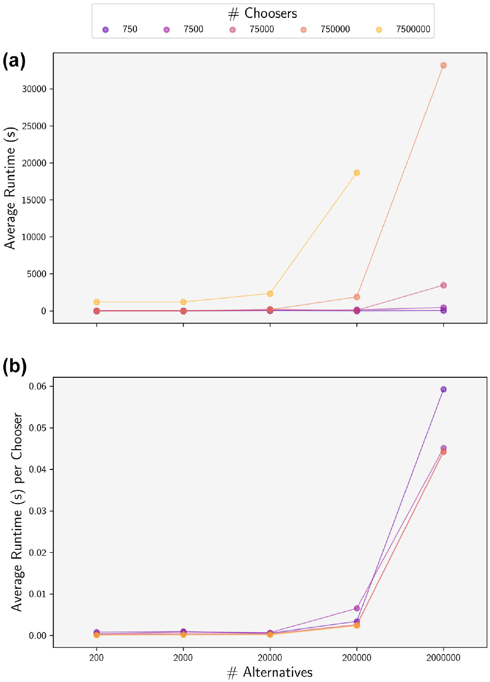
Average runtime: (a) and runtime per chooser (b) for each of the 1,750 datasets by population size (N and J). A single runtime represents the total duration to simulate probabilities and compute dispersion error at all nine sample rates.

The use of a single GPU does impose strict limits on the amount of data that can be processed at once. We experimentally determined that the full table of $N \times J$ probabilities would exceed the 24GB memory capacity of the GPU for scenarios where $N \times J \geq 1.5 \times 10^{9}$ . In scenarios above this threshold, we computed choice probabilities in batches of choosers, with larger datasets requiring more batches, and fewer choosers per batch as J increased. The inefficiency of batched processing is reflected in Figure 2, which shows that the average and per-chooser runtimes were essentially invariant to the number of choosers until the dataset sizes exceeded the batching threshold. This meant that although the analysis was quite slow to run for the largest datasets, runtimes could be drastically reduced by processing batches simultaneously across a cluster of GPUs rather than in a queue on a single processor. However, such optimization was not the intent of this research.

Results

Experimental Results

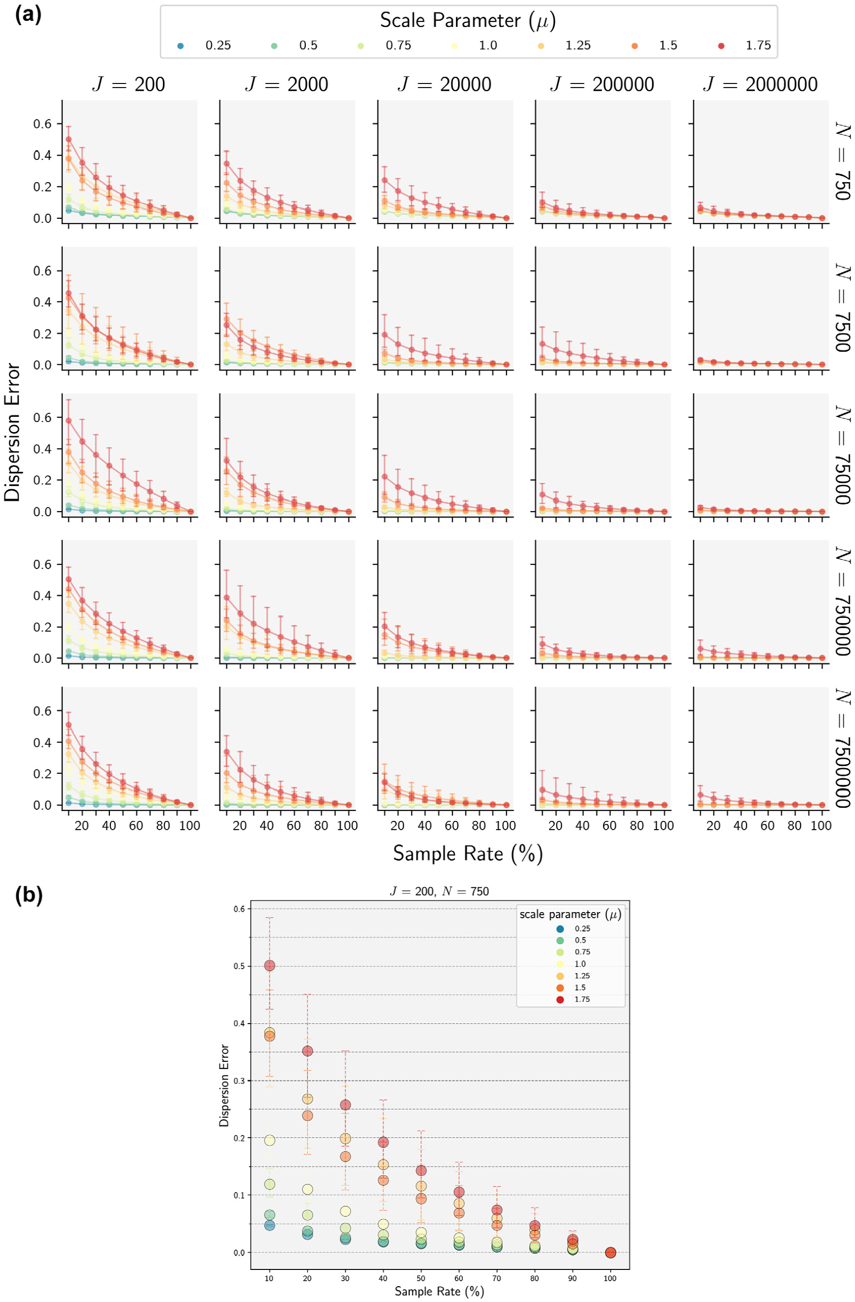
In general we found that dispersion error was highly correlated with lower sample rates, model error ( $μ$ ), and smaller choice sets (J). Figures 3 and 4 highlight these relationships across each of the 25 dataset sizes. The effect of sample rate aligns with expectations, with dispersion error trending toward zero as sample rate approaches 100%. In nearly every case we observe a trend of diminishing benefits for marginal increases in sample rate, with the greatest reduction in dispersion error observed on the interval from 10 to 20%.

Figure 3.

(a) Mean dispersion error across 10 runs for each of the 1,750 model scenarios. Curves highlight the rate at which dispersion error decreases with larger sample rates. (b) Detailed view of the top left grid cell from (a).

Figure 4.

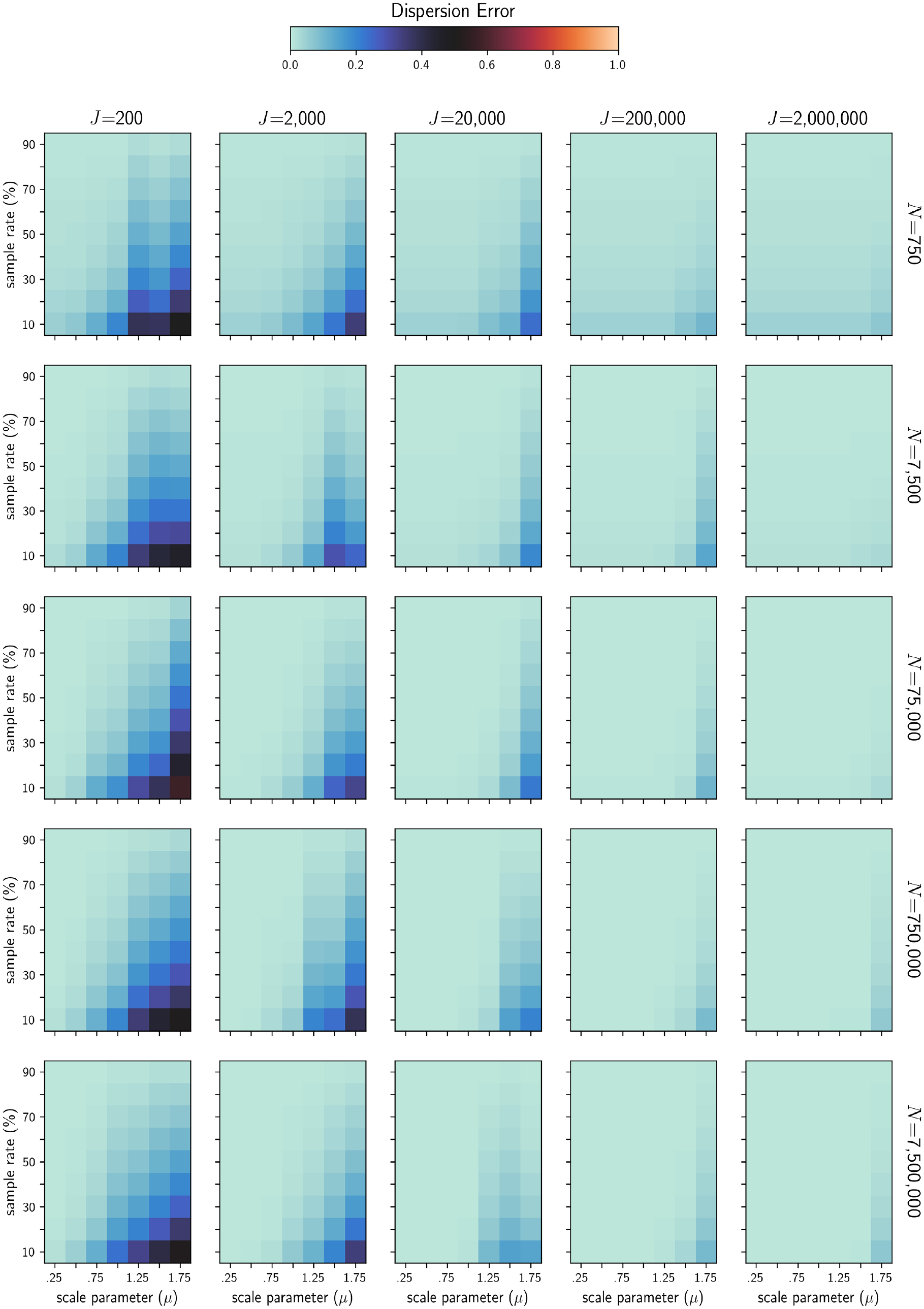
Heatmaps showing differences in mean dispersion error across scenarios.

Lower model precision was consistently associated with lower levels of dispersion error, lending support to the initial hypothesis about the attenuating effect of model noise on error owing to sampling of alternatives. Notably, in several cases the effect of model noise was found to have a greater impact on dispersion error than sample rate. For example, Figure 3b shows that that reducing the precision by a factor of two ( $μ = 1$ to $μ = 0.5$ ) had a greater impact than tripling the sample rate (10% to 30%). Obviously, in practice a modeler does not have the ability to exogenously define or even observe the scale parameter separately from the parameter coefficients, but this finding is nevertheless significant. In particular, it suggests that in low-precision models, there is less to be gained from using larger and larger sample rates.

The size of the universe of alternatives (J) was also observed to have a significant effect on dispersion error, albeit the opposite effect of what was anticipated, with the highest levels of error observed for models with the fewest alternatives, and comparatively little dispersion error observed for scenarios with the largest choice sets. For example, at J = 2e6, the range of dispersion error observed for a 10% sample rate across all values of $μ$ was reduced to that of a 70% to 80% sample for the equivalent J = 200 scenario. Although the cause of this trend was not immediately clear, it did align with results reported by both Lemp and Kockelman ( 3 ) and Nerella and Bhat ( 4 ), though neither paper makes explicit mention of it. This finding is discussed in greater detail in the discussion section below.

Strategic Sampling of Alternatives

The results of the importance sample simulation runs, summarized in Figure 5, showed that the benefit of importance sampling over SRS was limited only to those models with the highest levels of precision (i.e., very low variance of error). 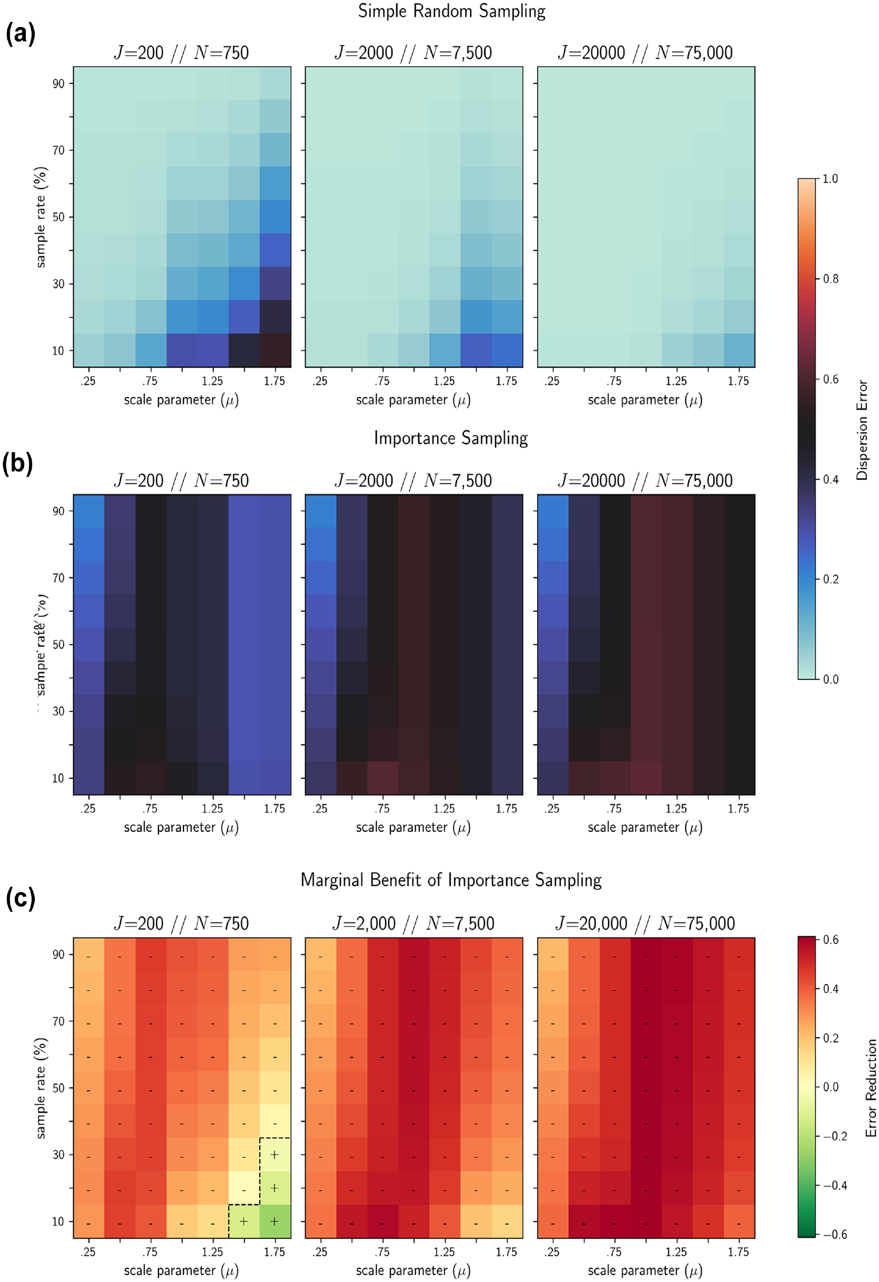More surprisingly, however, was that importance sampling actually performed worse than SRS for the majority of scenarios tested here, particularly for large scenarios ( $J \leq 2000$ ) and low-precision models ( $μ < 1$ ). This represents an important and novel finding of the study, which challenges traditional wisdom about best practices for sampling from large choice sets.

Figure 5.

A comparison of mean dispersion error for 10 runs under (a) simple random sampling (SRS) and (b) importance sampling. Only 4 of the 189 (2.1%) scenarios tested exhibit reduced dispersion error under importance sampling, identified in (c) the heatmaps with a “+”; otherwise, SRS provides a much better fit to the true distribution of aggregate demand.

Figure 6 shows that this finding held true for a more conventional error form as well: root mean squared error (RMSE). As shown in Equation 15, individual error is still computed at the level of the alternative by using the formula for PME (Equation 8), but here the error term is squared,

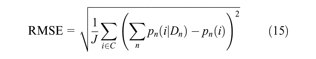
RMSE = \sqrt{\frac{1}{J} \sum_{i \in C} {(\sum_{n} p_{n} (i | D_{n}) - p_{n} (i))}^{2}}

(15)

Aside from being nonlinear, RMSE also differs from dispersion error in that it has no upper bound. This made it difficult to compare RMSE values across scenarios with different numbers of choosers, but still allowed for comparison of different sampling mechanisms for a given scenario. Just like in Figure 5, SRS was shown to outperform importance sampling in all but the smallest, most precise choice scenarios.

Figure 6.

Only four scenarios (indicated by “+”) showed positive reductions in mean root mean squared error (RMSE) when replacing simple random sampling (SRS) of alternatives with an importance sampling approach. In all other cases SRS was found to provide a better fit to the true distribution of aggregate demand. Note that each color gradient has a different range of values, making it difficult to compare results across the three scenarios shown here.

With respect to the size of the universe of alternatives, we found that dispersion error was largely invariant to the scale of J under importance sampling. Meanwhile dispersion error under SRS was shown to decrease dramatically as J increased. Comparatively, this meant that any advantage offered by importance sampling for small J scenarios was quickly lost as the size of the universe of alternatives approached the most disaggregate scales and the performance of SRS improved. The performance of importance sampling was also found to vary with model precision, with the most precise models demonstrating the greatest benefit. This makes intuitive sense, since Equation 5 shows that when $ϵ_{in}$ is smaller, the information contained in the model $V_{in}$ necessarily represents a greater portion of the total utility, $U_{in}$ , for each choice. Although Lemp and Kockelman found a similar correlation between model precision and the benefit of strategic sampling, they were unable to identify this threshold beyond which SRS is able to outperform importance sampling, owing to the limited number of scenarios they tested and their explicit focus on parameter estimation instead of aggregate error ( 3 ).

Less intuitive is why importance sampling would actually exacerbate dispersion error for low-precision models. By examining the individual probability massings (Equation 7) for several scenarios, we were able to determine that the vast majority of this error was actually the result of underdispersion, a kind of statistical overfitting where so much of the aggregate probability mass was allocated to the highest utility alternatives that the lowest probability alternatives were essentially ignored. Figure 7 shows the results of this analysis for a scenario with 750 choosers and 200 alternatives.

Figure 7.

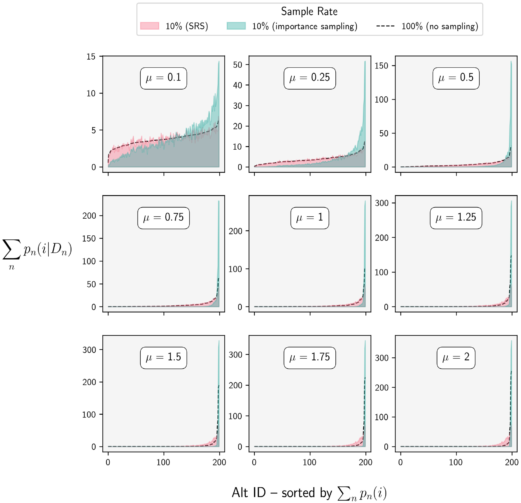
A comparison of the distribution of probability massings (PM_i) for a population of 750 choosers and 200 alternatives generated using a 10% sample rate under two sampling procedures. Importance sampling (turquoise) produced a more accurate distribution of aggregate choice probability when model precision was high ( $μ > 1.25$ ) and the true distribution of probability mass was concentrated among fewer alternatives. Conversely, when model precision was low, importance sampling led to underdispersion of aggregate choice probability relative to the true distribution.

One possible explanation as to why this phenomenon has gone unnoticed until now is that underdispersion does not lead to choosers selecting “bad” alternatives. This means that any metric that relies on the simulated choices of individual choosers, such as those used in the studies by Lemp and Kockelman ( 3 ) and Nerella and Bhat ( 4 ), rather than the full distribution of choice probabilities, cannot capture this type of error.

Application to Real Data

To validate our experimental results, we estimated a location choice model with real data from the 2012 California Household Travel Survey (CHTS). We limited this model to include only in-region, out-of-home discretionary activities completed by residents of the nine-county San Francisco Bay Area during the survey period (n = 28,880). We aggregated activity locations to the census block group (n = 106,910), and estimated a model by randomly sampling 1,000 alternatives per chooser. Given the already extremely small standard errors obtained from this model (Table 1), it was deemed unnecessary to use a larger sample size.

Table 1.

Summary of a Discretionary Location Choice Model Estimated from CHTS Data (n = 28,880)

Description	Coefficient	SE	z
Log(% retail)	2.2708	0.032	71.363
Log(total jobs)	0.6120	0.003	233.446
Log(total population)	0.0377	0.002	15.918
Jobs-to-housing ratio	−0.0001	0.000	−11.055
Log(distance to CBD): household vehicles/person	0.1165	0.001	110.500

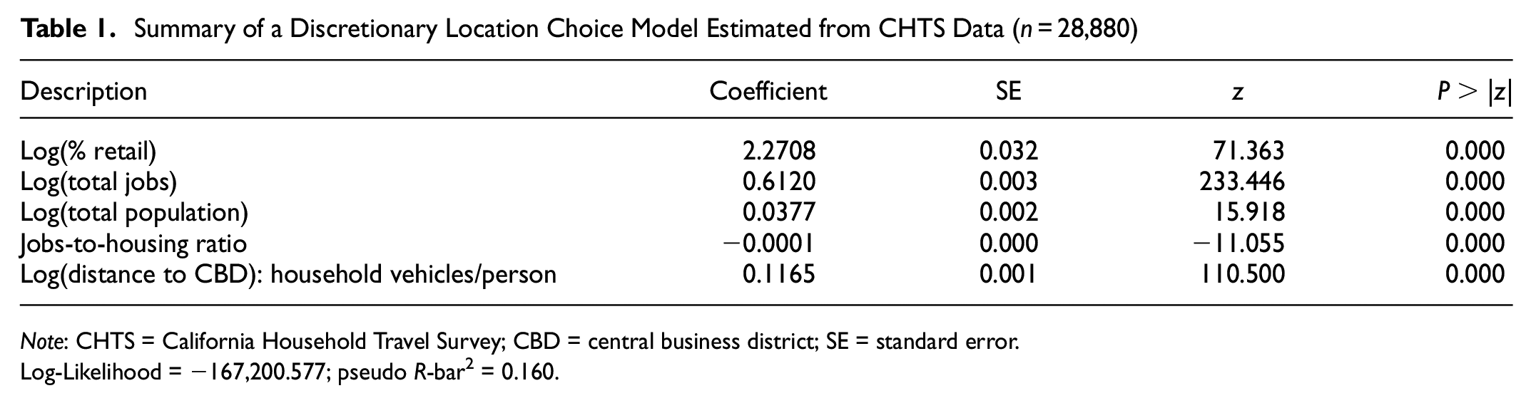
Note: CHTS = California Household Travel Survey; CBD = central business district; SE = standard error.

Log-Likelihood = −167,200.577; pseudo R-bar² = 0.160.

For the prediction phase we generated a synthetic population of choosers using the open source SynthPop software ( 28 ). From this we randomly sampled 4e5 choosers such that the ratio of choosers to alternatives was comparable to that of the original Nerella and Bhat experiment ( 4 ). We then performed the same series of simulations that were carried out on the synthetic data, varying the sample rate and scale parameter (J was fixed), and computed dispersion error for each scenario. 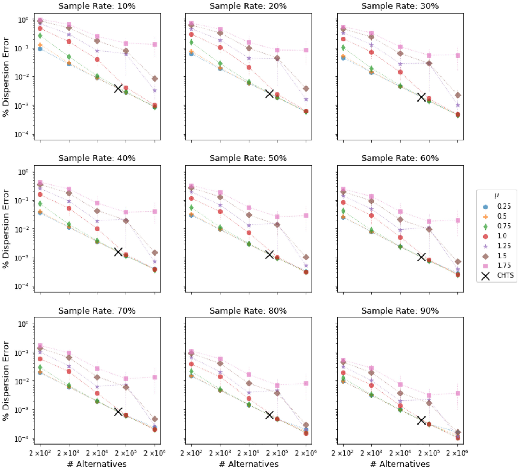A comparison of these results against the experimental data showed that the dispersion error in the CHTS model closely approximated the expected error of the low-precision ( $μ < 1$ ) experimental models for a similarly sized dataset (Figure 8). This pattern held true for all nine sample rates, and suggests that the experimental findings described above were more than an artifact of the data generation process. Importantly, it also provided contextual information about the relative precision of the CHTS model insofar as it related to prediction error. We discuss the significance of this below.

Figure 8.

A comparison of experimental results to those obtained from a model estimated on data from the California Household Travel Survey (CHTS). Each grid cell plots the relationship between average dispersion error and the size of the universe of alternatives for a given scale parameter ( $μ$ ) and sample rate. The black “X” represents the CHTS results in which the true scale parameter is unknown.

Discussion

The results of this analysis raises several critical issues that, to date, have not been adequately addressed in the scientific literature on sampling of alternatives in discrete choice models. We briefly describe each of these here, and discuss their implications both for practitioners and future research.

The Inadequacy of Sample Rate Recommendations

The first two issues arise from the observation that in several scenarios, both model precision and the size of the universe of alternatives were found to be more significant determinants of the bounds of dispersion error than sample rate alone. This suggests that the validity of several commonly cited sample rate guidelines may be more limited than previously thought. For example, Nerella and Bhat recommend a minimum sample rate of one-eighth for MNL using SRS ( 4 ). They do not, however, test the robustness of this result against varying levels of model precision, making it impossible to determine how well their findings might generalize to a model estimated on real data. Furthermore, their findings are based on experiments in which the total number of alternatives is fixed to 200, which, given the evidence presented here, would likely not hold for choice scenarios in which the universe of alternatives is many orders of magnitude larger, such as those found in even modestly disaggregate travel or land use demand models. The good news for practitioners is that larger choice scenarios are associated with smaller aggregate error from sampling of alternatives and thus the sample rate recommended by Nerella and Bhat is probably much larger than necessary, particularly for the most disaggregate scenarios ( 4 ). This was made clear from Figure 8, which shows that average dispersion error is reduced by approximately two orders of magnitude as the size of the universe of alternatives increases from 2e2 to 2e6, regardless of the scale parameter and sample rate.

The sensitivity of dispersion error to model precision is particularly problematic for establishing sampling guidelines because, in practice, one cannot explicitly observe the scale parameter separately from the estimated parameters. However, the simulation results from the CHTS model described above make it possible to infer something about the expected range of precision one might encounter in the real world. Specifically, Figure 8 shows that the dispersion error observed in the CHTS model aligns quite nicely with the experimental results for models in the low-precision regime ( $μ < 1$ ). This is a strong indication that the CHTS model, and other highly disaggregate location choice models like it, may have relatively low levels of precision. If this is the case, then based on evidence presented here, practitioners should expect only modest gains from the use of sample rates greater than 10% under SRS (Figures 3 and 4). This is consistent with what we observed in the CHTS model, in which dispersion error decreased from ∼0.004 to ∼.0025 when doubling the sample rate from 10% to 20%. A ∼40% reduction in error might seem significant, but in absolute terms it corresponds to a mere 0.15% of the total probability mass of the population. More work should be done to confirm these findings using other sources of estimation data and simulated choices.

Compared with model precision, that the size of the universe of alternatives is a known quantity should make it easier for practitioners to incorporate its observed effect into their modeling decisions. However, given the surprising finding that large J scenarios actually exhibited less overdispersion as a proportion of total probability mass, some additional discussion is merited. Figure 9 shows the results of a secondary analysis in which we compared the empirical distribution of true probability massings for two different values of J. These results show that as J increased, the aggregate choice probabilities became more concentrated in the peak and tails of the distribution, as measured by higher values of skewness and kurtosis, respectively. However, both the standard deviation and the maximum value of probability mass for a given alternative were on average smaller. 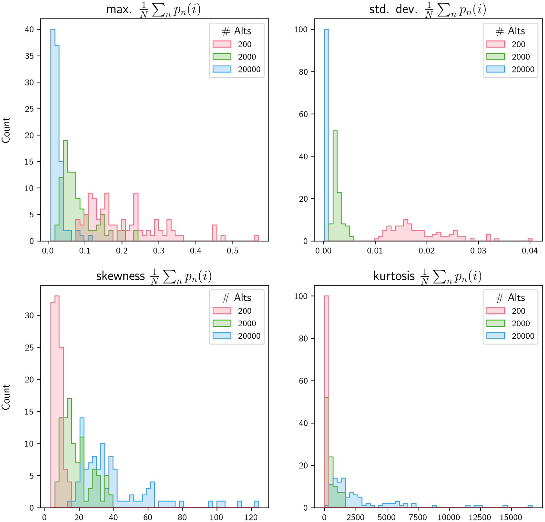The net effect of these dynamics was that the peak of the distribution of $\frac{1}{N} \sum_{n} p_{n} (i)$ did not grow as fast as the tail, meaning that the number of bad alternatives increased faster than the aggregate probability that was concentrated in the good ones. In one sense, then, the initial hypothesis about the effect of J was correct: as the size of the universe of alternatives increases, SRS is less likely to produce choice sets containing the highest probability alternatives. So why then does error resulting from random sampling of alternatives actually improve for larger values of J ?

Figure 9.

Descriptive statistics of the true distribution of probability mass by number of alternatives, J, for 100 iterations with $μ = 1$ .

To answer this question, one must recognize that the goals of model estimation and forecasting are not the same. Specifically, in a choice scenario where alternatives are not subject to capacity constraints, forecast performance is not optimized by increasing the within-sample variance among alternatives like it is for estimation. Rather, if the accuracy of a forecast under sampling of alternatives is defined by the ability to replicate the aggregate demand for alternatives obtained without sampling alternatives, it follows that optimal results are obtained when sampled choice sets are representative of the universe of alternatives. Thus, if the variance of $\frac{1}{N} \sum_{n} p_{n} (i)$ shrinks for larger values of J, dispersion error resulting from random sampling of alternatives should decrease as well. It is also worth noting that even though we have artificially controlled for model precision in this secondary analysis, in practice precision will be strongly correlated with the variance of the utility of alternatives. This idea is supported by the results of the CHTS model, which showed that a typical microsimulation-scale location choice model belongs to the regime of low-precision models in which dispersion error is relatively small.

Simple Random Sampling: Not So Bad After All?

The distinction between estimation and forecasting also explains why the widely held belief about the benefit of importance sampling proved incorrect in the context of this study. As shown in Figure 7, importance sampling did in fact produce distributions of aggregate demand where a greater proportion of probability mass was allocated to the higher utility alternatives. Since the utility functions themselves were unchanged between the sampling strategies, this simply meant that importance sampling was functioning as intended, with high-utility alternatives showing up in sampled choice sets more frequently. This is what makes importance sampling beneficial for parameter estimation. However, the results shown here suggest that in the context of forecasting aggregate demand for alternatives that are not capacity constrained (e.g., discretionary activity location or route choice), this very same mechanism could actually lead to dispersion error of another kind: underdispersion, or an overallocation of probability mass to high-utility alternatives. Importantly, this result was shown to hold true using RMSE, a more traditional measure of model error. For choice scenarios that are capacity constrained (e.g., building-level residential location choice), or models that treat demand as a market-clearing process, over-selection of high-probability alternatives is not possible and the effect of this underdispersion is likely immaterial. However, in the absence of capacity constraints, importance sampling may in fact produce demand forecasts that are less accurate than what would be obtained with SRS, particularly if model precision is low or the size of the universe of alternatives is large. It is possible that a less precise importance sampling approach, one that is not based on the true probabilities, $p_{n} (i)$ , for each alternative, would mitigate this effect. Future work should investigate whether heuristic-based importance sampling strategies, for example one based on the distribution of observed trip distances, might perform better.

Conclusions

The results of this study strongly suggest that forecast error resulting from sampling of alternatives in discrete choice models is less significant than previously hypothesized. In several cases, SRS was shown to produce choice probabilities that matched the true distribution of aggregate demand quite well, particularly when model precision was low. Since model precision was expected to decrease as the size of the universe of alternatives increased, it follows that the impact of random sampling of alternatives should lessen as choice scenarios approach the microsimulation scale. Empirical evidence from a model estimated on real survey data lent further credibility to the notion that microsimulation-scale models tend to have low levels of precision relative to the wide range of scenarios tested here. Additionally, SRS was found to outperform an importance sampling strategy for all but the smallest, most precise choice scenarios. This result held true using both the novel measure of forecast error present here as well as more traditional error measures like RMSE. Although the validity of this finding was limited to unconstrained choice problems, it is nonetheless significant in that it challenges the prevailing belief that optimal sampling strategies for model estimation are necessarily optimal for simulation as well.

A secondary contribution of this study is that it has demonstrated the potential of GPU-based computing for simulation of discrete choice models with massive choice sets. It is quite possible that as GPU technology becomes more pervasive (and less expensive), sampling of alternatives may no longer be necessary at all. In the meantime, land use and travel demand modelers would do well to mind the differences between estimation and forecasting as it relates to sampling of alternatives, and think twice before assuming that importance sampling will improve model performance.

Footnotes

Acknowledgements

The authors wish to thank Angelo Guevara and Joan Walker whose expert guidance made this study possible.

Author Contributions

The authors confirm contribution to the paper as follows: study conception and design: M. Gardner, P. Waddell; data collection: M. Gardner; analysis and interpretation of results: M. Gardner, P. Waddell; draft manuscript preparation: M. Gardner. All authors reviewed the results and approved the final version of the manuscript.

Declaration of Conflicting Interests

The authors declared no potential conflicts of interest with respect to the research, authorship, and/or publication of this article.

Funding

The authors received no financial support for the research, authorship, and/or publication of this article.

ORCID iDs

Max Gardner

Paul Waddell

References

Lemp

J. D.

McWethy

L. B.

Kockelman

K. M.

From Aggregate Methods to Microsimulation: Assessing Benefits of Microscopic Activity-Based Models of Travel Demand. Transportation Research Record: Journal of the Transportation Research Board, 2007. 1994: 80–88.

Wegener

From Macro to Micro—How Much Micro Is Too Much?

Transport Reviews, Vol. 31, No. 2, 2011, pp. 161–177.

Lemp

J. D.

Kockelman

K. M.

Strategic Sampling for Large Choice Sets in Estimation and Application. Transportation Research Part A: Policy and Practice, Vol. 46, 2012, pp. 602–613.

Nerella

Bhat

C. R.

Numerical Analysis of Effect of Sampling of Alternatives in Discrete Choice Models. Transportation Research Record: Journal of the Transportation Research Board, 2004. 1894: 11–19.

Zeng

Zhong

Hunt

J. D.

Analysis of the Impact of Sample Size, Attribute Variance and Within-Sample Choice Distribution on the Estimation Accuracy of Multinomial Logit Models Using Simulated Data. Journal of Systems Science and Systems Engineering, Vol. 27, No. 6, 2018, pp. 771–789.

McFadden

Modeling the Choice of Residential Location. Transportation Research Record: Journal of the Transportation Research Board, 1978. 673: 75–76.

Koppelman

F. S.

Chu

Effect of Sample Size on Disaggregate Choice Model Estimation and Prediction. Transportation Research Record: Journal of the Transportation Research Board, 1983. 944: 60–69.

Ben-Akiva

Watanatada

Application of a Continuous Spatial Choice Logit Model. In Structural Analysis of Discrete Data with Econometric Applications ( Manski

C. F.

McFadden

, eds.), MIT Press, London, 1981, pp. 320–343.

Frejinger

Bierlaire

Ben-Akiva

Sampling of Alternatives for Route Choice Modeling. Transportation Research Part B: Methodological, Vol. 43, No. 10, 2009, pp. 984–994.

10.

M. T.

Chow

L. F.

Zhao

S. C.

Geographically Stratified Importance Sampling for the Calibration of Aggregated Destination Choice Models for Trip Distribution. Transportation Research Record: Journal of the Transportation Research Board, 2005. 1935: 85–92.

11.

Train

K. E.

McFadden

D. L.

Ben-Akiva

The Demand for Local Telephone Service: A Fully Discrete Model of Residential Calling Patterns and Service Choices. The RAND Journal of Economics, Vol. 18, No. 1, 1987, pp. 109–123.

12.

Hassan

M. N.

Rashidi

T. H.

Nassir

Consideration of Different Travel Strategies and Choice Set Sizes in Transit Path Choice Modelling. Transportation, Vol. 48, No. 2, 2021, pp. 723–746.

13.

Curtis-Ham

Bernasco

Medvedev

O. N.

Polaschek

D. L.

The Importance of Importance Sampling: Exploring Methods of Sampling from Alternatives in Discrete Choice Models of Crime Location Choice. Journal of Quantitative Criminology, Vol. 38, 2022, pp. 1003–1031.

14.

Castiglione

Freedman

Bradley

Systematic Investigation of Variability Due to Random Simulation Error in an Activity-Based Microsimulation Forecasting Model. Transportation Research Record: Journal of the Transportation Research Board, 2003. 1831: 76–88.

15.

Eliasson

The Influence of Accessibility on Residential Location. In Residential Location Choice ( Pagliara

Preston

Simmonds

, eds.), Springer, Berlin, Heidelberg, 2010, pp. 137–164.

16.

Waddell

Borning

Noth

Freier

Becke

Ulfarsson

Microsimulation of Urban Development and Location Choices: Design and Implementation of UrbanSim. Networks and Spatial Economics, Vol. 3, No. 1, 2003, pp. 43–67.

17.

Jones

Thomas

Peeters

Forecasting Jobs Location Choices by Discrete Choice Models: A Sensitivity Analysis to Scale and Implications for LUTI Models. Region, Vol. 2, No. 1, 2015, pp. 67–93.

18.

Guevara

C. A.

Ben-Akiva

M. E.

Change of Scale and Forecasting with the Control-Function Method in Logit Models. Transportation Science, Vol. 46, No. 3, 2012, pp. 425–437.

19.

Orcutt

G. H.

Caldwell

Wertheimer

Policy Exploration Through Microanalytic Simulation. The Urban Insitute, Washington, D.C., 1976.

20.

Walker

J. L.

Making Household Microsimulation of Travel and Activities Accessible to Planners. Transportation Research Record: Journal of the Transportation Research Board, 2005. 1931: 38–48.

21.

Koehler

Brown

Haneuse

S. J. P.

On the Assessment of Monte Carlo Error in Simulation-Based Statistical Analyses. The American Statistician, Vol. 63, No. 2, 2009, pp. 155–162.

22.

Wang

Waddell

Outwater

Incremental Integration of Land Use and Activity-Based Travel Modeling: Workplace Choices and Travel Demand. Transportation Research Record: Journal of the Transportation Research Board, 2011. 2255: 1–10.

23.

Waddell

UrbanSim: Modeling Urban Development for Land Use, Transportation, and Environmental Planning. Journal of the American Planning Association, Vol. 68, No. 3, 2002, pp. 297–314.

24.

Bradbury

Frostig

Hawkins

Johnson

M. J.

Leary

Maclaurin

Necula

, et al. JAX: Composable Transformations of Python+NumPy Programs. 2018. http://github.com/google/jax.

25.

Veira

Algorithms for Sampling Without Replacement — Graduate Descent. 2019. https://timvieira.github.io/blog/post/2019/09/16/algorithms-for-sampling-without-replacement/. Accessed March 11, 2022.

26.

Ben-Akiva

M. E.

Lerman

S. R.

Discrete Choice Analysis: Theory and Application to Travel Demand, Vol. 9. MIT Press, Cambridge, MA, London, 1985.

27.

Guevara

C. A.

Ben-Akiva

M. E.

Sampling of Alternatives in Logit Mixture Models. Transportation Research Part B: Methodological, Vol. 58, 2013, pp. 185–198.

28.

Konduri

Pendyala

R. M.

Sana

Waddell

A Methodology to Match Distributions of Both Household and Person Attributes in the Generation of Synthetic Populations. Presented at 88th Annual Meeting of the Transportation Research Board, Washington, D.C., 2009.

Numerical Analysis of Error From Sampling of Alternatives in Logit-Based Demand Forecasting Models with Massive Choice Sets

Abstract

Keywords

Background

Key Questions and Contributions of this Study

Methodology

Measuring Dispersion Error

Data Generation

Experiment Design

Alternative Sampling Strategies

Computation

Results

Experimental Results

Strategic Sampling of Alternatives

Application to Real Data

Discussion

The Inadequacy of Sample Rate Recommendations

Simple Random Sampling: Not So Bad After All?

Conclusions

Footnotes

Acknowledgements

Author Contributions

Declaration of Conflicting Interests

Funding

ORCID iDs

References