Sage Journals: Discover world-class research

Abstract

The emerging connected and automated vehicle (CAV) technology is likely to bring significant changes to the transportation world. This study helps understand how the anticipated emergence of CAVs will affect various aspects of society and transportation, including travel demand, vehicle miles traveled, energy consumption, and emissions of greenhouse gases and other pollutants. We design a set of future system configurations under the California Statewide Travel Demand Model framework to simulate scenarios for the deployment of passenger CAVs in California by 2050. These scenarios consider the ownership and operational type (e.g., private and shared) of CAVs, as well as additional policies such as pricing and the use of zero-emission vehicles (ZEVs) to curb potential impacts. The scenarios are: 0. Baseline (no automation); 1. Private CAV; 2. Private CAV + Pricing; 3. Private CAV + ZEV; 4. Shared CAV; 5. Shared CAV + Pricing; 6. Shared CAV + ZEV. Impacts of the introduction of CAVs across the transportation system are quantitatively estimated. The results indicate that the mode shares of public transit and in-state air travel will likely sharply decrease, while total vehicle miles traveled (VMT) and emissions will likely increase, because of the relative convenience of CAVs. The results also show that VMT could be substantially affected by a modification in auto travel costs. This means that the implementation of pricing strategies and congestion pricing policies, together with policies that support the deployment of shared and electric CAVs, could help reduce tailpipe pollutant emissions in future scenarios.

Keywords

connected and automated vehicles travel demand forecasting travel behavior transportation and sustainability

Automated driving technologies have made great strides forward and might be commercially available in the near future. Progress in the field of self-driving vehicles has the potential to substantially affect travel demand, with eventual large impacts on vehicle miles traveled (VMT), energy consumption, and greenhouse gas (GHG) and criteria pollutant emissions. Further, connected and automated vehicles (CAVs) could substantially modify the existing transportation systems by integrating with other on-demand mobility services and zero-emission fuels, leading to different outcomes depending on the way this technology is brought to the market and the policies that are enacted to regulate the field. Understanding the extent of these impacts is crucial and timely for policymakers and transportation professionals.

To date, a wide range of possible effects of the deployment of CAVs have been estimated based on a variety of datasets, modeling assumptions, and hypothetical scenarios. Particularly, the California Department of Motor Vehicles and the California Public Utility Commission have approved driverless vehicles and on-demand passenger testing and services (including Waymo, Tesla, Lyft, and other automotive, and ride sharing companies) in California. However, limited attention has been given to evaluating the potential impacts on energy consumption, air quality, and criteria pollutant and GHG emissions. Thus, this research studies the future transportation scenarios related to the adoption of CAVs in California. Space limitations mean that we only highlight the factors that are directly related to travel demand modeling and group the impacts into three larger groups (see Table 1), which further include the impacts of CAVs on transportation supply, transportation demand and travel behavior, land use and urban design, environment, and equity.

Table 1.

Potential Impacts of Connected and Automated Vehicles

Category	Change and uncertainty	Direct implications	Indirect implications
Transportation supply	Advanced vehicle technology	Vehicle operating cost Safety	• Vehicle miles traveled • Energy consumption • Air pollution • Activity pattern • Social equity
Transportation supply	Improved traffic flow	Capacity Congestion
Travel demand and behavior	Travel cost	Monetary cost Travel time Value of time
	Mode choice	Mode share
	Long-distance travel	Trip generation Mode share
	Vehicle ownership	Mode share
	Mobility	Sharing Mobility for the population with limitations
Land use	Parking	Travel cost
	Location choice	Home-based origin Destination choice
	Accessibility	Mode share

There is no doubt about the potential changes that will occur in transportation supply when automated vehicles (AVs) become available. With sufficient penetration rate and connectivity, CAVs will likely improve traffic flow. Improved traffic throughput is viewed as an achievable goal through vehicle automation. Evidence from several studies suggests that automated systems will be able to improve traffic ﬂow in the future with sufficient penetration rate and vehicle cooperation. One of the main contributors to the changes in transportation supply can be the success of implementing various vehicle control strategies, a central component of automated driving tasks ( 1 – 4 ). For a CAV to drive smoothly and safely, two decoupled tasks need to be performed simultaneously: (i) controlling the speed to maintain safe headway; (ii) steering to adjust lateral motions of the vehicle. The breakthroughs in vehicle-level control technologies, such as adaptive cruise control and cooperative adaptive cruise control (CACC), show the potential benefits of incorporating automation into the highway system ( 5 , 6 ). Advanced control, vehicle technologies, and infrastructure support are likely to result in significant improvements in highway capacity. A pioneer study showed that the highway capacity can increase up to 100% from 2,000 to 4,000 vehicles per hour per lane, with the enhancement offered by vehicle awareness devices and CACC ( 7 ). Throughput improvement with various combinations of AVs and connected vehicles was thoroughly studied by Talebpour and Mahmassani ( 8 ). They found that advanced technologies have the potential to improve the throughput by more than 100%. A more optimistic result shows that 300% improvement of lane capacity is achievable if all vehicles are cooperatively automated ( 9 ). It is also worth noting that there could be different capacity improvement for different roadway or facility types. For example, 40% capacity increase can be achieved at 100% penetration rate for protected movements at signalized intersections ( 10 ). At freeway weaves, up to 11% capacity increases can be achieved compared with Highway Capacity Manual estimates, equipped with the proposed control mechanism ( 11 ). There is still an ongoing research question about the impact on traffic flow of the introduction of CAV in the real world, especially for the mixed traffic flow case, given the projected mass market availability of vehicles that are fully connected and automated that is still on track for the future.

The impacts of CAVs on travel demand and behavior have received considerable attention from researchers who wanted to quantify the impacts of CAVs on the way people travel and engage in activities as well as on the transportation system in general. AVs can change both the fixed out-of-pocket costs of car ownership and the variable transportation costs which are usually defined as distance-based costs ( 12 , 13 ). Another important component is travel time, which includes in-vehicle travel time and out-of-vehicle travel time. It is expected that the value of in-vehicle time will decrease as travelers perceive a reduced burden of travel from no longer needing to drive and being able to engage in activities for purposes other than driving ( 14 , 15 ). On the other hand, we expect that out-of-vehicle time may change because of automation. For example, AVs may reduce walk access/egress time if they are allowed to park by themselves after dropping off the passenger. In the case of the use of SAV (shared CAV), a range of waiting times may add to out-of-vehicle time. For mode choices, the ability to integrate productive activities into commuting trips will affect the value of travel time and mode choice, leading to a potential AV future with much increased use of drive alone modes, at the expense of public transportation and rail modes in particular ( 16 ). Reducing parking costs can have higher impacts on modal split compared with the changes in road capacity and value of time VOT ( 17 ). It is shown that automation can lead to a 3.4% increase in car mode share and a 6% decrease in number of trips by public transit ( 18 ). Americans would expect long-distance travel to shift toward AVs and SAVs, where 50% of the trips between 50 and 500 miles are expected to take place in an AV or SAVs ( 19 ).

For vehicle ownership, privately-owned AVs may still be the most preferable option to consumers, despite a sharp decrease in the per-mile cost of SAVs. One study showed that among the 347 respondents, only 13% indicated they may be willing to give up personal vehicles and rely exclusively on SAVs with the cost of $1/mile ( 20 ). In another study, more than 70% of respondents choose not to use the SAV system ( 21 ). This was also confirmed in another stated preference study where the authors found that only 5.4% of 1,920 respondents from a survey in North America were willing to use SAVs for commuting purposes and only 40.63% were willing to participate in the SAV program (even at zero membership cost) ( 22 ). CAVs are also expected to bring health benefits through reduced traffic incidents and emissions ( 23 ). Besides, CAVs are very likely to affect the built environment ( 24 , 25 ) and improve mobility and accessibility for children, elderly people, and individuals with physical disabilities or other impairments to driving ( 26 ) and the environment ( 27 , 28 ).

A large body of studies have estimated how VMT could change with the future emergence of CAVs. It is worth noting that the results often depend on the data and assumptions used for modeling VMT, as most of these studies are based on modeling simulations rather than on the analysis of travel behavior data and the causes of changes in travel choices. In Table 2 we summarize the findings of some of these studies, the majority of which are based on simulation and the use of a trip-based model or an activity-based model.

Table 2.

Summary of Modeling Practice

Study	Area and types of model	Research questions	Assumptions	Main findings
Fagnant and Kockelman ( 29 )	A hypothetical grid-like city; Agent-based model	Find the impacts of different SAV relocation strategies. Investigate the potential impacts of SAVs on vehicle ownership, VMT, and environment.	• Changes in trip generation (double, half, quarter) • Centralization of trip (more centralized, less centralized) • Service area (greater versus smaller area) • Return-home trip by SAV • Peak congestion • SAV demand (greater morning and evening peak) • Relocation strategies • Limiting number of SAVs	• Each SAV can replace 10–11 conventional cars, serving 31–41 travelers per day with average waiting time of 20 minutes. • VMT can be increased by 4.9% to 10.7%.
Gucwa ( 30 )	San Francisco, CA; Activity-based model (MTC ABM)	Finding the magnitude of the effect from the reduced generalized cost of travel (in mode choice).	+100% road capacity	+2% VMT
			−100% VOT for private AVs	+13% VMT
			+10% to 100% road capacity and −25% to 100% VOT	+4% to 15% VMT
Childress et al. ( 17 )	Seattle, WA; Activity-based model (PSRC SoundCast)	Finding the range of behavioral impacts from AVs (mode and trip-choice model capacity changes for freeways and major arterials).	30% road capacity (all freeway and major arterials)	+4% VMT, −4% VHT
			+30% road capacity and −35% VOT	+5% VMT, −2% VHT
			+30% road capacity and -35% VOT and −50% parking cost	+20% VMT, 17% VHT, −0.3% in PT share, −1.6% in walk share
			SAVs with the cost of $1.65/mile	+35% VMT, −41% VHT, +4% in PT share, +5% in walk share
Zhang et al. ( 31 )	Hypothetical city (10 * 10-mile city with grid-like network); Agent-based model	Understanding the impacts of SAVs on urban parking for various fleet sizes and passenger wait times.	2% of trips with SAVs	−90% parking demand
Fagnant et al. ( 32 )	Austin, TX; Agent-based model (MATSim)	Exploring the impact of SAVs at lower market penetration.	Replace 1.3% of regional trips	One SAV can replace nine conventional vehicles, +8% VMT
Levin and Boyles ( 33 )	Downtown Austin, TX; Multi-class (VOT-based) four-step model	Exploring the impact of AVs on trip, mode, and route choice.	Various parking prices	Transit ridership decreases by 61.4%, AV demand reaches 83% of total personal vehicle demand
Boesch et al. ( 34 )	Zurich, Switzerland; Agent-based model (MATSim)	Exploring the fleet size required for serving different levels of demand.	Replace all private vehicle trips by SAVs	−90% of vehicles
Chen et al. ( 35 )	Hypothetical city (based on Austin, TX); Discrete-time agent-based model	Exploring the management of fleet of electric SAVs.	10% of trips served by SAVs	+7% empty VMT, −87% vehicles
Chen et al. ( 35 )		Exploring the management of fleet of electric SAVs.	10% of trips served by electric SAVs (with recharge time and vehicle range)	+7% to +14% empty VMT; −85% to −73% vehicles
De Almeida Correia and van Arem ( 18 )	Delft, The Netherlands; Traffic assignment	Exploring the impact of replacing privately-owned conventional vehicles with AVs on traffic delays and parking demand.	Replacement of private vehicles with private AVs in households	+17% VMT, +3% in car share, −5.9% in PT trips
			Replacement of private vehicles with private AVs in households, free parking everywhere	20% VMT, +7.8% in car share, −14% in PT trips
			Replacement of private vehicles with private AVs in households, −50% VOT	49% VMT, +9% in car share, −21% in PT trips
Meyer et al. ( 36 )	Switzerland; Travel demand model (macroscopic)	Investigating the changes in accessibility provided by deployment of AVs and SAVs.	+80% road capacity outside urban areas, +40% in urban areas (private AVs)	Minor gains in accessibility for rural municipalities, no change/small decrease in larger cities
Meyer et al. ( 36 )	Switzerland; Travel demand model (macroscopic)		+80% road capacity outside urban areas, +40% in in urban areas (SAVs)	Moderate accessibility gains in rural municipalities, decrease in larger agglomerations
Liu et al. ( 37 )	Austin, TX; Agent-based model (MATSim)	Exploring the impact of the operation of SAVs on travel mode choice.	−50% VOT, $ 0.5/mile operating costs for SAVs	50.9% SAV mode share, +9.8% empty VMT; SAV fleet = 17% of travelers
			−50% VOT, $ 0.75/mile operating costs for SAVs	12.9% SAV mode share, +13.2% empty VMT; SAV fleet = 15% of travelers.
			−50% VOT, $1/mile operating costs for SAVs	10.5% SAV mode share, +15.7% empty VMT; SAV fleet = 13% of travelers
			−50% VOT, $1.25/mile operating costs for SAVs	9.2% SAV mode share, +15.1% empty VMT; SAV fleet = 13% of travelers
Zhang and Guhathakurta ( 38 )	Atlanta, GA; Agent-based model (with discrete event simulator)	Examining the impact of SAVs on urban parking.	5% of market penetration, −100% parking cost, $ 0.5/minute operating costs (car sharing) and $ 0.3/minute (ride sharing)	−4.5% in parking land
Auld et al. ( 39 )	Chicago, USA; Activity-based model (POLARIS)	Exploring the behavioral and operational effect of connected vehicles and AVs.	+12% to 77% road capacity	+1% to +4% VMT
			−25% to −75% VOT, 20% market share of private AVs	+2% to +18% VMT
			−25% to −75% VOT, 75% market share of private AVs	+10% to +59% VMT
			+3% road capacity, −25% VOT, 20% market share of private AVs	+2.7% in VMT
			+77% road capacity, −75% VOT, 100% market share of private AVs	+79% in VMT
Kröger et al. ( 40 )	Germany and USA; Spatial travel demand model	How different contexts can lead to different AV impacts.	−25% VOT for private AVs (7.5% market share)	+3.4% in VKT, +1.3% in car share, −0.2% in PT share
			−25% VOT for private AVs (29.3% market share)	+8.6% in VKT, +3.8 in car share, −0.4% in PT share
			−25% VOT for private AVs (10.1% market share)	+2.4% in VKT, +1% in car share, −0.3% in PT share
			−25% VOT for private AVs (37.6% market share)	+8.6% in VKT, +3.7% in car share, −0.9% in PT share
Zhang et al. ( 41 )	Atlanta, GA; Activity-based model	Understanding the potential for reduction in vehicle ownership through AVs	Replacement of private vehicles with private AVs in households determined by minimum number of AVs to satisfy travel demand of household members.	+13.3% empty VMT, −9.5% vehicles
Zhang and Guhathakurta ( 42 )	Atlanta, GA; Agent-based model + residential location choice model	Examining the potential changes in residential location choice provided by AVs	• AV is not serving other household member when the current trip departs • There is sufficient time for AV to relocate from its location to the origin of the upcoming trip • The potential relocation time is obtained using Google Maps Distance Matrix API service.	(i) More than 18% of the households can reduce vehicles, while maintaining their current travel patterns. (ii) 29.8 unoccupied VMT will be induced per day per reduced vehicles.
Rodier et al. ( 43 )	San Francisco, CA; Activity-based model	Evaluating system-level traffic effects in San Francisco Bay Area	+100% market penetration, +100% roadway capacity	+1% in drive alone, +8% in transit, −5% in active mode, 14% VMT
			+100% market penetration, −25% VOT	+1% in drive alone, −5% in transit, −4% in active mode, 3% VMT
			+100% market penetration, reduced cost per mile from 17.9 cents to 14 cents	+1% in drive alone, −4% in transit, −4% in active mode, 3% VMT
			+100% market penetration, relaxed age restriction between 16 and 13 years old	+6% in drive alone, −12% in transit, −4% in active mode, 2% VMT
Nadafianshahamabadi et al. ( 44 )	Albuquerque, New Mexico; Integrated land use and travel demand model	Impacts of the adoption of AVs on travel demand, congestion and vehicle emissions.	Changes in land use and travel demand	AVs are likely to increase demand and greenhouse gas emissions. For high AV impact scenario, VMT and average trip distances increase by 11% and 12%, respectively. Results are sensitive to change in travel time.
Sonnleitner et al. ( 45 )	Stuttgart region, Germany; an activity chain based model with an integrated destination and mode choice	Integrating AV into four-step models.	Extend macroscopic assignment models to include changes in traffic flow performance caused by AV. Include a differing perception of travel time in macroscopic travel demand models.	First-generation AVs may decrease traffic performance. More developed AVs will improve performance on some parts of the network.

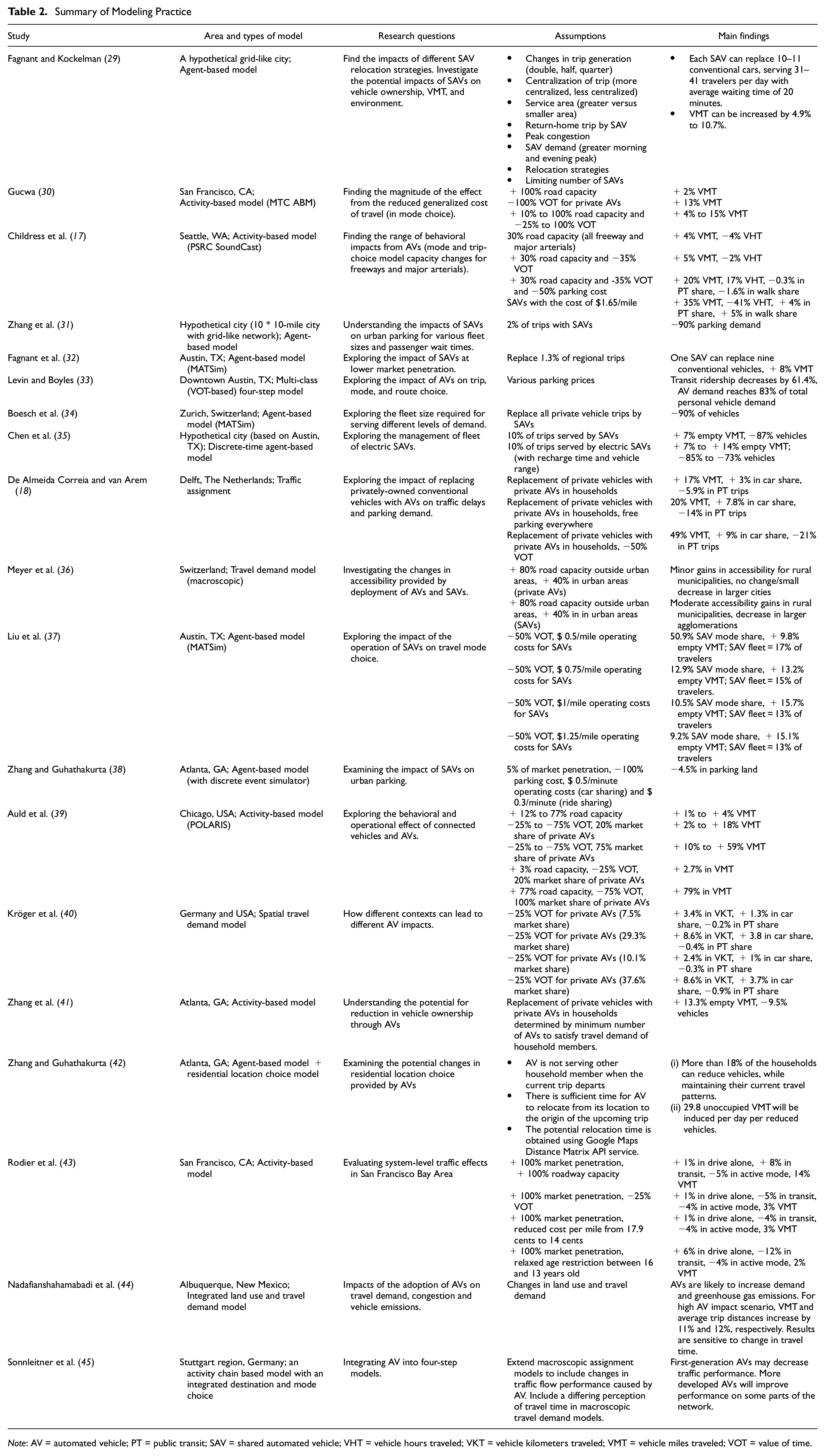
Note: AV = automated vehicle; PT = public transit; SAV = shared automated vehicle; VHT = vehicle hours traveled; VKT = vehicle kilometers traveled; VMT = vehicle miles traveled; VOT = value of time.

This research helps support the efforts to identify the range of potential impacts (in direction and magnitude) of the introduction and rapid adoption of CAVs on travel, VMT, GHG, and criteria pollutant emissions. The study contributes to the transportation research activities in the field in two ways: (a) on the methodological aspect, it builds on literature on the modifications that would be needed in a travel demand model to model CAV impacts; and (b) on the empirical side, it provides support on the evaluation of the impacts of CAV deployment on travel demand and environmental impacts, and the identification of policies to mitigate these impacts.

The remainder of the paper is organized as follows. We first present the modeling framework and scenario design by modifying the California Statewide Travel Demand Model (CSTDM) and integrating it with the EMission FACtor model (EMFAC) and Vision models to compute the related GHG and criteria pollutant emissions. Then the model results for trips, VMT, and emissions are presented for the whole State of California. We also discuss the limitations associated with the modeling structure and assumptions and suggest opportunities for future research.

Methods

In this section, we present the methodology to forecast the potential impacts of CAV deployment using the CSTDM framework for the State of California. As the literature presented in the previous section discusses, CAVs are expected to bring many changes to current transportation systems. Accordingly, we design a list of future travel demand scenarios considering factors and parameters rooted in the literature.

CSTDM Model Framework

The California Statewide Travel Demand Model Version 3.0 (CSTDM V3.0) is an activity-based travel demand model that forecasts all personal travel made by every California resident and all commercial vehicle travel for a typical weekday in fall/spring in a certain scenario projection year. In the CSTDM framework, there are four major model components: (i) short-distance passenger travel model (SDPTM) for passenger trips less or equal to 100 miles; (ii) long-distance passenger travel model (LDPTM) for passenger trips longer than 100 miles, (iii) California state freight forecasting model (CSFFM) for freight trips, and (iv) external travel model (ETM) for trips going into and out of the State of California, shown in Figure 1. The CSTDM V3.0 model uses input from the zone system, networks, population, employment, and zonal properties. Then the major model components—SDPTM, LDPTM, CSFFM, and ETM—compute lists of trip tables by mode at the zonal level, which are then processed by the assignment and skims modules. The outputs of the CSTDM V3.0 include a trip table, loaded network, travel cost, and several summary statistics. The SDPTM and LDPTM are calibrated to match the observed travel patterns from 2010–2012 California Household Travel Survey (2012 CHTS). The forecasting years conducted by Caltrans (California Department of Transportation) range from 2015 toward 2050.

Figure 1.

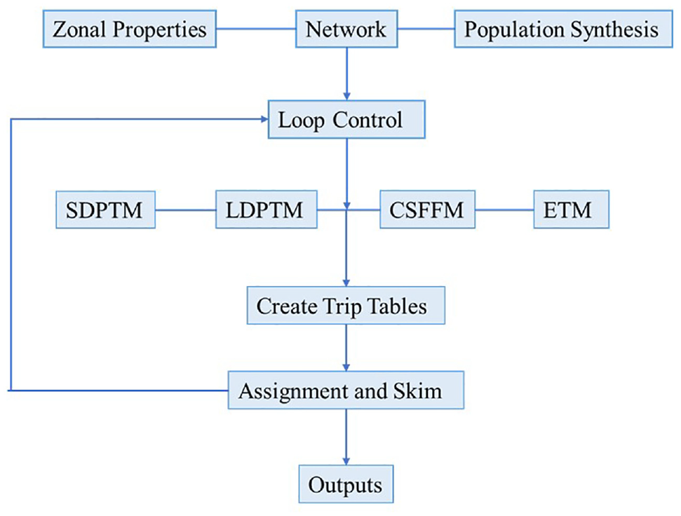
The California Statewide Travel Demand Model Version 3.0 (CSTDM V3.0) modeling framework.

In the CSTDM framework, the entire State of California is divided into 5,454 transportation analysis zones (TAZs) for internal travel and an additional 53 external zones to represent entry/exit points on the state boundary. The model considers four time periods: (i) morning peak from 6:00 to 10:00 a.m.; (ii) midday, from 10:00 a.m. to 3:00 p.m.; 3) evening peak from 3:00 to 7:00 p.m.; and 4) off-peak from 7 p.m. to midnight and from midnight to 6:00 a.m. of the following day.

The SDPTM component considers eight travel modes: 1. SOV (single occupancy auto); 2. HOV2 (high occupancy auto with two persons in the vehicle); 3. HOV3+ (high occupancy auto with three or more persons in the vehicle); 4. Walk to access local transit; 5. Drive to access local transit; 6. Walk; 7. Bicycle; and 8. School bus. The LDPTM component considers five travel modes: 1. SOV; 2. HOV2; 3. HOV 3+; 4. Rail (conventional rail and optional high-speed rail); and 5. Air.

In the demand model framework, SDPTM is designed to follow the procedure as:

Long-term decision (acquire and hold driver’s license, household car ownership, choice of work/school location)

Day patterns (including number, purpose, and time of tours, and stops on tours conditioned by household requirement)

Primary destination choice

Tour mode choice (logit models)

Secondary destination (the destination of all secondary stops on tour)

Trip mode (logit models).

LDPTM is designed to follow the procedure as:

Travel choice model (multinomial logit model)

Party formation model (including base party size, primary traveler model, solo traveler model, and group size model)

Tour property model (including tour duration model, travel day status model, and time of travel model)

Destination choice model (five logit models for different purposes)

Mode choice model, including main mode choice models and access/egress mode choice models (based on California High-Speed Rail Authority high-speed rail model).

CAV Modeling Factors

CAVs are very likely to affect people’s long-term decisions (such as vehicle ownership, residential locations, etc.) and short-term decisions (such as destination choice, mode choice, etc.). In this section, we present the expected impacts of privately-owned and shared CAVs, and our considerations for model components.

Driver’s License

CAVs are expected to provide better mobility and reduce travel inconveniences for the general population, which would bring changes in their long-term decision-making. The population segment not well served by human-driven vehicles should have more opportunities to travel, especially for the young, elderly, and those with physical limitations. It is difficult to modify directly the household vehicle ownership module of the CSTDM, since determining the cost of buying an AV is still a challenge for both the industry and public sectors. Thus, we choose to change the driver’s license module, which is an immediate upstream to vehicle ownership. An individual must obtain a driver’s license to be qualified to own a vehicle. Since there is not a readily available choice model dedicated to CAV because of lack of market penetration, we do not alter the parameters estimated for the driver’s license and vehicle ownership components from the baseline. In this study, we focus on improving the accessibility of vehicles to younger people explicitly by relaxing the age limitation of obtaining a driver’s license to 12 years old or above, the minimum age of prosecution for criminal activities in California. Instead of using a binary logit model to determine whether an individual has a driver’s license, we allow anyone of 12 years or older to have a driver’s license. This would lead to more driver’s licenses and higher vehicle ownership in general. Besides, the senior population has already been classified as capable of owning a vehicle, so we do not explicitly change this module for those population segments. However, by relaxing the VOT and operating cost described in the next sections, various population segments would benefit from implicit improvement in accessibility because of lower travel costs. Combined with other factors, we expect CAVs would enable more accessibility to vehicles for teenagers, the senior population, and people with physical constraints that make it difficult to drive a human-driven vehicle. It is worth noting that legal challenges for operating CAVs still remain, such as liability for human–machine interactions, age restrictions, and physical capabilities of humans and machines ( 46 , 47 ). The treatment in this study is intended to serve only as an initial attempt to quantify the impacts of CAV availability on different user groups. More in-depth research is needed to better understand the legal and ethical aspects of CAVs.

Value of Time

The availability of CAVs would bring more convenience for traveling and enable various in-vehicle activities (such as working, sleeping, and consuming entertainment), thus causing changes to VOT. The convenience of in-vehicle activities within CAVs would lower people’s hesitancy to travel by car. Also, CAVs would then probably make people more tolerant of longer in-vehicle travel time. The original coefficients of VOT in the CSTDM are estimated for human-driven vehicles, which is not suitable for AVs. Thus, we modified the value of travel time to model the change in generalizing cost for mode choice and destination choice. The change in the utility function can be passed down to long-term decisions in the next model since the travel cost and disutility would differ because of a modified cost structure.

Parking Cost

In the CSTDM, parking cost is one feature included in each TAZ in California. Parking cost consists of base cost, time-based cost, and additional cost. Base parking cost represents 1/20 of parking purchased monthly, where this parameter is used in the SDPTM for work and school purposes, since parking is typically purchased on a long-term basis. A regression model is developed in the CSTDM to calculate daily, and hourly costs based on the base price, which is used in the SDPTM and LDPTM for other tour purposes. The additional cost is used to represent the paid parking for visitors.

Parking cost would be very different with the availability of CAVs, in both cost structure and magnitude. For example, a CAV can drive around on its own after dropping off passengers and then return to pick up the passengers in the same or a different location. This behavior would lead to no parking demand being generated at the destination. Travelers can let the vehicle self-park at a farther location with a potentially lower parking cost. Apart from parking choice, land use and curbside management would also be different in the CAV era. Local policymakers would likely consider the disruption caused by frequent pick-ups/drop-offs and make regulations and policy changes accordingly.

Vehicle Operating Cost

Operating costs of CAVs would be different from today’s conventional vehicles because of automated driving technologies, electrification, and other cost components. In the CSTDM, the operating cost ($/mile) consists of fuel and non-fuel operating components. The fuel component cost is largely based on motor gasoline prices and fuel economy (mpg) forecast by the U.S. Energy Information Administration. The non-fuel component is adapted from the California High-Speed Rail Ridership and Revenue model, and it is assumed to be 67% of the fuel component operating cost. The non-fuel component is kept as a fixed constant ($ 0.09/mile) throughout the projected years, based on the assumption that non-fuel operating costs are less volatile than fuel prices.

To account for the impacts of CAVs, we change the projected operating cost provided by Caltrans. This consideration includes assumptions of changes in electrification, vehicle types, and road users. Electrification would likely decrease the operating cost since an increasing number of vehicles (including CAVs) would be electrified, and thus fuel cost components would be directly reduced. Also, operating cost is a good surrogate for congestion pricing and road user charges, meaning extra costs might be imposed when traveling. Thus, in this project, we implement pricing strategies by adjusting the operating cost component in the CSTDM.

It is worth noting that pricing strategy design is important for network operations, especially with the presence of CAVs. However, its impact on large-scale CAV-enabled transportation systems remains unclear ( 48 – 51 ). More advanced tools and further research are needed to incorporate heterogenous microscopic pricing strategies into large-scale statewide travel demand models. Thus, in this work, we assume a homogeneous pricing strategy to keep the statewide modeling tractable.

Highway Network

One of the most direct impacts of automation and vehicle technology is the changes in traffic flow, affecting throughput, stability, safety, and so on. However, these advances cannot be directly implemented under the activity-based framework since the travel decision-making process is not directly affected by vehicle technologies, where the impact can be passed through the change of generalized cost and traffic network operations. With the automation and connectivity features, traffic flow on the highway would be more stable and yield higher throughput. If incidents and congestion are reduced, vehicle travel can be faster, safer, and more reliable. This all leads to the increased level of service of transportation networks. We choose to model changes in vehicle technology and traffic supply by modifying the capacity of the highway network.

Different changes are implemented based on the corresponding facility type, to reflect the different level of improvement or impudence for different driving environments. There are seven facility types in the CSTDM for highway networks: freeway, expressway, major arterial, minor arterial, collector, ramp, and centroid connector (dummy link). We assume the capacity would decrease on ramps because of frequent vehicle-to-vehicle interaction; and capacity is assumed to increase everywhere else except on dummy links.

GHG and Criteria Pollutants Emissions

The GHG and criteria pollutants emissions are calculated based on EMFAC and Vision emission factors. The emission factors depend on regions, fuel types, and vehicle categories. We target four criteria pollutants in this study: carbon dioxide (CO₂), nitrogen oxides (NOx), particulate matter 2.5 (PM2.5), and reactive organic gases (ROG). The processing method is summarized in Figure 2. Emission factors from the Vision model are used for passenger vehicles. The Vision scenario model is a scenario planning tool that incorporates EMFAC 2017 emission rates and scenario-specific forecasted vehicle activities to assess the emission and energy impact of future technologies and policies. The emission factors used in the non-ZEV scenarios and in the ZEV scenario in this study are consistent with the Vision inventories supporting California Air Resources Board (CARB) 2020 Mobile Source Strategy (MSS), respectively, for the business-as-usual (BAU) scenario and the MSS main scenario. The MSS main scenario reflects achieving 100% new sales of passenger vehicles being ZEV or plug-in-hybrid-electric vehicle (PHEV) by 2035. In the MSS Baseline case, VMT by electric vehicles contributes 11% to the total VMT in 2050; in the MSS main case, it contributes 91%. EMFAC emission factors for trucks are retrieved from the EMFAC Web Database (v1.0.2), where we derive the weighted average of emission factors, that is, weighted by VMT for three different truck categories.

Figure 2.

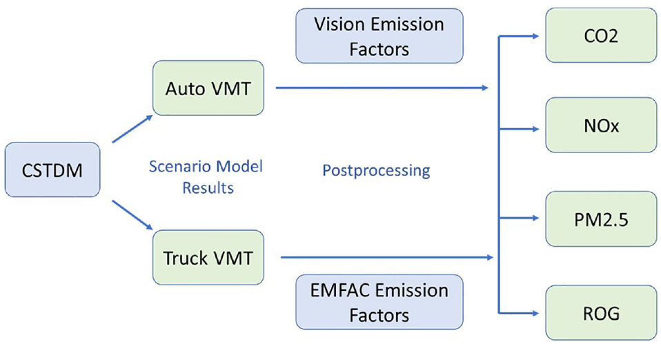
Emission processing method.

Road transportation emissions are calculated separately for passenger vehicles and freight trucks. This could help to segregate the impacts for passenger and freight travel, since the main target is on the passenger side for this project. We follow the procedure below to calculate the emissions for passenger vehicles (auto):

The Vision emission factors originally at GAI (EMFAC’s emission Sub-Area) level are aggregated into county level by taking the countywide averages. (Note that there are 69 GAI areas and 58 counties in the State of California.)

The county-level VMT results are retrieved from the scenario results from the CSTDM.

Statewide emissions are calculated as the sum of the products of county-level VMT and emission factors for CO₂, NOx, PM2.5 and ROG.

The EMFAC model (developed in 2017) is used for truck emission calculations. The emission factors from EMFAC are separated for different vehicle categories, while the results from the CSTDM have only one truck type. Therefore, we derive the weighted average of emission factors, weighted by VMT for three different vehicle categories: light-, medium-, and heavy-duty trucks. The EMFAC 2011 vehicle categories are used to match the categories for the emission factor calculation. We use the weighted average of the “one” truck vehicle type to represent truck emissions for all of California. As a result, we obtain the statewide average of the emission factors for CO₂, NOx, PM2.5, and ROG. Similarly, the VMT at the county level is used as input to calculate pollutants based on corresponding county-level emission factors from Vision and EMFAC in 2050. These results are aggregated at the statewide level.

It is worth mentioning some factors that are held constant for this study. For example, the vehicle ownership choice model remains unchanged simply because there is only one vehicle type for automobiles within the CSTDM, and we cannot differentiate human-driven vehicles and CAVs under this setup. Similarly, we do not implicitly add a shared-use SAV component, which is instead treated as a post-processing step. Because vehicle sharing and ride sharing often require a central controller and agent-based simulation, the sharing mechanism cannot be handled within CSTDM. Other examples include residential location and land use, carried out in the population synthesizer and zonal property inputs in the model. These factors largely rely on urban planning strategy and policy shift for CAVs for the future. Currently, evidence in the literature and practices in the real world can hardly serve as strong evidence for us to project future land use impacts of CAVs. Also, factors in the freight and truck sector are considered outside the scope of this research.

Scenario Design

In this section, we provide the details on how we simulate each scenario in the CSTDM V3.0. All scenarios are modeled for the year 2050 and compared with the baseline Scenario 0 in the discussion of the results and implications for the future of society. We design lower bound (LB, a series) and upper bound (UB, b series) cases for each scenario to provide the ranges of impacts of potential changes, shown in Table 3. Any results within the range are likely to happen for the forecasted year.

Table 3.

Scenario Overview

No.	Scenario	Factor input (compared with Scenario 0)	Off-model processing
0	Baseline (BAU) 2050	*	*
1a	Private CAV (LB)	1. Operating cost −25% 2. Capacity +50% (−20%) 3. Parking cost −25% 4. Driver’s license relaxation 5. Auto VOT −50%	*
1b	Private CAV (UB)	1. Operating cost −25% 2. Capacity +50% (−20%) 3. Parking cost −25% 4. Driver’s license relaxation 5. Auto VOT −50%	1. TAZ level OD trips +15% induced demand for all modes for SD and LD 2. SD deadheading trips +20% SOV, +15% HOV2, +15% HOV3+
2a	Private CAV + Pricing (LB)	1. Operating cost +50% 2. Capacity +50% (−20%) 3. Parking cost −25% 4. Driver’s license relaxation 5. Auto VOT −50%	*
2b	Private CAV + Pricing (UB)	1. Operating cost +50% 2. Capacity +50% (−20%) 3. Parking cost −25% 4. Driver’s license relaxation 5. Auto VOT −50%	1. TAZ level OD trips +15% induced demand for all modes for SD and LD 2. SD deadheading trips +20% SOV, +15% HOV2, +15% HOV3+
3a	Private CAV + ZEV (LB)	1. Operating cost −25% 2. Capacity +50% (−20%) 3. Parking cost −25% 4. Driver’s license relaxation 5. Auto VOT −50%	Post-processing on ZEV emission
3b	Private CAV + ZEV (UB)	1. Operating cost −25% 2. Capacity +50% (−20%) 3. Parking cost −25% 4. Driver’s license relaxation 5. Auto VOT −50%	1. TAZ level OD trips +15% induced demand for all modes for SD and LD 2. SD deadheading trips +20% SOV, +15% HOV2, +15% HOV3+ 3. Post-processing on ZEV emission
4a	Shared CAV (LB)	1. Operating cost −25% 2. Capacity +50% (−20%) 3. Parking cost −25% 4. Driver’s license relaxation 5. Auto VOT −50%	1. For SD TAZ level OD, move 10% of SOV trips to HOV2 (get 60%), and HOV3+(get 40%); move 40% of PT trips to HOV2 (get 70%) and HOV3+ (get 30%) 2. SD deadheading +10% HOV2, +10% HOV3+
4b	Shared CAV (UB)	1. Operating cost −25% 2. Capacity +50% (−20%) 3. Parking cost −25% 4. Driver’s licenses relax to age 12 5. Auto VOT −50%	1. TAZ level OD trips +15% induced demand for all modes for SD and LD 2. For SD TAZ level OD, move 10% of SOV trips to HOV2 (get 60%), and HOV3+ (get 40%); move 40% of PT trips to HOV2 (get 70%) and HOV3+ (get 30%) 3. SD deadheading +20% SOV, +20% HOV2, +20% HOV3
5a	Shared CAV + pricing (LB)	1. Operating cost +50% 2. Capacity +50% (−20%) 3. Parking cost −25% 4. Driver’s licenses relax to age 12 5. Auto VOT −50%	1. For SD TAZ level OD, move 10% of SOV trips to HOV2 (get 60%), and HOV3+ (get 40%); move 40% of PT trips to HOV2 (get 70%) and HOV3+ (get 30%) 2. SD deadheading +10% HOV2, +10% HOV3+
5b	Shared CAV + pricing (UB)	1. Operating cost +50% 2. Capacity +50% (−20%) 3. Parking cost −25% 4. Driver’s licenses relax to age 12 5. Auto VOT −50%.	1. TAZ level OD trips +15% induced demand for all modes for SD and LD 2. For SD TAZ level OD, move 10% of SOV trips to HOV2(get 60%), and HOV3+(get 40%); move 40% of PT trips to HOV2 (get 70%), HOV3+ (get 30%) 3. SD deadheading +20% SOV, +20% HOV2, +20% HOV3
6a	Shared CAV + ZEV (LB)	1. Operating cost −25% 2. Capacity +50% (−20%) 3. Parking cost −25% 4. Driver's license relaxation 5. Auto VOT −50%	1. For SD TAZ level OD, move 10% of SOV trips to HOV2 (get 60%), and HOV3+ (get 40%); move 40% of PT trips to HOV2 (get 70%) and HOV3+ (get 30%) 2. SD deadheading +10% HOV2, +10% HOV3+ 3. Post-processing on ZEV emissions
6b	Shared CAV + ZEV (UB)	1. Operating cost −25% 2. Capacity +50% (−20%) 3. Parking cost −25% 4. Driver's license relaxation 5. Auto VOT −50%	1. TAZ level OD trips +15% induced demand for all modes for SD and LD 2. For SD TAZ level OD, move 10% of SOV trips to HOV2 (get 60%), and HOV3+ (get 40%); move 40% of PT trips to HOV2 (get 70%), HOV3+ (get 30%) 3. SD deadheading +20% SOV, +20% HOV2, +20% HOV3 4. Post-processing on ZEV emissions

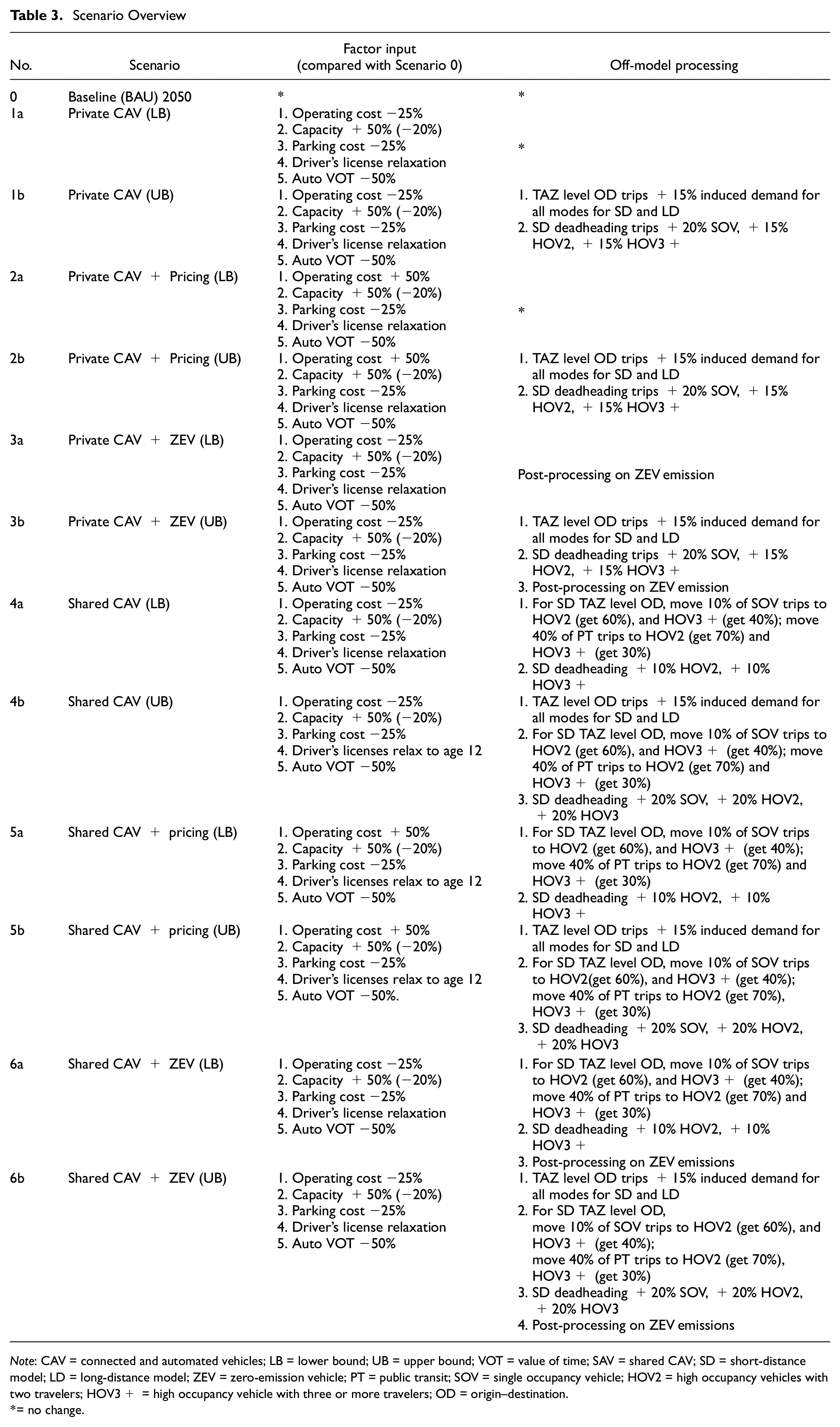
Note: CAV = connected and automated vehicles; LB = lower bound; UB = upper bound; VOT = value of time; SAV = shared CAV; SD = short-distance model; LD = long-distance model; ZEV = zero-emission vehicle; PT = public transit; SOV = single occupancy vehicle; HOV2 = high occupancy vehicles with two travelers; HOV3+ = high occupancy vehicle with three or more travelers; OD = origin–destination.

= no change.

Scenario 0. Baseline (BAU)

This study uses the 2050 Caltrans scenario as a baseline for comparison with the other scenarios. The 2050 baseline scenario takes in the projected zonal properties, networks, and lists of socioeconomic data as input. The daily activity pattern is computed from a predetermined day pattern pool. Average auto occupancy for HOV3+ vehicles is set as 3.6. In the forecasting year 2050, the baseline operating cost is $ 0.20. A high-speed rail option is available in the long-distance travel model. CAVs are not included in the baseline scenario. The outputs include trips by modes by time period at the TAZ level. VMT and VHT (vehicle miles traveled) are also generated for separate modes. The following scenarios are built on top of the baseline scenario.

Scenario 1. Private CAV

This scenario assumes the highest penetration of personally owned AVs in the year 2050 (Scenario 1a Private CAV LB). CAVs are assumed to be only available as private options with a 100% penetration rate based on the literature specified in Table 2. The range of CAV penetration rate is dependent on various beliefs about how CAV technology would be developed in the future. Such high penetration rates would ensure that most of the benefits from the CAV deployment are available to travelers. The VOT of using the private car mode is assumed to decrease by 50%. This is generally because of the convenience of traveling with a privately-owned CAV, as the “driver” could conduct other activities in a CAV. Here we assume the VOT is decreased for single occupancy vehicles (SOVs), high occupancy vehicles with two travelers (HOV2s), and high occupancy vehicles with three or more travelers (HOV3+). Note that the VOT is kept unchanged for transit users.

The overall vehicle operating cost per mile in 2010 currency value is set at $0.15, the same for all passenger vehicles. The network capacity is treated separately for different facility types of the highway network. The capacity is assumed to increase by 50% for the majority of the highway, including freeways, expressways, major/minor arterials, and collectors. The capacity of the ramp section is assumed to decrease by 20%, because of more friction induced by merging and splitting of CAV vehicles. The parking cost, based on the zonal properties corresponding to each TAZ, is assumed to decrease by 25%. This treatment is based on two assumptions: (i) a lower parking cost would lead to a higher probability of parking, to mimic the possibilities that CAVs could park on their own and maybe at a different place (usually farther from the central business district) with a lower cost; (ii) a lower parking cost would induce a low total travel cost, thus causing more potential travels. The availability of a driver’s license, originally developed as a binary logit model for each individual, is now relaxed into a simpler if condition. Note that having a driver’s license is the precondition of owning a vehicle, so we anticipate seeing higher vehicle ownership within the model results because of this adjustment.

Next, based on the model outputs, we study the range of demand expansion and deadheading for the upper bound case (Scenario 1b Private CAV UB). We create an upper bound case to account for the extra VMT for empty miles and mode share penalty based on the setup for Scenario 1a. Trip generation will likely differ in the CAV era, especially since CAVs will be a brand-new advanced transportation mode. With much lower travel costs for CAVs compared with human-driven vehicles on current infrastructure, more trip generation is anticipated systemwide. However, the trip generation process in the CSTDM mainly depends on sociodemographic and home/work locations, which is constant in the CSTDM setup. This is not realistic with the expectations from the literature on a CAV future, which might lead to substantial induced demand. Thus, we apply a 15% increase in demand for all travel modes (including auto modes, transit, rail, and air) to account for the induced demand. This can be considered as even a conservative estimate when compared with the findings from recent studies ( 52 ). Further, the availability of CAVs would also generate extra deadheading that is not captured in the original CSTDM framework. Thus, we assume that the impacts of deadheading would translate in increasing SOV trips by 20%, HOV2 trips by 15%, and HOV3+ trips by 15%. Therefore, we model Scenario 1b (upper bound), including two main additional assumptions:

TAZ level OD trips (induced demand; OD = origin–destination): increase 15% for all modes in short-distance model (SD) and long-distance model (LD);

SD deadheading trips: SOV increase 20%, HOV2 increase 15%, HOV3+ increase 15%.

These two adjustments are used as a proxy for the induced demand and extra travel generated for ZEV pick-up and return trips.

Scenario 2. Private CAV + Pricing

In this scenario, we model a policy with road user charges, based on the private CAV scenario (Scenario 1). We assume that only privately-owned CAVs are available, with a penetration rate of 100%. Adding road user charges would directly increase travel costs for travelers by automobile. There have been discussions on road user charge and congestion pricing in the literature. For example, configurations and design principles of static and dynamic pricing schemes are thoroughly discussed by Tsekeris and Voß. ( 53 ). Another survey paper summarizes the congestion pricing types as: facility-based, cordon, zonal, distance-based, and degree of time-based schemes ( 54 ). The pricing strategy should reflect considerations of the dynamic traffic flow pattern in the networks, variable travel demand, travelers’ preference, vehicle fleet composition, equity, and mobility market externalities. However, it is still unclear how to determine the geographical boundary of such change at the state level. A localized policy would potentially bring better overall effectiveness yet giving implementation challenges at the large scale. On the other hand, a statewide policy is easier to quantify in the travel demand model framework, however, it ignores the needs across communities with various mobility needs and infrastructure support.

In this study we assume the same changes are applied to all trips made by passenger vehicles so that the overall vehicle operating cost can reflect the systemwide adjustment. The operating cost parameter is assumed to increase by 50% over the BAU cost and set as $ 0.30/mile. Since the operating cost component is not directly dependent on the highway network, it is safe to assume that network capacity changes by the same amount as in the private CAV scenario. Similarly, VOT, parking cost, and driver’s license are kept the same as in the private CAV scenario. Similar to Scenario 1b, we make demand expansion and deadheading adjustments for the upper bound case.

Scenario 3. Private CAV + ZEV

Because of the limitation that only one passenger vehicle type is available in the CSTDM, we choose to use post-processing on emission factors to estimate the potential impacts of electrified CAVs. This treatment would ignore the potential changes in travel patterns and travel impedance caused by electrification, but it still provides some insights into how emissions would be affected in a scenario with wide ZEV adoption. We assume total 91% VMT are zero-emission, based on Vision MSS main scenario assumption. This scenario is computed by post-processing using various emission factors from the Vision and EMFAC emission model in combinations with the model assumptions and results for Scenario 1a and 1b.

Scenario 4. Shared CAV

The CSTDM V3.0 cannot properly incorporate the shared use of CAVs (i.e., SAVs), especially for complicated vehicular behavior for pick-up and repositioning. We assume the SAV fleet will provide a TNC-like mobility service in this scenario. Everyone could request SAV trips given the availability of the service. We divide the potential impacts of SAVs into three categories: (i) Trip generation: more trips because of lower travel costs and the convenience of SAVs; (ii) Mode share: a portion of single occupancy vehicle trips would shift to shared trips and some of the public transit trips would also shift to auto trips; and (iii) Deadheading and repositioning: extra VMT for zero-occupancy vehicle travel.

Additional induced demand would be generated with the availability of SAVs. One thing to note is that the amount of deadheading is closely related to the demand density and fleet service provided in the region. With more service provided, the VMT caused by deadheading for repositioning would be proportionally smaller. Based on the Clean Miles Standard analysis from CARB, the statewide average deadheading of TNC VMT is 38.5%. In this scenario, we assume the deadheading contributed to 40% of the total VMT for the entire state. If each trip contributes the same amount of VMT on average, we have 40% of trips as repositioning trips. If we assume 50% of the SOV trips would be conducted via SAV mode, provided enough SAV fleet supply, the extra trips for deadheading would be 20% of the total auto trips. Accordingly, our assumption is consistent with CARB’s Clean Miles Standard analysis. Thus, the off-model adjustments are applied for upper bound Scenario 4b.

Scenario 5. Shared CAV + Pricing

For Scenario 5, we want to evaluate the combination of pricing (Scenario 2) and sharing (Scenario 4) strategies. The assumptions are based on the setup used in the corresponding two scenarios.

Scenario 6. Shared CAV + ZEV

For Scenario 6, the electrification scenario for private CAV + ZEV, we use a post-processing approach to account for the reduced GHG and criteria pollutant emissions for shared CAV + ZEV. Based on the CABR’s MSS main scenario in the Vision model described in the “CAV Modeling Factors – GHG and Criteria Pollutants Emission” section, we assume 91% of VMT from Scenario 4 (Sharing) are zero-emission VMTs.

Empirical Results

Trips, VMT, and VHT

We report here the model results for a regular weekday for the entire State of California. More detailed results can be found in the extended report by the authors ( 55 ). As previously discussed, our modeling approach assumes there are no travel behavior differences between the ZEV scenarios and non-ZEV scenarios. Accordingly, the travel-related metrics for the ZEV scenarios (3a, 3b, 6a, and 6b) are not duplicated here as they are identical to those from Scenarios 1a, 1b, 4a, and 4b, respectively. Figures 3 and 4 summarize the range of auto VMT in the various scenarios. The results of auto VMT range from 1,196 million vehicle miles to 1,616 million vehicle miles for Scenarios 1a and 1b, where the induced demand contributes 15% and deadheading contributes 20% of the differences. For 2a and 2b, the results of auto VMT range from 906 million to 1,217 million. Note that the lower bound VMT for this scenario is lower than the baseline 2050 scenario, which shows how, according to the CSTDM outputs, the pricing strategy could be effective in calming total auto VMT. For scenarios 4a and 4b, auto VMT ranges from 1,174 million to 1,652 million. The auto VMT of 5a and 5b range from 904 million to 1,185 million.

Figure 3.

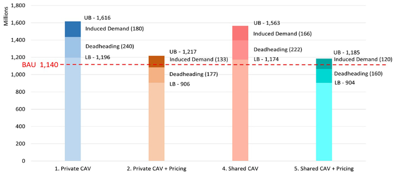
Range of auto vehicle miles traveled (VMT) in the modeling scenarios.

Figure 4.

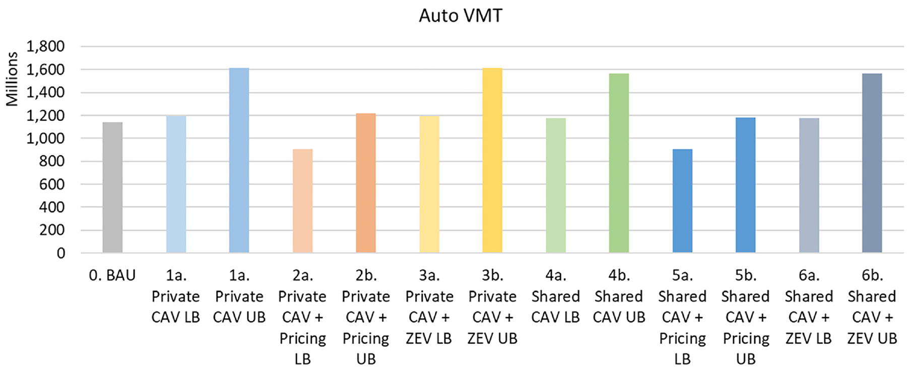
Auto vehicle miles traveled (VMT).

We then show the total number of trips and number of trips by mode, including auto, short-distance transit, conventional rail, high-speed rail, in-state air, walk/bike, and school bus, in Figure 5. Several more detailed breakdown tables are included in Appendix A. For both the private CAV scenario and shared CAV scenario, there are slight increases in the number of passenger vehicle (auto) trips in lower-bound scenarios. There is a decrease in total trips and VMT in Scenario 2a, meaning that, according to the CSTDM forecasts, the increased operating cost would hinder people from traveling, through both reductions in the trip volumes and average trip distances. We also observe a substantial mode shift toward automobiles from transit. The number of rail and in-state air trips is largely reduced with the availability of CAVs. For the private CAV scenario, the number of trips and VMT of autos slightly increases compared with the baseline. However, the VMT of auto decreases in the pricing strategies scenario, because of the penalty of higher vehicle operating costs. Similar effects on VMT are observed in the shared CAV + pricing scenario. This shows the effectiveness of scenarios that involve pricing strategies and policies to promote the deployment of SAVs. In particular, the scenario results show how person trips in such a situation increase without a sizable total VMT, thanks to a reduction in the average trip distances and an increase in vehicle occupancy.

Figure 5.

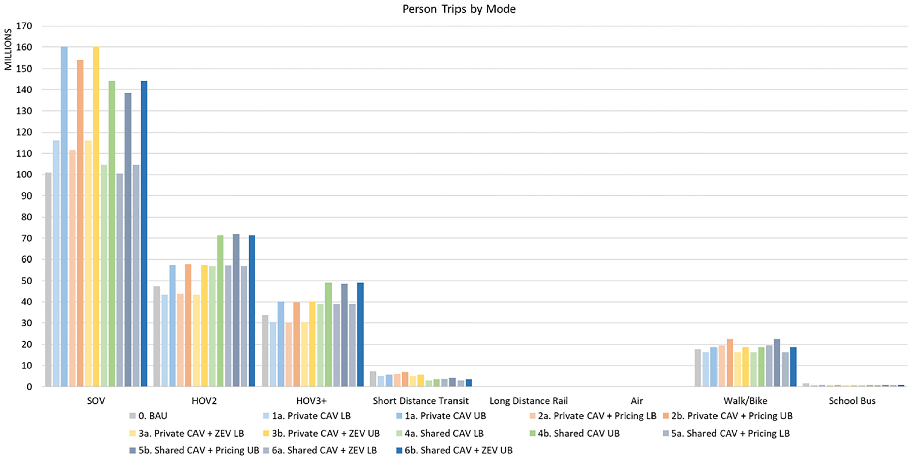
Person trips by mode.

Total trip numbers remain relatively stable across all lower bound scenarios, partially because of the design of the CSTDM. The trip generation step largely depends on household and employment locations and socioeconomic, which are held constant. The adjusted travel cost functions in our scenarios do not have much impact on the upstream trip generation. However, a difference of approximately 50 million person trips separates the lower bound and upper bound cases, highlighting that induced demand and extra deadheading will likely cause future travel in a CAV-dominated era.

Next, we show the spatial pattern differences in absolute value and percentage change of auto VMT compared with the baseline 2050 scenario in Figure 6. In the BAU baseline case for the year 2050, most of the auto VMT are generated in the Sacramento, San Francisco Bay, Greater Los Angeles, and San Diego regions. Relatively low auto VMT are forecast in the remaining lower-population regions. For the private CAV and shared CAV scenarios, the majority of the absolute changes in auto VMT are in areas with already high auto VMT. However, the San Joaquin Valley region reports a rather high relative change. Possibly this is because the networks in high auto VMT areas are already running at capacity, and higher demand for CAV would not greatly affect the already congested network. Instead, the San Joaquin region has greater capacity to allow more CAV trips and higher VMT and is also crossed by long-distance travel to/from other regions in California.

Figure 6.

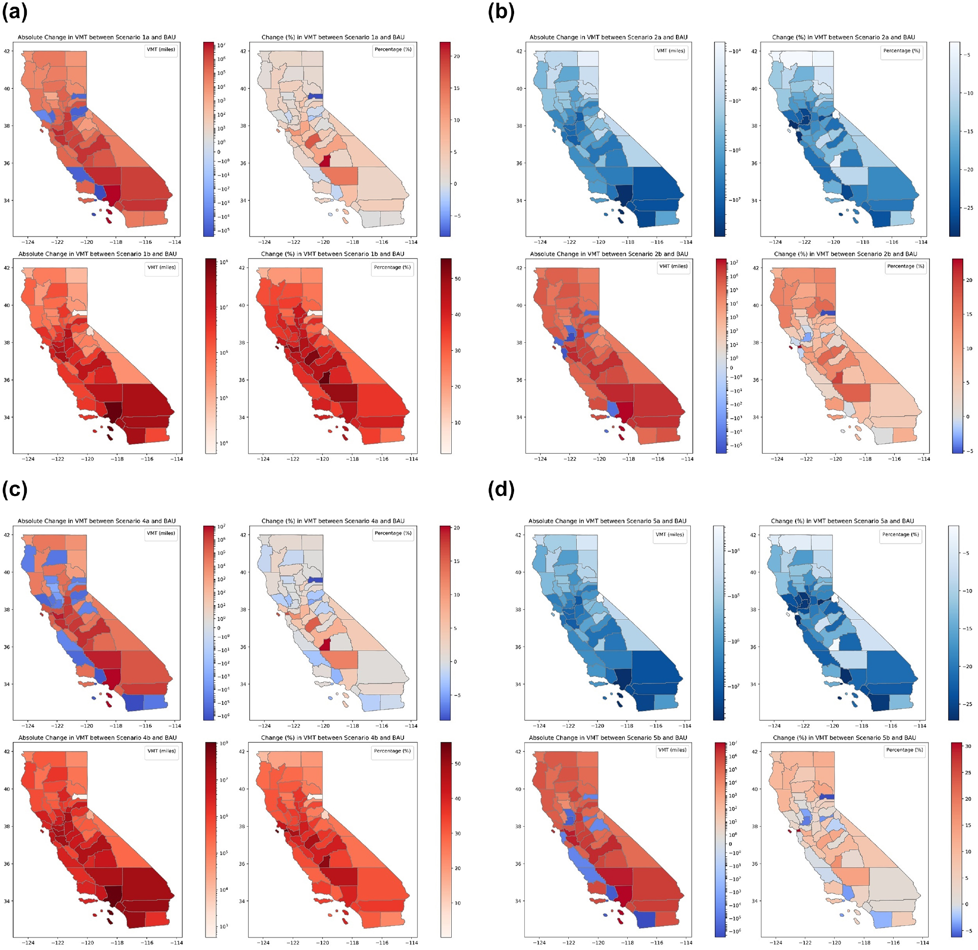
Spatial plots for VMT absolute change and percentage change, respectively: (a) Estimated VMT in Scenarios 1a and 1b, (b) Estimated VMT in Scenarios 2a and 2b, (c) Estimated VMT in Scenarios 4a and 4b, and (d) Estimated VMT in Scenarios 5a and 5b.

GHG and Criteria Pollutant Emissions

Based on the model results, we evaluated the environmental impacts of CAV deployment in California. Total statewide percentage changes for auto emissions and total (auto and truck) emissions are shown in Figure 7. We observe increases in auto pollutants in the private CAV and shared CAV scenarios, while both the private and shared ZEV scenarios yield lower levels of pollutant emissions. With the high penetration rate of ZEVs, we observed a dramatic reduction in auto emissions. The private CAV + pricing and shared CAV + pricing scenarios achieve a substantial containment of total emissions, though the real abatement of GHG and other criteria pollutant emissions is achieved in the ZEV scenarios.

Figure 7.

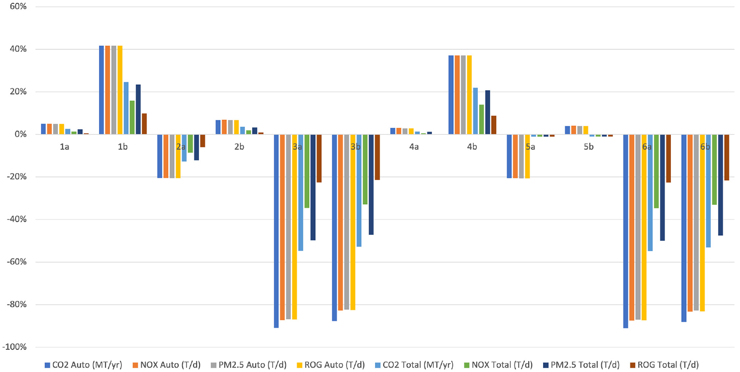
Percentage change of criteria pollutants for the year 2050 compared with baseline.

Discussion

Many metropolitan planning organizations and other transportation agencies have adopted activity-based models to support transportation planning decisions and evaluate infrastructure projects. Activity-based models, such as the CSTDM, overcome the limitations in the classical four-step model by generating a synthetic population of households and individuals and modeling their activity participation and travel choices.

While activity-based models provide many benefits in their increased ability to model realistic individual behaviors and forecast the resulting travel demand impacts, they have several limitations. First, a general limitation in modeling CAV deployment impacts is that while alternatives to owning and driving a private vehicle are becoming increasingly available, whether and how these services and technologies will be accessible to the various segments of the population in different areas remains unknown. Similarly, research to date only provides limited insights into the behavioral changes that these alternative solutions might cause. The second limitation is rooted in the activity-based modeling framework in general. In this study, our assumption is that the statewide activity-based model can capture the impacts of CAVs through the changes in the travel behavior of the population. The fundamental behavioral assumptions rely on how people would perceive CAVs in the future and how they would adjust their corresponding daily travel behavior. While we implement several changes in the modeling framework to account for the behavioral changes prompted by CAV availability, we hold constant some other functions, estimated coefficients, and constants in the model. Third, we use a model that was developed using survey data from past years, while many uncertainties remain about the future. This includes changes in lifestyle, technology, urban form, and policy that might modify the underlying behavioral framework with which individuals make choices in their everyday lives. This is also caused by the introduction of new CAV travel modes, which will bring drastic changes to the transportation system, household organization, and individuals’ activities and choices. Thus, there is no guarantee that the equations estimated using data from the past will hold in the future, given advanced in-vehicle technologies, intelligent transportation systems, and new household vehicle ownership options.

The estimations of the model coefficients usually remain valid for modeling applications to scenarios that fit in a certain range of applicability. When we introduce into the model modified assumptions and a new technology that will likely cause large modifications in individual behaviors, as is the case of CAVs, the assumptions about behaviors (and calibration procedures for the model base year) that form the basis for the model might no longer hold true. The model assumptions and calibration practices usually adopted in the development of activity-based models might actually limit the amount of change in forecast travel demand, constraining the results to a range that is more conventional and closer to the baseline scenario. This type of problem is not unusual in travel demand forecasting models, especially in cases when the model is somewhat over-fitted to replicate the observed traffic volumes in the baseline scenario during the calibration and validation processes.

Further, if CAVs cause reductions in travel costs in a future dominated by vehicle automation, CAV deployment may well lead to modifications in land use that are not accounted for in this study. Another limitation is that the model seems to be designed and calibrated so that travel cost is prioritized. Additional investigation of these topics and evaluation of the model elasticities and overall ability to forecast the potential impacts of the CAV deployment are recommended in future research.

It should be also noted that we are ignoring the disruption to transportation and the whole of society caused by the COVID19 pandemic. Travel behavior choices might be different from the pre-COVID era, with long-term effects on telecommuting, car dependency, and activity patterns that are still difficult to predict at the time of writing this paper.

Despite the many limitations that might affect our results, this study provides important evidence to inform policy frameworks to advance a sustainable CAV deployment in California, as well as in other parts of the USA and abroad. In particular, the study systematically discusses the many impacts that CAVs might have on future society and transportation, including those that could not be empirically assessed in the modeling application. CAVs might lead to many desirable outcomes, including increased safety, reduced traffic fatalities, and increased mobility for those with unmet mobility needs, and they will considerably increase quality of life, especially for individuals with disabilities and mobility impairments. But they might also cause a sharp increase in the use of automobiles, together with the risk of increased car dependence in society, decreased demand for public transit, and reductions in active travel.

Conclusion

This paper explored the potential impacts of the deployment of CAVs by modifying an activity-based travel demand model based on various travel assumptions and policies, such as high market penetration of electric-powered transportation and the introduction of road pricing. In detail, we investigated the factors influencing the adoption and willingness to pay for CAVs, as well as the likely impacts that CAV deployment will have on future travel. CAV availability will remarkably influence society, modifying the way people live, travel, shop, socialize, and participate in various activities.

Our results show how public transit, active modes, long-distance rail, and in-state air travel could experience a significant reduction in both their mode share and total number of trips in a future dominated by CAVs unless sufficient policies are implemented. The total number of trips would be less affected than VMT and VHT, which are found to be rather sensitive to auto travel costs. This difference in sensitivity might be partially an artifact of the specific modeling assumptions and structure of the CSTDM framework and not entirely a realistic feature of future transportation, and more research is recommended to investigate the topic. Also, the scenarios were developed before the COVID-19 pandemic, and the model coefficients were calibrated and validated based on a regular year before the interruption of COVID-19. Thus, the results of the application of CSTDM in this project do not take into consideration the short- or long-term impacts of the pandemic.

Even considering these limitations, the results highlight how the eventual implementation of pricing strategies and congestion pricing policies could have a significant impact on mitigating increases in travel demand caused by CAV deployment. The study also shed light on the benefit of mitigating emissions that ZEV policies would bring into transportation systems. The results from this study can help inform policymakers and metropolitan planning organizations on the likely impacts that CAV deployment could have on transportation and on GHG and other pollutant emissions.

More broadly, several potential strategies could be deployed to mitigate the eventual negative externalities associated with CAV deployment. These include:

Establish programs that result in the deployment of driverless vehicles as shared rather than privately-owned vehicles, such that they will be subject to the Clean Miles Standard and considerably reduce emissions by 2030;

Adopt a timeline of rapid vehicle electrification for privately-owned CAVs.

Develop a clear incentive system for pricing the climate impacts of travel—consider charging drivers using a GHG/passenger-mile basis;

Create programs that deploy CAVs to address first- and last-mile gaps, connecting more riders to line haul transit;

Ensure CAV fleets include a range of vehicle types so that demand can be right-sized and consume less energy;

Encourage local planning jurisdictions to work to integrate CAVs into complete streets planning, so that CAVs improve livability, safety, and comfort on surface streets;

Ensure local planning efforts are rooted in direct community engagement so that community members can inform planners on how the introduction of CAVs could improve the accessibility and affordability of goods and services, particularly among historically underserved populations.

Supplemental Material

sj-docx-1-trr-10.1177_03611981231186984 – Supplemental material for Impacts of Connected and Automated Vehicles on Travel Demand and Emissions in California

Supplemental material, sj-docx-1-trr-10.1177_03611981231186984 for Impacts of Connected and Automated Vehicles on Travel Demand and Emissions in California by Ran Sun, Giovanni Circella, Miguel Jaller, Xiaodong Qian and Farzad Alemi in Transportation Research Record

Footnotes

Acknowledgements

The authors Farzad Alemi and Xiaodong Qian undertook this study while working at the University of California, Davis. Xiaodong Qian is now with Department of Civil and Environmental Engineering at Wayne State University and Farzad Alemi is now with Google. This study also capitalizes on the work developed in several previous research projects carried out at the Institute of Transportation Studies at UC Davis and the contributions from a workshop with several qualified modeling experts held at UC Davis.

Author Contributions

The authors confirm contribution to the paper as follows: study conception and design: G. Circella, R. Sun, M. Jaller, F. Alemi; data collection: R. Sun; analysis and interpretation of results: R. Sun, G. Circella, X. Qian; draft manuscript preparation: R. Sun, G. Circella, M. Jaller, X. Qian. All authors reviewed the results and approved the final version of the manuscript.

Declaration of Conflicting Interests

The author(s) declared no potential conflicts of interest with respect to the research, authorship, and/or publication of this article.

Funding

The author(s) disclosed receipt of the following financial support for the research, authorship, and/or publication of this article: This work was prepared as part of a project funded by the California Air Resources Board. Additional funding was provided by the 3 Revolutions Future Mobility Program of UC Davis.

ORCID iDs

Ran Sun

Giovanni Circella

Miguel Jaller

Xiaodong Qian

Farzad Alemi

Supplemental Material

Supplemental material for this paper is available online.

The opinions expressed in this paper are those of the authors and not necessarily those of the California Air Resources Board. This paper does not constitute a standard, specification, or regulation.

References

VanderWerf

Shladover

Miller

M. A.

Conceptual Development and Performance Assessment for the Deployment Staging of Advanced Vehicle Control and Safety Systems. PATH Research Report UCB-ITS-PRR-2004-22. Institute of Transportation Studies, University of California, Berkeley, CA, 2004.

Bierstedt

Gooze

Gray

Peterman

Raykin

Walters

Effects of Next-Generation Vehicles on Travel Demand and Highway Capacity. FP Think Working Group, 2014.

Gong

Cooperative Platoon Control for a Mixed Traffic Flow Including Human Drive Vehicles and Connected and Autonomous Vehicles. Transportation Research Part B: Methodological, Vol. 116, 2018, pp. 25–61.

Liu

Nie (Marco)

Managing Partially Automated Network Traffic Flow: Efficiency vs. Stability. Transportation Research Part B: Methodological, Vol. 114, 2018, pp. 300–324.

Hatipoglu

Özguner

Ü.

Redmill

K. A.

Automated Lane Change Controller Design. IEEE Transactions on Intelligent Transportation Systems, Vol. 4, No. 1, 2003, pp. 13–22.

Wischhof

Ebner

Rohling

Information Dissemination in Self-Organizing Intervehicle Networks. IEEE Transactions on Intelligent Transportation Systems, Vol. 6, No. 1, 2005, pp. 90–101.

Shladover

S. E.

X. Y.

Impacts of Cooperative Adaptive Cruise Control on Freeway Traffic Flow. Transportation Research Record: Journal of the Transportation Research Board, 2012. 2324: 63–70.

Talebpour

Mahmassani

H. S.

Influence of Connected and Autonomous Vehicles on Traffic Flow Stability and Throughput. Transportation Research Part C: Emerging Technologies, Vol. 71, 2016, pp. 143–163.

Olia

Razavi

Abdulhai

Abdelgawad

Traffic Capacity Implications of Automated Vehicles Mixed With Regular Vehicles. Journal of Intelligent Transportation Systems, Vol. 22, No. 3, 2018, pp. 244–262.

10.

Adebisi

Guo

Schroeder

Cesme

Bibeka

Morgan

Highway Capacity Manual Capacity Adjustment Factor Development for Connected and Automated Traffic at Signalized Intersections. Journal of Transportation Engineering, Part A: Systems, Vol. 148, No. 3, 2021, p. 04021121.

11.

Amini

Omidvar

Elefteriadou

Optimizing Operations at Freeway Weaves With Connected and Automated Vehicles. Transportation Research Part C: Emerging Technologies, Vol. 126, 2021, p. 103072.

12.

Fagnant

D. J.

Kockelman

Preparing a Nation for Autonomous Vehicles: Opportunities, Barriers and Policy Recommendations. Transportation Research Part A: Policy and Practice, Vol. 77, 2015, pp. 167–181.

13.

Stephens

T. S.

Gonder

Chen

Lin

Liu

Gohlke

Estimated Bounds and Important Factors for Fuel Use and Consumer Costs of Connected and Automated Vehicles [Internet]. 2016. NREL. www.nrel.gov/publications.

14.

Abrantes

P. A. L.

Wardman

M. R.

Meta-Analysis of UK Values of Travel Time: An Update. Transportation Research Part A: Policy and Practice, Vol. 45, No. 1, 2011, pp. 1–17.

15.

Yap

M. D.

Correia

van Arem

Preferences of Travellers for Using Automated Vehicles as Last Mile Public Transport of Multimodal Train Trips. Transportation Research Part A: Policy and Practice, Vol. 94, 2016, pp. 1–16.

16.

Malokin

Circella

Mokhtarian

P. L.

How Do Activities Conducted While Commuting Influence Mode Choice? Using Revealed Preference Models to Inform Public Transportation Advantage and Autonomous Vehicle Scenarios. Transportation Research Part A: Policy and Practice, Vol. 124, 2019, pp. 82–114.

17.

Childress

Nichols

Charlton

Coe

Using an Activity-Based Model to Explore the Potential Impacts of Automated Vehicles. Transportation Research Record: Journal of the Transportation Research Board, 2015. 2493: 99–106.

18.

de Almeida Correia

G. H.

van Arem

Solving the User Optimum Privately Owned Automated Vehicles Assignment Problem (UO-POAVAP): A Model to Explore the Impacts of Self-Driving Vehicles on Urban Mobility. Transportation Research Part B: Methodological, Vol. 87, 2016, pp. 64–88.

19.

Gurumurthy

K. M.

Kockelman

K. M.

Modeling Americans’ Autonomous Vehicle Preferences: A Focus on Dynamic Ride-Sharing, Privacy & Long-Distance Mode Choices. Technological Forecasting and Social Change, Vol. 150, 2020, p. 119792.

20.

Bansal

Kockelman

K. M.

Singh

Assessing Public Opinions of and Interest in New Vehicle Technologies: An Austin Perspective. Transportation Research Part C: Emerging Technologies, Vol. 67, 2016, pp. 1–14.

21.

Krueger

Rashidi

T. H.

Rose

J. M.

Preferences for Shared Autonomous Vehicles. Transportation Research Part C: Emerging Technologies, Vol. 69, 2016, pp. 343–355.

22.

Haboucha

C. J.

Ishaq

Shiftan

User Preferences Regarding Autonomous Vehicles. Transportation Research Part C: Emerging Technologies, Vol. 78, 2017, pp. 37–49.

23.

Pourrahmani

Jaller

Maizlish

Rodier

Health Impact Assessment of Connected and Autonomous Vehicles in San Francisco Bay Area. Transportation Research Record: Journal of the Transportation Research Board, 2020. 2674: 898–916.

24.

Chapin

Stevens

Crute

Crandall

Rokyta

Washington

Envisioning Florida’s Future: Transportation and Land Use in an Automated Vehicle World. Florida State University Department of Urban & Regional Planning, Tallahassee, FL, 2016.

25.

Crute

Riggs

Chapin

T. S.

Stevens

Planning for Autonomous Mobility. PAS Report 592. American Planning Association, 2018. https://www.planning.org/publications/report/9157605/

26.

Adnan

Nordin

S. M.

bin Bahruddin

M. A.

Ali

How Trust Can Drive Forward the User Acceptance to the Technology? In-Vehicle Technology for Autonomous Vehicle. Transportation Research Part A: Policy and Practice, Vol. 118, 2018, pp. 819–836.

27.

Conlon

Lin

Greenhouse Gas Emission Impact of Autonomous Vehicle Introduction in an Urban Network. Transportation Research Record: Journal of the Transportation Research Board, 2019. 2673: 142–152.

28.

Jenn

Evaluating the Emission Benefits of Shared Autonomous Electric Vehicle Fleets: A Case Study in California. Applied Energy, Vol. 323, 2022, p. 119638.

29.

Fagnant

D. J.

Kockelman

K. M.

The Travel and Environmental Implications of Shared Autonomous Vehicles, Using Agent-Based Model Scenarios. Transportation Research Part C: Emerging Technologies, Vol. 40, 2014, pp. 1–13.

30.

Gucwa

Mobility and Energy Impacts of Automated Cars. Proc., Automated Vehicles Symposium, San Francisco, 2014.

31.

Zhang

Guhathakurta

Fang

Zhang

Exploring the Impact of Shared Autonomous Vehicles on Urban Parking Demand: An Agent-Based Simulation Approach. Sustainable Cities and Society, Vol. 19, 2015, pp. 34–45.

32.

Fagnant

D. J.

Kockelman

K. M.

Bansal

Operations of Shared Autonomous Vehicle Fleet for Austin, Texas, Market. Transportation Research Record: Journal of the Transportation Research Board, 2016. 2563: 98–106.

33.

Levin

M. W.

Boyles

S. D.

Effects of Autonomous Vehicle Ownership on Trip, Mode, and Route Choice. Transportation Research Record: Journal of the Transportation Research Board, 2015. 2493: 29–38.

34.

Boesch

P. M.

Ciari

Axhausen

K. W.

Autonomous Vehicle Fleet Sizes Required to Serve Different Levels of Demand. Transportation Research Record: Journal of the Transportation Research Board, 2016. 2542: 111–119.

35.

Chen

T. D.

Kockelman

K. M.

Hanna

J. P.

Operations of a Shared, Autonomous, Electric Vehicle Fleet: Implications of Vehicle & Charging Infrastructure Decisions. Transportation Research Part A: Policy and Practice, Vol. 94, 2016, pp. 243–254.

36.

Meyer

Becker

Bösch

P. M.

Axhausen

K. W.

Autonomous Vehicles: The Next Jump in Accessibilities?

Research in Transportation Economics, Vol. 62, 2017, pp. 80–91.

37.

Liu

Kockelman

K. M.

Boesch

P. M.

Ciari

Tracking a System of Shared Autonomous Vehicles Across the Austin, Texas Network Using Agent-Based Simulation. Transportation, Vol. 44, No. 6, 2017, pp. 1261–1278.

38.

Zhang

Guhathakurta

Parking Spaces in the Age of Shared Autonomous Vehicles: How Much Parking Will We Need and Where?

Transportation Research Record: Journal of the Transportation Research Board, 2017. 2651: 80–91.

39.

Auld

Sokolov

Stephens

T. S.

Analysis of the Effects of Connected–Automated Vehicle Technologies on Travel Demand. Transportation Research Record: Journal of the Transportation Research Board, 2017. 2625: 1–8.

40.

Kröger

Kuhnimhof

Trommer

Does Context Matter? A Comparative Study Modelling Autonomous Vehicle Impact on Travel Behaviour for Germany and the USA. Transportation Research Part A: Policy and Practice, Vol. 122, 2019, pp. 146–161.

41.

Zhang

Guhathakurta

Khalil

E. B.

The Impact of Private Autonomous Vehicles on Vehicle Ownership and Unoccupied VMT Generation. Transportation Research Part C: Emerging Technologies, Vol. 90, 2018, pp. 156–165.

42.

Zhang

Guhathakurta

Residential Location Choice in the Era of Shared Autonomous Vehicles. Journal of Planning Education and Research, Vol. 41, No. 2, 2021, pp. 135–148.

43.

Rodier

Jaller

Pourrahmani

Bischoff

Freedman

Pahwa

Automated Vehicle Scenarios: Simulation of System-Level Travel Effects Using Agent-Based Demand and Supply Models in the San Francisco Bay Area. 2018. https://escholarship.org/uc/item/4dk3n531. Accessed March 3, 2023.

44.

Nadafianshahamabadi

Tayarani

Rowangould

A Closer Look at Urban Development Under the Emergence of Autonomous Vehicles: Traffic, Land Use and Air Quality Impacts. Journal of Transport Geography, Vol. 94, 2021, p. 103113.

45.

Sonnleitner

Friedrich

Richter

Impacts of Highly Automated Vehicles on Travel Demand: Macroscopic Modeling Methods and Some Results. Transportation, Vol. 49, No. 3, 2022, pp. 927–950.

46.

Prakken

On the Problem of Making Autonomous Vehicles Conform to Traffic Law. Artificial Intelligence and Law, Vol. 25, No. 3, 2017, pp. 341–363.

47.

Bellet

Cunneen

Mullins

Murphy

Pütz

Spickermann

Braendle

Baumann

M. F.

From Semi to Fully Autonomous Vehicles: New Emerging Risks and Ethico-Legal Challenges for Human-Machine Interactions. Transportation Research Part F: Traffic Psychology and Behaviour, Vol. 63, 2019, pp. 153–164.

48.

Simoni

M. D.

Kockelman

K. M.

Gurumurthy

K. M.

Bischoff

Congestion Pricing in a World of Self-Driving Vehicles: An Analysis of Different Strategies in Alternative Future Scenarios. Transportation Research Part C: Emerging Technologies, Vol. 98, 2019, pp. 167–185.

49.

Kaddoura

Bischoff

Nagel

Towards Welfare Optimal Operation of Innovative Mobility Concepts: External Cost Pricing in a World of Shared Autonomous Vehicles. Transportation Research Part A: Policy and Practice, Vol. 136, 2020, pp. 48–63.

50.

Tian

Jia

Wang

Lin

A Long-Term Shared Autonomous Vehicle System Design Problem Considering Relocation and Pricing. Journal of Advanced Transportation, Vol. 2022, 2022, p. e1905526.

51.

Chen (Michael)

Zhang

Modeling and Managing Mixed On-Demand Ride Services of Human-Driven Vehicles and Autonomous Vehicles. Transportation Research Part B: Methodological, Vol. 157, 2022, pp. 80–119.

52.

Harb

Malik

Circella

Walker

Glimpse of the Future: Simulating Life With Personally Owned Autonomous Vehicles and Their Implications on Travel Behaviors. Transportation Research Record: Journal of the Transportation Research Board, 2022. 2676: 492–506.

53.

Tsekeris

Voß

Design and Evaluation of Road Pricing: State-of-the-Art and Methodological Advances. Netnomics, Vol. 10, No. 1, 2009, pp. 5–52.

54.

de Palma

Lindsey

Traffic Congestion Pricing Methodologies and Technologies. Transportation Research Part C: Emerging Technologies, Vol. 19, No. 6, 2011, pp. 1377–1399.

55.

Circella

Jaller

Sun

Qian

Alemi

Emissions Impact of Connected and Automated Vehicle Deployment in California. Final Report from the UC Davis 3 Revolutions Future Mobility Program and the National Center for Sustainable Transportation. Institute of Transportation Studies, UC, Davis, 2021. https://escholarship.org/uc/item/0qf4k22c. Accessed June 21, 2023.

Supplementary Material

Please find the following supplemental material available below.

For Open Access articles published under a Creative Commons License, all supplemental material carries the same license as the article it is associated with.

For non-Open Access articles published, all supplemental material carries a non-exclusive license, and permission requests for re-use of supplemental material or any part of supplemental material shall be sent directly to the copyright owner as specified in the copyright notice associated with the article.

0.00 MB

0.05 MB