Sage Journals: Discover world-class research

Abstract

Travel time prediction is vital to the development and maintainence of advanced intelligent transportation system technologies. The travel time on a road segment is dependent on various factors like dynamic traffic demands, incidents, weather conditions, and geometric factors. However, uncertainties associated with prediction performance consistency may reduce the effectiveness of such systems. To tackle these challenges, this paper proposes a hybrid deep learning algorithm-based methodology by integrating variational mode decomposition, multivariate long short-term memory, and quantile regression to predict estimates of travel time ranges instead of single-point predictions. Travel time data collected from loop detectors on motorways near the city of Dublin, Republic of Ireland were modeled. The proposed method was evaluated using various design scenarios and was found to perform efficiently in comparison with conventional deep learning algorithms.

Keywords

data and data science advanced traffic management systems intelligent transportation systems Traffic Prediction traveler information systems

Travel time information in real time is the most sought-after data among travelers as it is very useful for making trip-related decisions such as route choice and departure time. It is also useful for practitioners wanting to interpret the efficiency of road segments and in managing traffic using intelligent transportation system (ITS) applications. However, travel time may vary significantly over space and time as a consequence of variations in traffic demand, capacity, incidents, roadwork, adverse weather, driving behavior, and congestion. As a result, being able to depend on extensive traffic data and recent technologies to precisely predict travel times is essential. There is plenty of literature in the domain of travel time prediction, which can be broadly classified as inductive approaches (i.e., data-driven methods) and deductive approaches (i.e., traffic flow theory-based methods). As the present study has proposed data-based modeling and prediction, the following paragraphs brief the reported studies based on inductive approaches.

Numerous studies have reported predicting travel times based on naïve methods, statistical methods, and artificial intelligence (AI)-based methods. Naïve methods ( 1 ) predict travel time by averaging over time and space selectively. Statistical approaches like time series ( 2 , 3 ) and regression methods ( 4 , 5 ) predict travel time based on correspondences among the identified limited independent variables. However, these methods are largely dependent on the correspondence between a limited amount of training and testing data. AI-based techniques such as artificial neural networks ( 6 , 7 ), support vector machines (SVMs) ( 8 , 9 ), recurrent neural networks (RNNs) ( 10 , 11 ), and convolutional neural networks (CNNs) ( 12 , 13 ) are widely used prediction techniques when there is a large amount of data available for various applications in traffic. In light of this, RNNs and CNNs have gained greater research attention in recent times, owing to their ability to model complex temporal dependencies in data. Therefore, we adopted a multivariate long short-term memory (LSTM) neural network to develop a travel time prediction method in this study. Hybrid methodologies generally delve into mode decomposition algorithms to disintegrate the original traffic data sequence into multiple subsignals. Further, hybrid models integrate one or more AI-based methods in prediction methodology to tackle the nonlinearity and nonstationarity of the traffic system. Popular mode decomposition algorithms include empirical mode decomposition (EMD) ( 14 ), empirical ensemble mode decomposition (EEMD) ( 15 ), and wavelet transform.

A few recent studies have explored hybrid models for prediction in the domain of traffic engineering. Zheng et al. proposed an EMD-based hybrid modeling framework by integrating SVM and LSTM for traffic flow prediction ( 16 ). Tian explored hybrid models by integrating EEMD with SARIMA models to perform traffic flow prediction ( 17 ). Xiu et al. developed a hybrid methodology by combining EEMD bidirectional gated recursive units (GRUs) to predict the passenger flow in the metro system, and reported a superior performance when compared with a single GRU model ( 18 ). Although most of the research on hybrid models has been based on EMD and EEMD, Sopeña et al. developed a hybrid modeling framework using variational mode decomposition (VMD) with a feedforward neural network (FFNN) for the purpose of traffic flow prediction ( 19 ). This study reported the superior performance of VMD when compared with other mode decomposition techniques using FFNN. However, the use of hybrid models like VMD has not been investigated in relation to travel time prediction. As travel time can render higher variations owing to its dynamic behavior and can be affected by various factors, adopting a hybrid model like VMD might be expected to better capture variations at different scales. Thus, the present study proposed a VMD-based hybrid modeling methodology for travel time prediction. In this study, we integrated the multivariate LSTM technique, a special type of RNN with a VMD algorithm, because LSTM has proven to be an excellent tool in time series prediction. Furthermore, to date, the combination of VMD and LSTM has not been explored. Therefore, the current methodology comprising a VMD integrated multivariate LSTM technique, was expected to improve the accuracy of the forecast while reducing the computational complexity of the prediction algorithm.

Point forecasts (i.e., a singular number that represents an estimate of an unknown variable value at a future date) cannot provide any information with respect to the uncertainty associated with the forecasts themselves, thus affecting the reliability of the prediction system. To overcome this issue, the present study utilized quantile regression (QR), a nonparametric method to identify the probabilistic estimates of prediction, known as prediction intervals (PIs). Overall, the study contributions include

Adopting a novel methodology consisting of a mode decomposition algorithm to decompose the time series data to capture the speed dynamics at different frequencies;

Formulating a hybrid prediction methodology with multiple deep learning models to predict the decomposed speed time series data to improve prediction accuracy when compared with traditional deep learning models; and

Providing an interval estimate unlike traditional models that fuses a QR-based loss function with an LSTM technique, which essentially equips the methodology by yielding reliability bounds.

To summarize, the present study proposed a travel time prediction methodology based on LSTM, a special type of RNN integrated with a mode decomposition algorithm, VMD and QR, a nonparametric approach to estimate PIs.

The remainder of this paper is organized as follows: the following section details the methodology; data collection and processing are then described, followed by presentation of the results. The final section presents our conclusions from this work.

Methodology

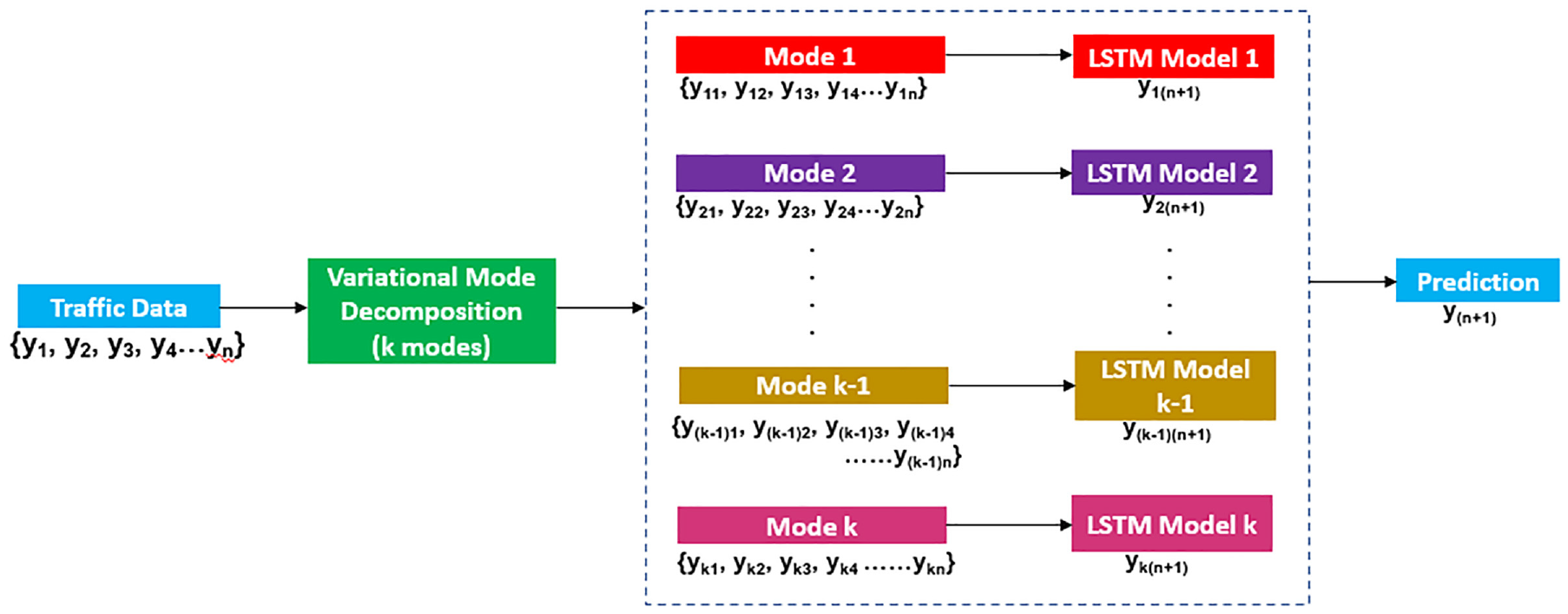
The present study focused on developing a hybrid deep learning model-based prediction framework to forecast the probability estimates of predicted travel time. This methodology integrated three different techniques—VMD, LSTM, and QR—to build a multi-input, single-output model while considering traffic flow and speed as inputs to predict travel time. Let $f (t) = y_{1}, y_{2}, y_{3} \dots y_{n}$ be the observations of the speed time series, and $g (t) = x_{1}, x_{2}, x_{3} \dots x_{n}$ the observations of the traffic flow time series. The speed time series was decomposed into multiple band-limited intrinsic mode functions (IMFs), as shown in Figure 1, using VMD, and dedicated LSTM models integrated with QR loss function were built for each of these modes to predict the upper and lower bounds of the predicted travel time. In addition, the decomposed signals were reconstructed to provide predicted travel time outputs. The following section briefs the background details of VMD, LSTM, and QR.

Figure 1.

Research schema.

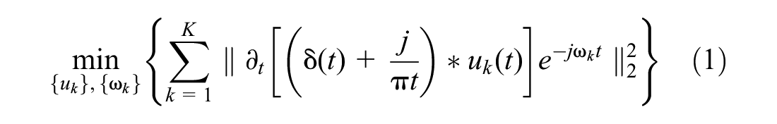
Variational Mode Decomposition

VMD is a nonrecursive signal processing method designed for decomposing complex nonstationary signals ( 20 ). The decomposition process is performed by a constrained variational problem to determine the bandwidth of each mode. This process involves three steps: 1) the Hilbert transform is used to obtain the unilateral frequency spectrum for each mode, 2) an exponential tuned to the estimated center frequencies is used to shift every mode’s frequency spectrum to baseband, and 3) the bandwidth of each mode is identified using the $H^{1}$ Gaussian smoothness of the demodulated signal. Thus, the constrained variational problem is defined as

min_{{u_{k}}, {ω_{k}}} {\sum_{k = 1}^{K} ∥ \partial_{t} [(δ (t) + \frac{j}{π t}) * u_{k} (t)] e^{- j ω_{k} t} ∥_{2}^{2}}

(1)

s . t \sum_{k = 1}^{K} u_{k} = f (t),

(2)

where

${u_{k}}$ is set of all modes,

${ω_{k}}$ is set of respective center frequencies,

$k$ is number of predefined modes,

$δ (t)$ is Dirac function,

j is an imaginary number. This is a complex valued analytic signal,

$* denotes$ a convolution, and

$∥ ∥_{2}^{2}$ denotes a squared $L^{2}$ -norm.

The present study adopted the number of predefined modes $(k)$ as 3, based on mode decomposition analysis. As suggested by Dragomiretskiy and Zosso, this constrained variational problem can be transformed into an unconstrained problem introducing a quadratic penalty term and Lagrangian multipliers, $λ$ , as follows ( 21 ):

\begin{matrix} L ({u_{k}}, {ω_{k}}, λ) = \\ α^{'} \sum_{k = 1}^{K} ∥ \partial_{t} [(δ (t) + \frac{j}{π t}) * u_{k} (t)] e^{- j ω_{k} t} ∥_{2}^{2} \\ + ∥ y (t) - \sum_{k = 1}^{K} u_{k} (t) ∥_{2}^{2} + 〈 λ (t), y (t) - \sum_{k = 1}^{K} u_{k} (t) 〉 \end{matrix}

(3)

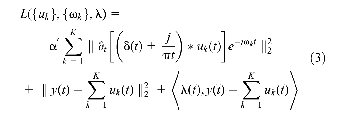
This equation can be solved using a sequence of iterative suboptimizations known as the alternate direction method of multipliers ( 22 , 23 ). By doing so, the modes, $u_{k}$ , and their respective center frequencies, $ω_{k}$ , are then updated simultaneously using the following expressions:

{\hat{u}}_{k}^{n + 1} (ω) = \frac{\hat{f} (ω) - \sum_{i \neq k} {\hat{u}}_{i} (ω) + \frac{\hat{λ} (ω)}{2}}{1 + 2 α^{'} {(ω - ω_{k})}^{2}}

(4)

w_{k}^{n + 1} = \frac{\int_{0}^{\infty} ω | {\hat{u}}_{k} (ω {) |}^{2} d ω}{\int_{0}^{\infty} | {\hat{u}}_{k} (ω {) |}^{2} d ω}

(5)

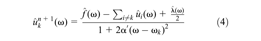
The modes are solved in the spectral domain and can be transformed back into the time domain by taking the real part of the inverse Fourier transform of the signal. In Equation 4, value $α^{'}$ represents a penalty term, defined by the user, which will define the shape of the modes.

Long Short-Term Memory

LSTM networks ( 24 ) regulate the flow of information using three gates (i.e., forget gate, $f_{t}$ ; input gate, $i_{t}$ ; and output gate, $o_{t}$ ), and a reservoir of long-term memory known as cell state, $c_{t}$ , to determine the hidden state, $h_{t}$ , of the network, which corresponds to the output determined at every time step (Figure 2). The following equations indicate how the information is transmitted through the network:

f_{t} = σ (W_{f} y_{t} + U_{f} h_{t - 1} + b_{f})

(6)

i_{t} = σ (W_{i} y_{t} + U_{i} h_{t - 1} + b_{i})

(7)

{\tilde{c}}_{t} = \tanh (W_{c} y_{t} + U_{c} h_{t - 1} + b_{c})

(8)

o_{t} = σ (W_{o} y_{t} + U_{o} h_{t - 1} + b_{o})

(9)

c_{t} = f_{t} ⊙ c_{t - 1} + i_{t} ⊙ {\tilde{c}}_{t}

(10)

h_{t} = o_{t} ⊙ \tanh (c_{t})

(11)

Firstly, the LSTM network decides whether the information from the previous time step is discarded or maintained by means of the forget gate, $f_{t}$ (Equation 6), where $x_{t}$ is the input; $h_{t - 1}$ the previous hidden state; $W_{f}$ and $U_{f}$ are the weights for the input and previous hidden state, respectively; $b_{f}$ the bias; and $σ$ represents a sigmoid activation function. The next step is to renew the information contained in the cell state, $c_{t}$ , based on the input and the previous hidden state, $h_{t - 1}$ . The new memory network is determined by the candidate cell state, ${\tilde{c}}_{t}$ (Equation 8), whereas the input gate, $i_{t}$ (Equation 7), acts as a filter to decide whether this new information is worth adding to the cell state, $c_{t}$ , or should otherwise be filtered. In these equations, $W_{c}$ and $U_{c}$ are the weights for the input and previous hidden state for the candidate cell state, ${\tilde{c}}_{t}$ ; $b_{c}$ the bias of the same candidate cell state, ${\tilde{c}}_{t}$ ; $W_{i}$ and $U_{i}$ the weights for the input gate; and $b_{i}$ the bias of the input gate. In this case, the candidate cell state uses a hyperbolic tangent as the activation function, whereas the input gate is activated with a sigmoid activation function.

Figure 2.

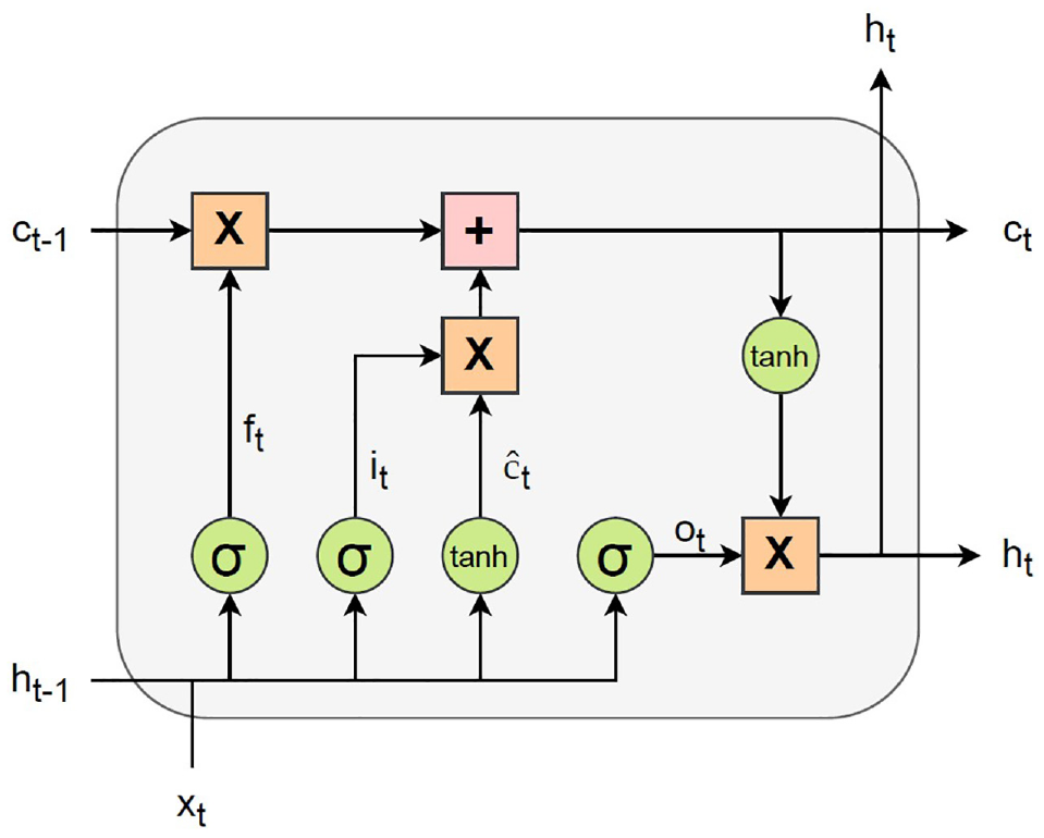
Structure of an LSTM network.

The cell state of the LSTM network is updated as shown in Equation 10, combining the elementwise product, $⊙, of$ the forget gate and the previous cell state with the elementwise product of the input gate and the candidate cell state ${\tilde{c}}_{t}$ . At this stage, the new hidden state h_t can be computed using the output gate (Equation 9) and the updated cell state of the network, as shown in Equation 11. The present study experimented with LSTM models under univariate and multivariate conditions.

Quantile Regression

In this study, we implemented a QR loss function—a nonparametric approach—to estimate the PI corresponding to the lower and upper boundaries of the estimate. PI is a measure illustrating the robustness of the algorithm in relation to its ability to quote the variation within an observed dataset. The loss function is equal to

ρ_{τ} (ϵ) = {\begin{matrix} τ ϵ, & if ϵ \geq 0 \\ (τ - 1) ϵ, & otherwise \end{matrix}

(12)

Then, the error function that must be minimized is

E_{τ} = \frac{1}{N} \sum_{i = 1}^{N} ρ_{τ} (y (i) - {\hat{y}}_{τ} (i))

(13)

where y(i) is the target value, and ${\hat{y}}_{τ} (i)$ is the forecast $τ$ -quantile.

Prediction and Performance Evaluation

In this study, the accuracy of point forecasts was quantified using the mean absolute percentage error (MAPE),

MAPE = \frac{1}{N} \sum_{i = 1}^{N} | \frac{y_{i} - {\hat{y}}_{i}}{y_{i}} | \cdot 100 %

(14)

where

N = number of samples,

$y_{i}$ = observations, and

${\hat{y}}_{i}$ = point forecasts.

However, the coverage and width of the PI must also be assessed for its evaluation. For that purpose, Prediction Interval Coverage Probability (PICP) metric was considered to measure the coverage of the PI and is defined as follows:

PICP = \frac{1}{N} \sum_{i = 1}^{N} c_{i}

(15)

where N accounts for the number of observations, and $c_{i}$ is equal to 1 if the observations fall within the PI, and 0 if not. A robust prediction algorithm would be expected to have a very high probability coverage.

The present study experimented with the aforementioned methodology in four ways (as shown in Table 1) to explore the best-performing combinations. Table 1 details the model combinations and their input variables adopted for prediction. Univariate models take past observations of speed time series as input to predict future values; multivariate models take past observations of both speed and flow time series as inputs to predict future speed values. Furthermore, VMD integrated models train dedicated LSTM models to predict values for each IMF, which are combined to obtain the final predicted speed signal.

Table 1.

Variations of Prediction Algorithms used for Travel Time Modeling

Serial no.	Models	Name	Inputs	No. of modes	Output
1	LSTM univariate	Uni-LSTM	Speed	NA	Travel time
2	LSTM multivariate	Multi-LSTM	Speed, Flow	NA	Travel time
3	VMD LSTM univariate	Uni-VMD-LSTM	Speed	3	Travel time
4	VMD LSTM multivariate	Multi-VMD-LSTM	Speed, Flow	3	Travel time

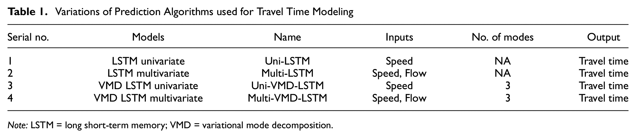
Note: LSTM = long short-term memory; VMD = variational mode decomposition.

Data Description

The data for this study were sourced from Traffic Infrastructure Ireland traffic counters ( 25 ) installed on the Irish road network. Vehicles are detected by passing over loops embedded beneath the road surface. Traffic counters provide information on the volume of traffic by time of day and by vehicle class (e.g., motorcycle, car, goods vehicles distinguished by the number of axles, etc.) with up to 12 classes being identified. In this study, we focused on six consecutive vehicle detectors located on the M50, the most prominent and busiest Irish motorway situated around the capital city, Dublin (see Figure 3). The M50 is a C-shaped, orbital, six-lane expressway corridor, with three lanes in each direction, that connects Dublin port with the M11 at Shankill, Ireland. All the other national routes radiate outwards from Dublin, their junctions beginning at the M50. The speed limit is 120 km/h and the traffic composition consists of 79.31% passenger cars, 0.2% motorbikes, 11.74% light goods vehicles, 7.89% heavy motor vehicles, 0.34% buses, and 0.525% caravans.

Figure 3.

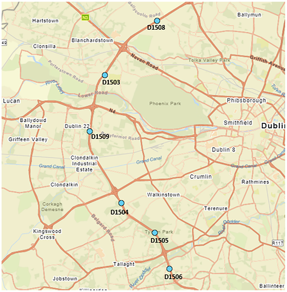
Map of test bed with the chosen detectors.

The raw data obtained were vehicle transactions consisting of time of passage, speed, vehicle type, and lane identifiers. For this study, the flow and speed values from the vehicle class “passenger cars” were considered for a period of 5 months (January to May 2019). Reserving the last month for testing (80:20 ratio), the remaining data were utilized for training and validation. The sourced data were processed in four stages: data cleaning, outlier removal, time series formation, and data imputation. Data cleaning involves extraction of the necessary information from the raw data, which consists of location-related details, lane identifiers, and vehicle identities such as tag-IDs and length, which were removed from the database to prepare the necessary inputs for the developed methodology. In the outlier removal stage, unreasonable data points that did not reflect the characteristics of the study sites were removed. Vehicle transactions with zero speed values, extremely high speed values of more than 200 km/h, and negative speed values were identified as outliers and removed from the database. Such values may have been incorrectly reported owing to sensor or communication errors.

In the next stage, the cleaned flow and speed values were processed to set up the time series. In the present study, the traffic flow and speed values observed at different times of the day were viewed as sequential data or a time series. The entire 24-h time window was divided into 5-min slots, such that we had twelve 5-min slots in an hour totaling 288 slots in a 24-h window. Further, the data were preprocessed such that at each time slot there was only one observation. In this regard, the traffic flow observation for any slot was the cumulative number of vehicles passing over the counter during a particular 5-min interval. The speed values were obtained by averaging the speeds of all the vehicles that passed over the counter during the 5-min period. Missing speed values resulting from there being no vehicles during a 5-min period were imputed by temporal substitution, in which temporally lagged observations were used for data imputation. Substitutions were designed based on the availability of data checked at different levels, such as an immediate past observation in time, and a week past observation, by taking advantage of the daily and weekly seasonality in the traffic data. This process of handling missing values is generally termed data imputation. The percentage of missing values was found to be less than 0.2% for the chosen dataset. The processed database comprised 43,488 observations in the continuous time series format with a 5-min resolution (frequency). A sample plot of processed speed and flow time series is shown in Figure 4. The descriptive statistics of the speed time series are clearly illustrated by boxplots presented in Figure 5.

Figure 4.

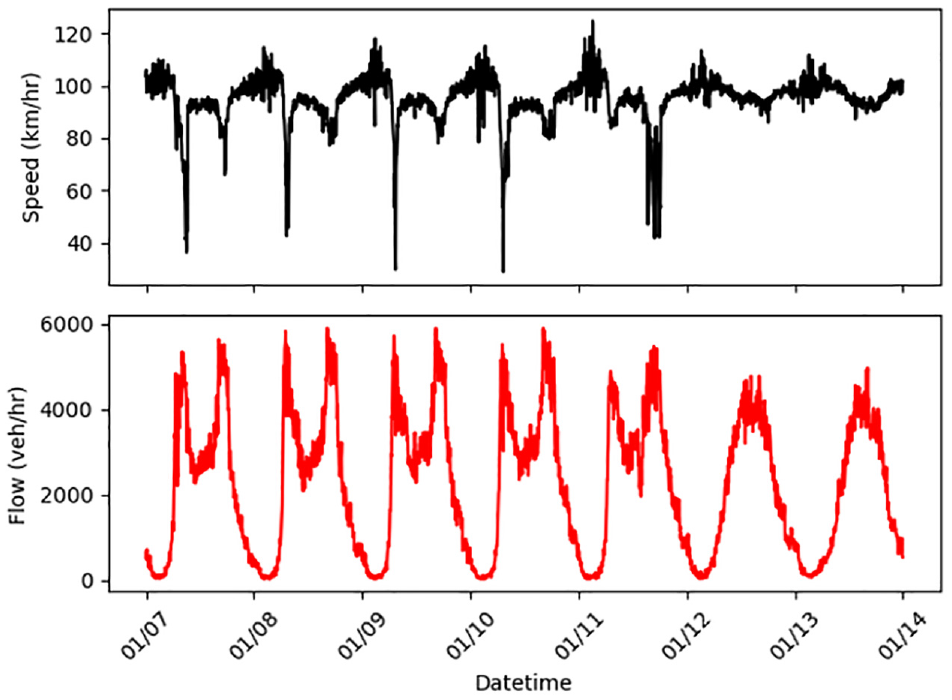
Sample plot of speed and flow time series.

Figure 5.

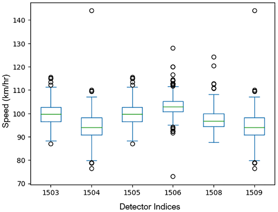
Box plot of speed sample across the considered detectors.

From Figures 4 and 5 it can be observed that the statistical characteristics of the speeds identified by each of the detectors were significantly different, despite being situated consecutively on the same motorway. On that note, Figures 4 and 5 collectively reflect the spatiotemporal variation in speed values observed on the M50. The processed speed time series was given as input to the developed variable mode decomposition algorithm, and three different band-limited IMFs (modes) were generated. A sample plot of the original speed signal and decomposed modes is shown in Figure 6.

Figure 6.

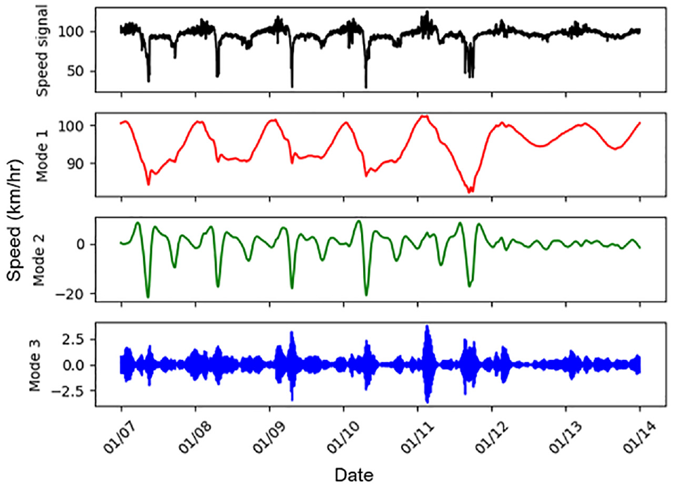
Mode decomposition of speed signal using VMD.

Further, each IMF was trained using dedicated LSTM models along with flow time series, and speed values were predicted. The present study considered 24 time-lagged observations to predict future travel time values with a 5-min horizon. In the subsequent stage, the travel time values were estimated from the predicted speed values.

Results

To explore the efficiency and performance of the developed model, the results were evaluated and compared against the benchmark models. To check the importance of the mode decomposition step during prediction, the performance of the VMD LSTM model was compared with a simple LSTM model, which takes the input without any preprocessing. To identify the advantages of considering traffic flow in travel time prediction, performances were compared between multivariate and univariate versions of the deep learning models. Overall, the four test cases (shown in Table 1) Multi-VMD-LSTM, Uni-VMD-LSTM, Multi-LSTM, and Uni-LSTM were considered and the prediction performances of all models compared.

Figure 7 shows the predicted travel time intervals of all the explored model combinations and measured travel times. It can be seen that intervals predicted by the multivariate models included all or most of the observed data points within the PIs, unlike the univariate models. It was also observed that the performance of the Multi-VMD-LSTM model was better than the other design variations, illustrating the advantage of adopting a signal processing tool like VMD when considering multiple variables. The VMD LSTM model presented a good adaptation to the data, even if some of the observations fall outside the interval.

Figure 7.

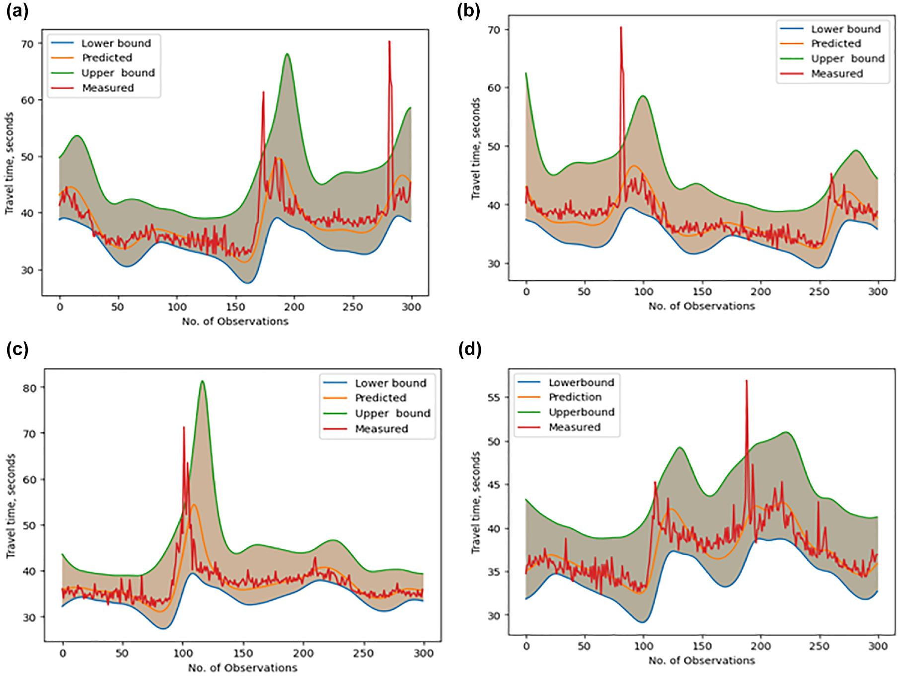
Prediction intervals across developed methods.

Figure 8 shows a comparison of PICP values across all the detectors among the four model variants. It was observed that the VMD LSTM model provided better coverage probability when compared with the LSTM models.

Figure 8.

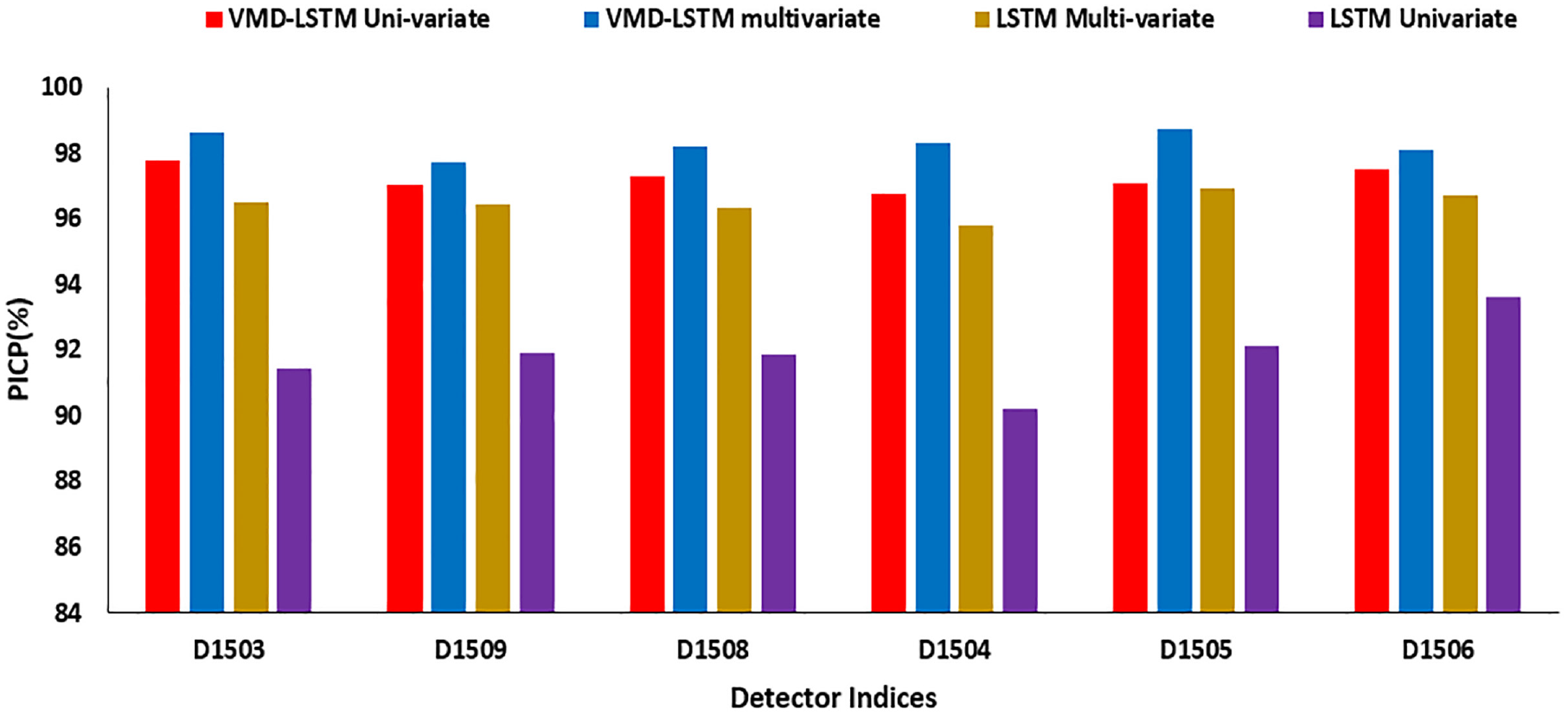
Comparison of PICP values across test detectors.

Further, the performance of all the modeled datasets considered in this study was compared to illustrate the consistency and effectiveness of the proposed methodology (Table 2). From the data presented in the table, it can be observed that the MAPE values of all the tested cases were between 3% and 6%. In the case of the six studied loop detectors, the VMD LSTM multivariate version of the proposed model outperformed the other models tested in this study. Preprocessing using the VMD proved to be the most useful addition to a conventional deep learning model such as LSTM. The use of both speed and flow in traffic prediction proved effective in the case of four detectors, whereas the other two did not show any effective improvement. This outcome was similar to model performance without the preprocessing step. Furthermore, preprocessing seemed to improve the impact of multivariate inputs.

Table 2.

Table of MAPE Values for all Test Cases

Detector ID	MAPE (%)
Detector ID	VMD LSTM multi-var	VMD LSTM uni-var	LSTM multi-var	LSTM uni-var
D1503	3.41	3.31	4.35	5.10
D1508	4.52	5.13	6.1	5.98
D1509	5.21	5.25	6.4	6.72
D1504	2.41	4.41	4.95	5.60
D1505	3.82	5.78	6.1	6.98
D1506	4.72	5.62	5.9	6.32

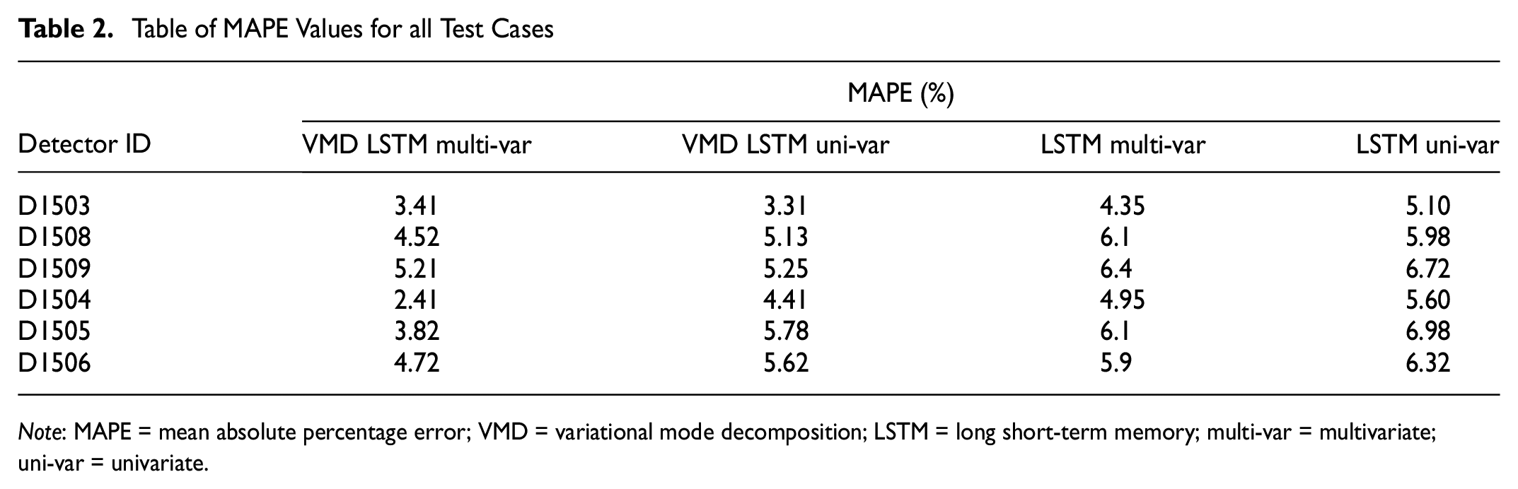
Note: MAPE = mean absolute percentage error; VMD = variational mode decomposition; LSTM = long short-term memory; multi-var = multivariate; uni-var = univariate.

Conclusion

Travel time prediction is essential to the developing and implementation of the majority of ITS applications in real time. The present study formulated a travel time prediction methodology by decomposing the input time series into multiple modes (IMFs) using VMD, and exclusive multivariate LSTM models were built for each of the IMFs, integrating QR to obtain the probabilistic intervals for the predicted travel time.

The probabilistic intervals produced the upper and lower bounds of the predicted travel time, providing a measure of uncertainty. Performance of the developed methodology was found to be efficient for both point forecasts, in which MAPE scores varied between 3% and 5%, and prediction intervals with PICP values varying between 97% and 99%. This performance was compared with simple LSTM models under univariate and multivariate cases to explore the advantages of a VMD–LSTM model combination. The results showed that the proposed method outperformed the benchmark methods in all cases, consistently showing the superiority of the developed methodology. Overall, the results showed that the VMD–LSTM–QR-based method was efficient and reliable for the purpose of travel time prediction. Furthermore, the probabilistic estimates around the point predictions (i.e., probabilistic prediction interval) acted as a measure of the robustness of the prediction algorithms and are essential for real-time implementations. Under unexpected traffic conditions during incidents, pandemics, and extreme weather events, PIs would be expected to provide meaningful bounds with which to understand the expected variations of travel time in the near future. The developed methodology would be completely transferable to any location with the availability of the aforementioned data source and initial training to learn about the model parameters. Further, the multivariate LSTM could be extended by adding suitable weather factors to develop a weather-adaptive travel time prediction system—a possible future extension to this study.

Footnotes

Author Contributions

The authors confirm their contribution to the paper as follows: study conception and design: D. Bharathi, J. M. González-Sopeña; data collection: D. Bharathi; analysis and interpretation of results: D. Bharathi; draft manuscript preparation: D. Bharathi, J. M. González-Sopeña, B. Ghosh, S. Clarke. All authors reviewed the results and approved the final version of the manuscript.

Declaration of Conflicting Interests

The authors declared no potential conflicts of interest with respect to the research, authorship, and/or publication of this article.

Funding

The authors disclosed receipt of the following financial support for the research, authorship, and/or publication of this article: This publication emanated from research supported in part by a grant from Science Foundation Ireland (grant no. 13/RC/2077P2).

ORCID iDs

Dhivya Bharathi

Juan Manuel González-Sopeña

Bidisha Ghosh

References

Williams

Hoel

Modeling and Forescating Vehicle Traffic Flow as a Seasonal Arima Process: Theoretical Basis and Empirical Results. Journal of Transportaion Engineering, Vol. 129, No. 6, 2003, pp. 664–672.

Bharathi

B. D.

Kumar

B. A.

Achar

Vanajakshi

Bus Travel Time Prediction: A Log-Normal Autoregressive (AR) Modelling Approach. Transportmetrica A: Transport Science, Vol. 16, No. 3, 2020, pp. 807–839.

Ghosh

Basu

Mahony

Multivariate Short-Term Traffic Flow Forecasting Using Time-Series Analysis. IEEE Transactions on Intelligent Transportation Systems, Vol. 10, No. 2, 2009, pp. 246–254.

Tirachini

Estimation of Travel Time and the Benefits of Upgrading the Fare Payment Technology in Urban Bus Services. Transportation Research Part C: Emerging Technologies, Vol. 30, 2017, pp. 239–256.

Wood

Gayah

Using Survival Models to Estimate Bus Travel Times and Associated Uncertainties. Transportation Research Part C: Emerging Technologies, Vol. 74, 2017, pp. 366–382. https://doi.org/10.1016/j.trc.2016.11.013.

Yin

Zhong

Zhang

Ran

A Prediction Model of Bus Arrival Time at Stops with Multi-Routes. Transportation Research Procedia, Vol. 25, 2017, pp. 4623–4636.

Chien

S. J.

Ding

Wei

Dynamic Bus Arrival Time Prediction with Artificial Neural Networks. ASCE Journal of Transportation Engineering, Vol. 128, No. 5, 2002, pp. 429–438.

Bin

Zhinzhen

Baozhen

Bus Arrival Time Prediction Using Support Vector Machines. Journal of Intelligent Transportation Systems, Vol. 10, No. 4, 2006, pp. 151–158.

Vanajakshi

Rilett

Support Vector Machine Technique for the Short Term Prediction of Travel Time. Proc., IEEE Intelligent Vehicles Symposium, Istanbul, Turkey, 2007, IEEE, New York, pp. 600–605.

10.

Agafonov

A. A.

Yumaganov

Bus Arrival Time Prediction Using Recurrent Neural Network with LSTM Architecture. Optical Memory Neural Networks, Vol. 28, 2019, pp. 222–230.

11.

Petersen

Rodrigues

Pereira

Multi-Output Bus Travel Time Prediction with Convolutional LSTM Neural Network. Expert Systems with Applications, Vol. 120, 2019, pp. 426–435. https://doi.org/10.1016/j.eswa.2018.11.028.

12.

Qin

Shao

Zhang

An Improved Bayesian Combination Model for Short-Term Traffic Prediction with Deep Learning. IEEE Transactions on Intelligent Transportation Systems, Vol. 21, No. 3, 2020, pp. 1332–1342. https://doi.org/10.1109/TITS.2019.2939290.

13.

Aloysius

Geetha

A Review on Deep Convolutional Neural Networks. Proc., International Conference on Communication and Signal Processing (ICCSP), Chennai, India, IEEE, New York, 2017. https://doi.org/10.1109/iccsp.2017.8286426.

14.

Huang

N. E.

Shen

Long

S. R.

M. C.

Shih

H. H.

Zheng

Yen

N.-C.

Tung

C. C.

Liu

H. H.

The Empirical Mode Decomposition and the Hilbert Spectrum for Nonlinear and Non-Stationary Time Series Analysis. Proceedings of the Royal Society of London. Series A: Mathematical, Physical and Engineering Sciences, Vol. 454, No. 1971, 1998, pp. 903–995.

15.

Huang

N. E.

Ensemble Empirical Mode Decomposition: A Noise-Assisted Data Analysis Method. Advances in Adaptive Data Analysis, Vol. 1, No. 1, 2009, pp. 1–41.

16.

Zheng

Pan

Pholsena

Mode Decomposition Based Hybrid Model for Traffic Flow Prediction. Proc., IEEE Third International Conference on Data Science in Cyberspace (DSC), Guangzhou, China, 2018, New York, IEEE, pp. 521–526.

17.

Tian

Approach for Short-Term Traffic Flow Prediction Based on Empirical Mode Decomposition and Combination Model Fusion. IEEE Transactions on Intelligent Transportation Systems, Vol. 22, No. 9, 2021, pp. 5566–5576. https://doi.org/10.1109/TITS.2020.2987909.

18.

Xiu

Sun

Peng

Chen

Learn Traffic as a Signal: Using Ensemble Empirical Mode Decomposition to Enhance Short-Term Passenger Flow Prediction in Metro Systems. Journal of Rail Transport Planning Management, Vol. 22, 2022, p. 100311.

19.

Sopeña

J. M. G.

Pakrashi

Ghosh

Interval Prediction for Short-Term Traffic Forecasting Using Hybrid Mode Decomposition Models. Proc., IEEE International Intelligent Transportation Systems Conference (ITSC), Indianapolis, IN, 2021, New York, IEEE, pp. 3246–3251.

20.

Sopena

J. M. G.

Pakrashi

Ghosh

Decomposition-Based Hybrid Models for Very Short-Term Wind Power Forecasting. Proc., 7th International Conference on Time Series and Forecasting, Gran Canaria, Spain, 2021.

21.

Dragomiretskiy

Zosso

Variational Mode Decomposition. IEEE Transactions on Signal Processing, Vol. 62, No. 3, 2013, pp. 531–544.

22.

Hestenes

M. R.

Multiplier and Gradient Methods. Journal of Optimization Theory and Applications, Vol. 4, No. 5, 1969, pp. 303–320.

23.

Boyd

Parikh

Chu

Distributed Optimization and Statistical Learning via the Alternating Direction Method of Multipliers. Now Publishers Inc., Delft, the Netherlands, 2011.

24.

Hochreiter

Schmidhuber

Long Short-Term Memory. Neural Computation, Vol. 9, No. 8, 1997, pp. 1735–1780.

25.

Traffic Counts/Data Map. 2013. https://trafficdata.tii.ie/publicmultinodemap.asp. Accessed March 15, 2022.

Travel Time Prediction Utilizing Hybrid Deep Learning Models

Abstract

Keywords

Methodology

Variational Mode Decomposition

Long Short-Term Memory

Quantile Regression

Prediction and Performance Evaluation

Data Description

Results

Conclusion

Footnotes

Author Contributions

Declaration of Conflicting Interests

Funding

ORCID iDs

References