Competition in Ride-Hailing Service Operations: Impacts on Travel Distances and Service Performance

Abstract

Competition in the ride-hailing market can influence traffic congestion and deteriorate the quality of service. A customer can request to be matched with a ride-hailing vehicle from their preferred company, which might not be the nearest vacant vehicle. This can increase both the customer’s matching and pick-up waiting time and the vehicle’s travel distance to the customer, and contribute to traffic congestion. Recent studies focus on the long-term competition effect by considering network equilibrium. In this work, we target a shorter timeframe and investigate how competition influences the passenger–driver matching process, the consequent vehicle travel to the customer, and more globally the system at the operational level. To this end, we propose a modeling and simulation framework based on the Macroscopic Fundamental Diagram (MFD). We apply the so-called M-model, a continuum approximation of the trip-based MFD. Compared with the accumulation-based approach, it explicitly monitors the remaining travel distance of all vehicles. We extend the mathematical M-model decomposition and focus on accurate dynamic estimation of trip lengths for the different vehicle states based on the immediate system state. For this, we suggest creating an additional proxy simulation framework replicating the demand requests and the service vehicle movements. We propose calibrating the matching function by sampling observations on a proxy grid network. Finally, we assess and compare different matching processes that define diverse competition scenarios: competition, cooperation, and competition with partial cooperation (coopetition). The cooperation scenario shows the best results in service performance.

This work is part of a global objective to investigate the advantages and drawbacks of competition within and between different transport modes or services. This topic has received little attention in scientific studies. Transportation companies often estimate the competition’s impact on other services with regard to their potential profit and losses. However, this approach is lacking an understanding of how competition influences urban, natural, and social environments. In this work, we focus on the competition between on-demand ride-hailing services. This choice is based on the behavior observation of ride-hailing companies in the US, where the recent emergence of the ride-hailing market has negatively contributed to network performance by increasing traffic congestion ( 1 ). Such services as Uber and Lyft increase their operating fleets to reduce customer waiting times ( 2 ), which creates extra congestion and consequently has a negative influence on CO₂ emissions as many vehicles move idly. Other countries have also experienced harmful externalities from competition between ride-hailing companies; for example, in China, it led to urban congestion and high emissions ( 3 ). Thus, we suppose that ride-hailing services contribute to traffic congestion not only by inefficient space usage (when a vehicle carries only one passenger) but also by fragmentation of the ride-hailing market. This means that a customer, instead of being served by the closest vacant car, chooses a vehicle of the most preferred or the cheapest company. Consequently, we conjecture that the distance an empty vehicle runs to pick up a customer increases in the oligopoly market compared with the monopoly scenario.

Most studies focus on the long-term effect of competition by considering network equilibrium ( 4 – 6 ). This permits assessment of the competition’s influence on fares, costs, demand rates, and other modeling parameters, some of which occasionally can be connected to our field of concern. Exploring competition includes a better understanding of the key factors that influence competition. Thus, some works are focused on governmental policies to regulate the competition of ride-hailing services with taxi ( 7 ) and public transport ( 8 , 9 ) alternatives. In this paper, we target a shorter timeframe and investigate how competition influences the passenger–driver matching process, the consequent vehicle travel for picking up the customer, and, more globally, the system at the operational level. It includes evaluating the system dynamics, congestion level, and service in the short term. Thus, we formulate the following research questions:

• How does competition during the matching phase influence service operations and network performances?

• What is the impact of different request distribution scenarios on service operations?

• How do fleet size, number of companies, and market share influence the competition outcome?

To respond to those questions, we propose a modeling and simulation framework. We decide to use the Macroscopic Fundamental Diagram (MFD) modeling framework for its simplicity and suitability to represent traffic dynamics at a large scale. The MFD connects the vehicle density with the mean network flow or speed. The related models are computationally efficient in predicting the aggregated traffic state dynamics ( 10 ). There are two main MFD types: accumulation-based and trip-based. In the accumulation-based model, the trip length is taken as an average and equal for all travelers. For the trip-based model, on the contrary, the trip length is individual for each traveler and is formulated as an integral of the network speed during the traveling period ( 11 ). As we study the behavior of on-demand services where there can be a significant variation in travel distance, especially when comparing steady and high-demand periods, the accumulation-based model is not the right choice because of the lack of detailed distance representation. In contrast, the trip-based model represents the travel distance of each trip. However, it is often computationally expensive to use this model. In our work, we use an intermediate approach named the M-model, a continuum approximation of the trip-based MFD model ( 12 ). Compared with the accumulation-based approach, it explicitly monitors the remaining travel distance of all vehicles and thus does not result in approximation of the mean distance traveled. We decompose the mobility service’s operations into several instances of the M-model. Each instance represents the different steps by conservation equations and depicts different vehicle states. Similar decomposition steps have been previously proposed by Beojone and Geroliminis ( 12 ). In this work, we extend the mathematical model decomposition and then focus on accurately estimating the trip lengths for the different steps. We assess and compare different matching processes that define diverse competition scenarios.

Competition Scenarios

We present three simulated scenarios to study the influence of competition on the services’ operations and system state. All scenarios have similar decision rules and cancelation policies, as described below.

Competition Between Companies

In this scenario, the companies operate in the system with no interaction except for sharing the same network speed for a given time. Each customer has a preferred company and cannot be served by another one. Each company defines a threshold of the idle distance a vehicle can travel to pick up a customer. For each passenger–vehicle match, the company looks for the idle distance to match this request. If the idle distance is less than the threshold then the customer is served by the assigned vehicle. Otherwise, the customer’s request is put in the waiting queue, and the vehicle stays vacant. If there are not enough vacant vehicles to serve a request, it is also put in the waiting queue. Demand requests wait in the queue for a pre-defined maximum time duration. If not matched in that time, the request is canceled.

Cooperation of Companies

We consider the cooperation scenario as that where any company can serve customers. In this case, the centralized system allocates a new demand request to the nearest vehicle if we assume that on-demand services have a similar pricing scheme. This assumption is reasonable at the market equilibrium as a company will lose customers to others if their fares are significantly different. The customer is served if the idle distance is less than a specific threshold. Otherwise, the request is put in the queue, and the vehicle remains vacant. Again, when there is a shortage of vacant vehicles, demand requests are put in the queue. If a demand request stays in the queue for more than the allowed time it is canceled.

Note that this scenario is similar to the monopoly market, as all the demand requests are put in the shared pool, and there is no distinction between different companies’ cars at the matching stage.

Competition with Partial Cooperation (Coopetition)

In this scenario, each customer has a preferred company. All the processes are similar to the previous two scenarios, including the comparison of idle distance for each matching with a threshold and putting customers with no assigned vehicles in the waiting queue. However, when the waiting time of a customer in the queue exceeds the allowed limit, this demand request is suggested to the rival company to be served. The other company then needs to decide based on the vehicle’s availability and the idle distance to this request. If there are no available vehicles or the idle distance to the request is longer than the allowed threshold, then the rival company refuses to serve the transferred demand and it is canceled. As the demand request distribution is made differently in these scenarios, their comparison can help to reveal the influence of competition and cooperation on the service operations.

The remainder of this paper is organized as follows. The next section presents the simulation modeling framework, including the state components and the calibration and integration of travel distance. The third section contains the simulation results, including the case study description, sensitivity analysis, and system dynamics representation. In the fourth and final section, the conclusion and future perspectives are presented.

Modeling Framework

State Components

This section presents the simulation modeling framework based on the M-model. First, we present the cycle of states through which each demand request and vehicle in the system passes. Three main actors are integrated into the modeling: users (demand requests), ride-hailing, and private vehicles. Their system states are represented in Figure 1a. The passengers have the following cycle. First, a demand request appears in the system. It can be put in the waiting queue or matched with a vehicle (matching decision-making). Note that the “waiting in a queue to be matched” user state is optional depending on the number of vacant vehicles and the idle distance to each demand. While waiting in the queue, a passenger can be matched with a new vacant vehicle (matching decision-making). After being matched, the passenger starts waiting for a vehicle to arrive. Then, the vehicle picks up the passenger, and they start to move together. The passenger onboard and an occupied ride-hailing vehicle are represented jointly in this state as their actions are identical. When the vehicle arrives at the destination, the cycle of the demand request is finished, and it is considered as served. The cycle of ride-hailing vehicles starts when a vehicle is idle and non-moving (vacant). If it is matched with a demand request, the idle vehicle starts moving to pick up a passenger. When it reaches the passenger, they start moving together till the demand destination is reached. After this, the vehicle becomes idle non-moving again. Private vehicle demand is served directly without waiting. The private vehicle moves with the passenger until the destination is reached and then disappears from the system. Thus, ride-hailing vehicles have three main states: idle non-moving (I), idle moving toward a passenger or simply idle moving (RHI), and occupied (RH). Private vehicles have only one state: a moving vehicle (PV).

Figure 1.

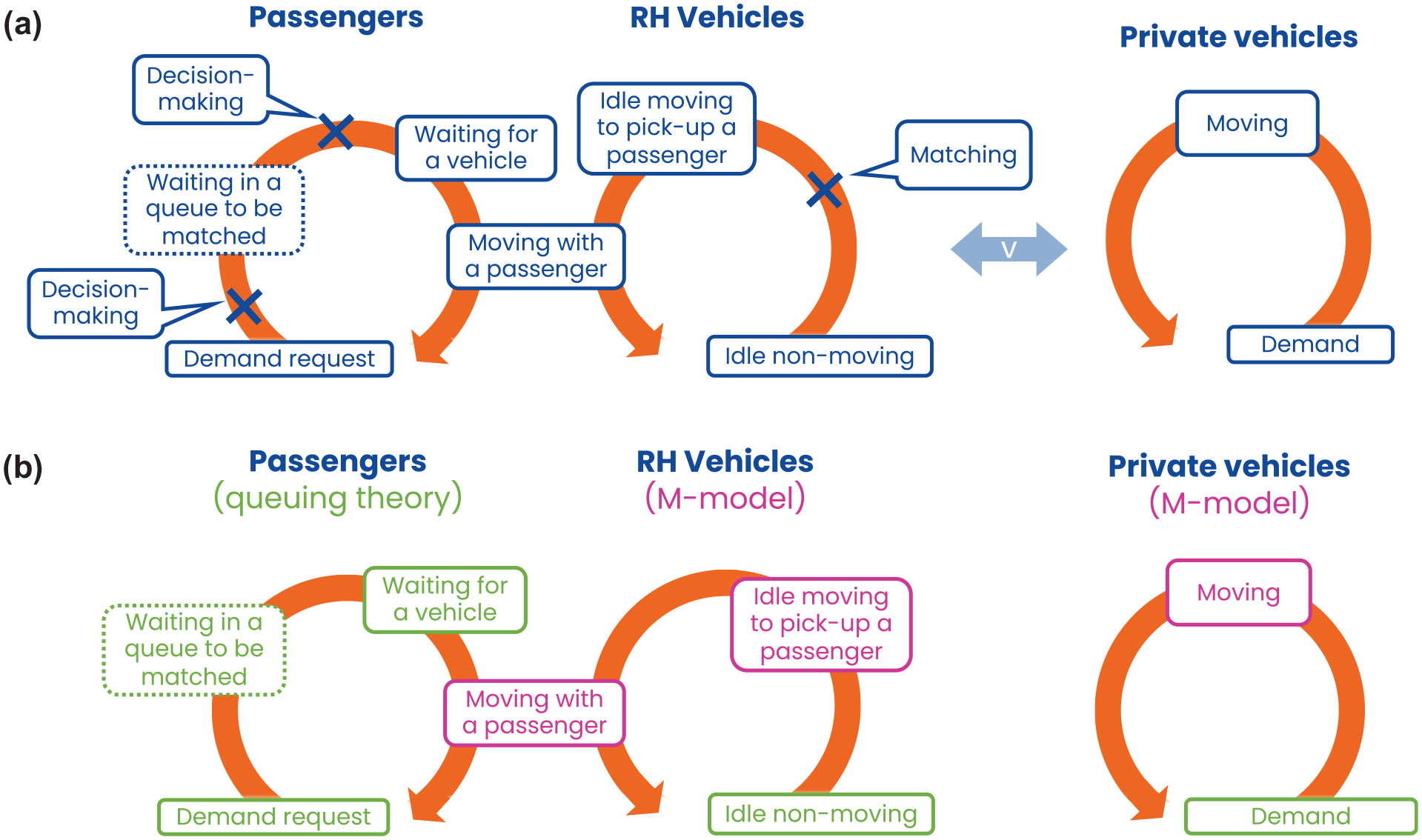
Diagram representing: (a) actors' states and decision-making and (b) actors' states processes using queuing theory and M-model.

In practice, after a drop-off, a vehicle can: (i) wait at the drop-off location, (ii) randomly drive (fishing), (iii) drive to a more attractive location (rebalancing), or (iv) drive to the new customer after a new match. In our setting, the vehicles only do (i) and then (iv), meaning that we consider the repositioning of the vehicles but only when they certainly know that they are matched with a customer. In this paper, we ignore the idle traveled distances from the random driving of vehicles before they receive a request. This cruising is not influenced by the level of competition (usually, a fraction of idle vehicles drive while waiting for a request). Considering such distance would certainly influence the traffic congestion as more vehicles driving reduces the speed. However, this will be affected by the total amount of ride-hailing vehicles and will not be changed based on how many companies are competing and their level of cooperation. As we focus on the influence of competition, we disregard this aspect. Note that smart rebalancing strategies using demand predictions or identifying more attractive areas would change this statement. However, this would require a complete description of the spatial dimension of the problem, which is not possible with the continuous description of the vehicle states we use. If we consider a perfect rebalancing, meaning that a vehicle can guess exactly where the next request will pop up, then, the travel distance is the same as the one we use, except that the trip will be made before the request appears. If the rebalancing is imperfect, extra distances are added but they are small compared with the overall relocation distance because otherwise the rebalancing is not effective. As the paper’s central focus is the competition between mobility providers, we believe that not considering rebalancing will not have a major impact on the results and its further analysis is beyond the scope of the paper.

Private and ride-hailing vehicles interact by sharing a common network speed. In an oligopoly market, several ride-hailing services participate in the simulation and share the same network speed.

When a vehicle or passenger enters the state marked in green in Figure 1b, they must wait before being served or matched. Such processes are well known in queueing theory when conservation of mass is guaranteed. These stages are represented by conservation equations considering inflows and outflows. The components corresponding to the driving phase (marked in pink in Figure 1b) are characterized by the M-model that defines the outflow depending on the remaining travel distances and the vehicle accumulation in the subsystems. Thus, the M-model reproduces the following vehicle states: private vehicles, idle moving ride-hailing vehicles, and occupied ride-hailing vehicles. The M-model assures not only the conservation but also helps to explicitly track the travel distance. Instead of having a steady-state outflow approximation of each vehicle state at every time step, we introduce transition phases related to the trip length dynamics. This approach helps to avoid the drawbacks of the travel distance representation in the accumulation-based MFD as it relaxes the steady-state approximation that defines the outflow. The list below summarizes the modeling framework notation:

$n^{\mathrm{PAS}}\left(t\right)$  = number of waiting passengers in a queue to be matched;

$n^I\left(t\right)$  = number of non-moving ride-hailing vehicles;

$n^{\mathrm{RHI}}\left(t\right)$  = number of idle moving ride-hailing vehicles to pick up a customer;

$n^{\mathrm{RH}}\left(t\right)$  = number of moving ride-hailing vehicles with a passenger on board;

$n^{\mathrm{PV}}\left(t\right)$  = number of private vehicles;

$M^{\mathrm{RHI}}\left(t\right)$  = total remaining distance of idle moving ride-hailing vehicles;

$M^{\mathrm{RH}}\left(t\right)$  = total remaining distance of moving ride-hailing vehicles with a passenger on board;

$M^{\mathrm{PV}}\left(t\right)$  = total remaining distance of private vehicles;

${\lambda }^{\mathrm{RH}}\left(t\right)$  = ride-hailing demand request arrival rate;

${\lambda }^{\mathrm{PV}}\left(t\right)$  = private vehicles demand request arrival rate;

$L^{\mathrm{RHI}}\left(t\right)$  = average trip length of an idle moving ride-hailing vehicle;

$L^{\mathrm{RH}}\left(t\right)$  = average trip length of a moving ride-hailing vehicle with a passenger;

$L^{\mathrm{PV}}\left(t\right)$  = average trip length of a private vehicle;

${\sigma }^{\mathrm{RHI}}\left(t\right)$  = standard deviation of $L^{\mathrm{RHI}}$ ;

${\sigma }^{\mathrm{RH}}\left(t\right)$  = standard deviation of $L^{\mathrm{RH}}$ ;

${\sigma }^{\mathrm{PV}}\left(t\right)$  = standard deviation of $L^{\mathrm{PV}}$ ;

$L_{\mathrm{RHI}}^{*}\left(t\right)$  = average remaining distance to be traveled by an idle moving ride-hailing vehicle in steady state;

$L_{\mathrm{RH}}^{*}\left(t\right)$  = average remaining distance to be traveled by a moving ride-hailing vehicle with a passenger in steady state;

$L_{\mathrm{PV}}^{*}\left(t\right)$  = average remaining distance to be traveled by a private vehicle in steady state;

$v\left(t\right)$  = average speed in the region;

$O^{\mathrm{RHI}}\left(t\right)$  = instantaneous trip completion rate for idle moving ride-hailing vehicles;

$O^{\mathrm{RH}}\left(t\right)$  = instantaneous trip completion rate for moving ride-hailing vehicles with a passenger on board;

$O^{\mathrm{PV}}\left(t\right)$  = instantaneous trip completion rate for private vehicles;

$O^{\mathrm{PAS}}\left(t\right)$  = matching rate of passengers with ride-hailing vehicles.

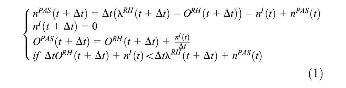
Equations 1 and 2 use the queueing theory to represent the relationship between the passenger queue accumulation $n^{\mathrm{PAS}}$ , the number of idle non-moving vehicles $n^I$ , and the matching rate $O^{\mathrm{PAS}}$ . The set of Equations 1 is valid when the demand exceeds the supply, while Equations 2 are true when there are enough vacant vehicles to serve the demand. Thus, Equations 1 and 2 represent the instances of the passenger waiting queue and idle non-moving vehicles. For the passenger queue, the inflow is the arriving demand, and the outflow is the matching result. The inflow of the idle non-moving vehicles instance are the vehicles that just finished delivering precedent passengers, and the outflow is the matching with a new demand, so this component is driven by a simple conservation principle.

$$\{\begin{array}{c}{n}^{\mathrm{PAS}}(t+\Delta t)=\Delta t({\lambda }^{\mathrm{RH}}(t+\Delta t)-O^{\mathrm{RH}}(t+\Delta t))-n^I\left(t\right)+n^{\mathrm{PAS}}\left(t\right)\hfill \\ \multicolumn{1}{c}{n^I(t+\Delta t)=0}\\ \multicolumn{1}{c}{O^{\mathrm{PAS}}(t+\Delta t)=O^{\mathrm{RH}}(t+\Delta t)+\frac{n^I\left(t\right)}{\Delta t}}\\ \multicolumn{1}{c}{\mathrm{if}\Delta t{O}^{\mathrm{RH}}(t+\Delta t)+n^I\left(t\right)<\Delta t{\lambda }^{\mathrm{RH}}(t+\Delta t)+n^{\mathrm{PAS}}\left(t\right)}\end{array}$$

(1)

or

$$\{\begin{array}{c}{n}^{\mathrm{PAS}}(t+\Delta t)=0\hfill \\ \multicolumn{1}{c}{n^I(t+\Delta t)=\Delta t(O^{\mathrm{RH}}(t+\Delta t)-{\lambda }^{\mathrm{RH}}(t+\Delta t))-n^{\mathrm{PAS}}\left(t\right)+n^I\left(t\right)}\\ \multicolumn{1}{c}{O^{\mathrm{PAS}}(t+\Delta t)={\lambda }^{\mathrm{RH}}(t+\Delta t)+\frac{n^{\mathrm{PAS}}\left(t\right)}{\Delta t}}\\ \multicolumn{1}{c}{\mathrm{if}\Delta t{O}^{\mathrm{RH}}(t+\Delta t)+n^I\left(t\right)\ge \Delta t{\lambda }^{\mathrm{RH}}(t+\Delta t)+n^{\mathrm{PAS}}\left(t\right)}\end{array}$$

(2)

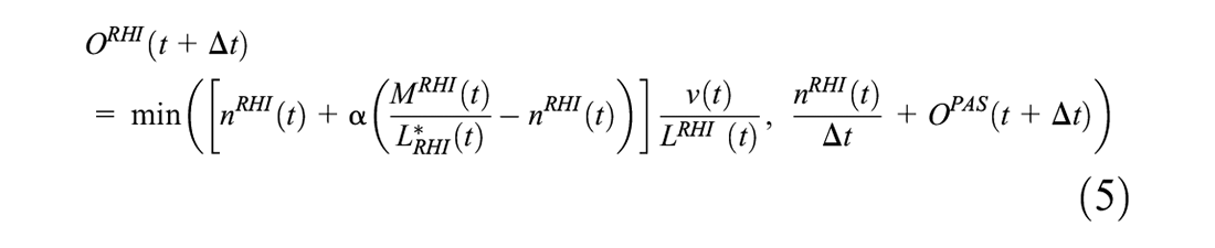
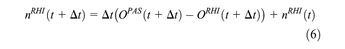
We group the equations according to the instance type (the state of vehicles) that they represent. Thus, Equations 5 to 7 represent the instance of idle moving vehicles $\mathrm{RHI}$ . Equation 5 represents the outflow calculated as the dynamic extension of the steady-state approximation. Recall that the steady-state approximation of the outflow is the production divided by the mean length $\frac{n^{\mathrm{RHI}}v}{L^{\mathrm{RHI}}}.$ However, if the trip length is heterogeneous, then during the transitional states the steady-state approximation can significantly vary from the real values. It is crucial, therefore, to account for the trip length dynamics. If in Equation 5 the term $\alpha =0$ , then the equation transforms into a steady-state approximation. Therefore, the term $\alpha (\frac{M^{\mathrm{RHI}}\left(t\right)}{L_{\mathrm{RHI}}^{*}\left(t\right)}-n^{\mathrm{RHI}}\left(t\right))$ of Equation 5 helps to capture the changes and represent the dynamics of the current trip length based on the total remaining distance and the average remaining steady-state distance.

We need to handle the situation when a vehicle state can become empty. This can occur if the outflow is higher than the inflow, leading to negative accumulation. To prevent this, we fix current accumulation in the corresponding vehicle state equal to zero

$$n^K(t+\Delta t)=\Delta t(O_{\mathrm{in}}^K(t+\Delta t)-O_{\mathrm{out}}^K(t+\Delta t))+n^K\left(t\right)=0$$

(3)

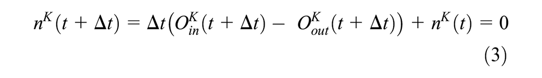
and obtain that

$$O_{\mathrm{out}}^K(t+\Delta t)=\frac{n^K\left(t\right)}{\Delta t}+O_{\mathrm{in}}^K(t+\Delta t)$$

(4)

where $K=\{\mathrm{RHI},\mathrm{RH},\mathrm{PV}\}$ , $O_{\mathrm{out}}^K$ is the outflow of the corresponding instance, and $O_{\mathrm{in}}^K$ inflow of the corresponding instance. Thus, when calculating the outflow at every time step, we need to take the minimum between the normal outflow value $[n^K\left(t\right)+\alpha (\frac{M^K\left(t\right)}{L_K^{*}\left(t\right)}-n^K\left(t\right))]\frac{v\left(t\right)}{L^K\left(t\right)}$ and the value of the negative accumulation case outflow $\frac{n^K\left(t\right)}{\Delta t}+O_{\mathrm{in}}^K(t+\Delta t)$ .

Equation 6 calculates the vehicle’s accumulation in state $\mathrm{RHI}$ , where the inflow is the matching result, and the outflow are the vehicles that just picked up their passengers. Equation 7 represents the total remaining distance of $\mathrm{RHI}$ vehicles. For each passenger–vehicle matching, the company looks for the idle distance $L^{\mathrm{RHI}}$ to match a specific request. The value of $L^{\mathrm{RHI}}$ is derived from the idle travel distance distribution considering the number of vehicles and the demand density. If the drawn idle distance is less than the pre-defined threshold then the customer is served by the assigned vehicle, otherwise, the demand request is put in the queue. The same process of drawing the distance from the distribution is used for other vehicle states, as we need to know the trip length of all new vehicles entering a new state. This is necessary to calculate the corresponding total remaining travel distance based on the trip length dynamics.

$$\begin{array}{c}{O}^{\mathrm{RHI}}(t+\Delta t)\hfill \\ =min([n^{\mathrm{RHI}}\left(t\right)+\alpha (\frac{M^{\mathrm{RHI}}\left(t\right)}{L_{\mathrm{RHI}}^{*}\left(t\right)}-n^{\mathrm{RHI}}\left(t\right))]\frac{v\left(t\right)}{L^{\mathrm{RHI}}\left(t\right)},\frac{n^{\mathrm{RHI}}\left(t\right)}{\Delta t}+O^{\mathrm{PAS}}(t+\Delta t))\hfill \end{array}$$

(5)

$$n^{\mathrm{RHI}}(t+\Delta t)=\Delta t(O^{\mathrm{PAS}}(t+\Delta t)-O^{\mathrm{RHI}}(t+\Delta t))+n^{\mathrm{RHI}}\left(t\right)$$

(6)

$$\begin{array}{c}\multicolumn{1}{c}{M^{\mathrm{RHI}}(t+\Delta t)=\Delta t(O^{\mathrm{PAS}}(t+\Delta t)·L^{\mathrm{RHI}}(t+\Delta t)}\\ \multicolumn{1}{c}{-n^{\mathrm{RHI}}(t+\Delta t)·v(t+\Delta t)}\end{array})+M^{\mathrm{RHI}}\left(t\right)$$

(7)

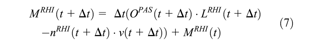
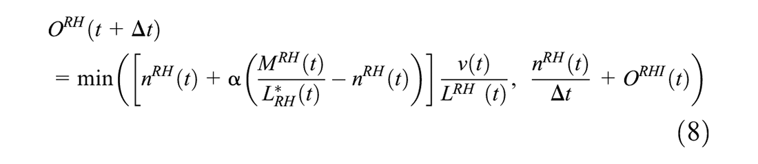
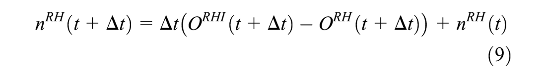
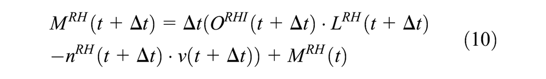
Equations 8 to 10 represent the occupied vehicles $\mathrm{RH}$ . Equation 8 stands for the outflow of this instance, that is, the vehicles that have delivered their passengers. Equation 9 calculates the vehicle accumulation in state $\mathrm{RH}$ where the inflow is the vehicles that have picked up passengers, and the outflow is the vehicles that have delivered passengers. The total remaining distance of $\mathrm{RH}$ vehicles is calculated using Equation 10.

$$\begin{array}{c}{O}^{\mathrm{RH}}(t+\Delta t)\hfill \\ =\min ([n^{\mathrm{RH}}\left(t\right)+\alpha (\frac{M^{\mathrm{RH}}\left(t\right)}{L_{\mathrm{RH}}^{*}\left(t\right)}-n^{\mathrm{RH}}\left(t\right))]\frac{v\left(t\right)}{L^{\mathrm{RH}}\left(t\right)},\frac{n^{\mathrm{RH}}\left(t\right)}{\Delta t}+O^{\mathrm{RHI}}\left(t\right))\hfill \end{array}$$

(8)

$$n^{\mathrm{RH}}(t+\Delta t)=\Delta t(O^{\mathrm{RHI}}(t+\Delta t)-O^{\mathrm{RH}}(t+\Delta t))+n^{\mathrm{RH}}\left(t\right)$$

(9)

$$\begin{array}{c}\multicolumn{1}{c}{M^{\mathrm{RH}}(t+\Delta t)=\Delta t(O^{\mathrm{RHI}}(t+\Delta t)·L^{\mathrm{RH}}(t+\Delta t)}\\ \multicolumn{1}{c}{-n^{\mathrm{RH}}(t+\Delta t)·v(t+\Delta t)}\end{array})+M^{\mathrm{RH}}\left(t\right)$$

(10)

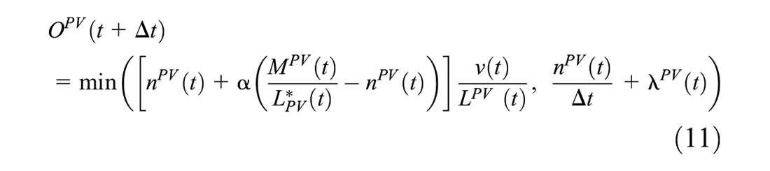
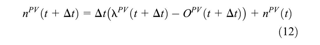
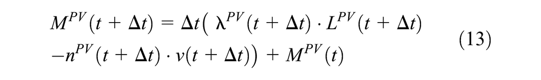
Equations 11 and 12 represent the private vehicles instance $\mathrm{PV}$ . Equation 10 calculates the outflow of the instance, that is, the vehicles that have finished their trips. Equation 11 calculates the private vehicle accumulation where the inflow is the demand, and the outflow is the vehicles that have finished travel. The total remaining distance of $\mathrm{PV}$ vehicles is calculated using Equation 10.

$$\begin{array}{c}{O}^{\mathrm{PV}}(t+\Delta t)\hfill \\ =\min ([n^{\mathrm{PV}}\left(t\right)+\alpha (\frac{M^{\mathrm{PV}}\left(t\right)}{L_{\mathrm{PV}}^{*}\left(t\right)}-n^{\mathrm{PV}}\left(t\right))]\frac{v\left(t\right)}{L^{\mathrm{PV}}\left(t\right)},\frac{n^{\mathrm{PV}}\left(t\right)}{\Delta t}+{\lambda }^{\mathrm{PV}}\left(t\right))\hfill \end{array}$$

(11)

$$n^{\mathrm{PV}}(t+\Delta t)=\Delta t({\lambda }^{\mathrm{PV}}(t+\Delta t)-O^{\mathrm{PV}}(t+\Delta t))+n^{\mathrm{PV}}\left(t\right)$$

(12)

$$M^{PV}\left(t+\Delta t\right)=\Delta t\left({\lambda }^{PV}\left(t+\Delta t\right)\cdot L^{PV}\left(t+\Delta t\right)-n^{PV}\left(t+\Delta t\right)\cdot v\left(t+\Delta t\right)\right)+M^{PV}\left(t\right)$$

(13)

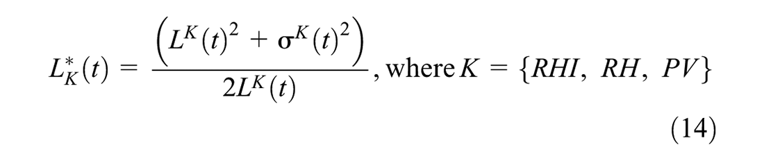
Equation 14 calculates the average remaining distance to be traveled in a steady state as a function of the average trip length and the standard deviation.

$$L_K^{*}\left(t\right)=\frac{(L^K{\left(t\right)}^2+{\sigma }^K{\left(t\right)}^2)}{2L^K\left(t\right)},\mathrm{where}K=\{\mathrm{RHI},\mathrm{RH},\mathrm{PV}\}$$

(14)

When several on-demand mobility services operate concurrently, it significantly affects the demand–supply matching process. Such a process is often represented by the Cobb-Douglas type meeting function ( 3 , 13 , 14 ), which was originally used in economics to model the relation between production output and inputs ( 15 ). For a set of $n$ inputs, the general form of the Cobb-Douglas function is

$$Y=f(x_1,x_2,\dots ,x_n)=\gamma \underset{i=1}{\overset{n}{\Pi }}{x}_i^{a_i}$$

(15)

where $Y$ is output, $x_i$ is input $i$ , and $\gamma$ with $a_i$ are parameters that determine the production’s general efficiency and the output’s sensitivity to input quantities changes ( 15 ). In transportation, this function calculates the matching rate based on the supply and demand quantities represented by the number of vacant vehicles and waiting passengers. Matching includes the time and distance required for a vehicle to reach a customer. The output can be expressed indifferently as matching rate, pick-up time, or idle travel distance to a customer. We would like to thoroughly explore the matching process between a passenger and a vehicle. In short, cooperation/competition between companies changes which vehicle can fit a travel request. The key factor is the distance between the customer and the matched vehicle. It depends on the demand density and its distribution among the companies and each company’s number of vacant vehicles.

In the modeling framework, it is important to represent the trip length of the vehicles in different states. The macroscopic modeling framework needs to be fed with individual trip lengths and to study trip length we need to look at the local matching process. The model requires not only the current mean value for both idle and occupied vehicle trip lengths but also its standard deviation. The general Cobb-Douglas meeting function requires calibration. Thus, it is important to approximate the idle trip length at each time step based on the immediate system state instead of using an average value for each trip. To do so, we suggest creating a proxy modeling framework that replicates the demand requests and the service vehicle’s movements. We propose calibrating the needed values using the Cobb-Douglas expression by sampling observations on a proxy grid network. Thus, by sampling multiple configurations, we can gain a full overview of the relation between trip lengths, demand levels, and vacant fleet sizes. We assume in the proxy that speeds are constant to keep computation time very low. This is crucial as we need to sample many configurations. Such a solution is faster than performing more computationally expensive simulations. This assumption affects travel distance which is a primary focus.

Note that different equations represent all driving states of vehicles, but they are all related to each other through the same network speed.

Modeling and Calibration of Travel Distance

In the proxy simulation, as we focus on distance traveled, speed and travel times are not the primary factors, so we assume that all vehicles move at the same speed during the sampling of observations and the demand is uniform.

The size of the grid network is chosen to be 7,000 × 7,000 m. Thus, the network surface is equal to 49 km², which is close to the area of Lyon (47.87 km²). The initial number of vehicles in the system and the number of requests that appear within each proxy simulation run are different in each run. In total, 200 proxy simulation runs are performed. This is done to diversify the possible system states that help identify the dependencies and factors that influence trip lengths. Note that we investigate idle trip length, that is, the travel distance required to pick up a customer, and the service trip length, that is, the travel distance with a customer on board. During each proxy run, the statistics about each trip are recorded to calculate the average values and standard deviation of different variables, for example, the distance run to pick up a customer, the number of vacant vehicles, and so forth. In the chosen matching strategy, the passengers follow the FCFS principle (first come, first served), but each demand request is assigned to the nearest vacant vehicle.

First, we study the vehicle travel distance with a passenger on board (service trip length or service distance). We notice that the variation in the service trip length is small regardless of the system’s saturation. Figure 2a shows the variation in the distance values experienced during the proxy simulation.

Figure 2.

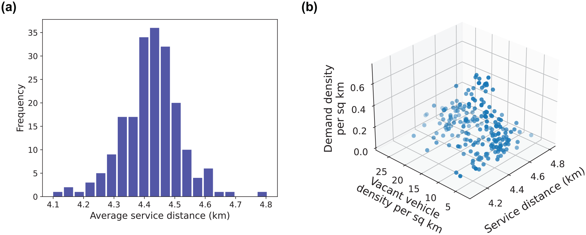
Vehicle travel distance with a passenger on board: (a) average service distance, (b) dependence of service distance on vacant vehicle density and demand density.

We want to investigate if system characteristics influence the service trip length. We test the influence of the density of demand requests appearing per time unit and the density of vacant vehicles. These two main parameters define the matching process according to the Cobb-Douglas meeting function. We use polynomial regression to show their influence on the service trip length. The regression shows no clear trend (coefficient of determination equal to 0.00514). The service trip length depends mostly on the demand pattern (OD pairs) and little on the service characteristics. OD pairs come from the same distribution, which does not depend on the number of vehicles, only on trips to perform that, consequently, depend on the network size. Figure 2b illustrates the dependence of the service distance on the density of demand requests and vacant vehicles, where no obvious trend is visible.

We will now investigate the idle trip length when the service is not saturated (i.e., no queueing of demand requests). Thus, the passengers still follow the FCFS principle and each demand request is assigned to the nearest vacant vehicle. Figure 3 shows the variation of the idle distance values experienced during the proxy simulation.

Figure 3.

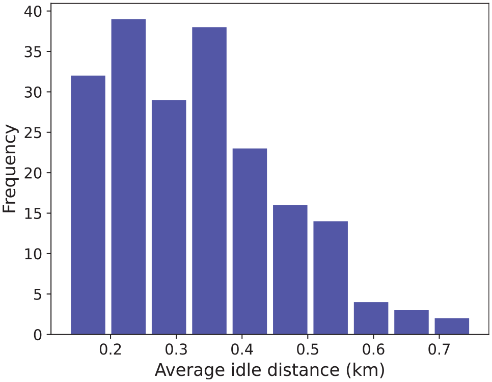
Average idle distance.

From Figure 3, we notice that the variation in idle distance is significant as the relative variation of idle distance is higher than the relative variation of service distance (Figure 2). Besides the demand pattern, it depends on other factors. We would like to investigate which system characteristics influence idle distance. We use polynomial regression to show the influence of the density of immediate demand requests and the density of vacant vehicles on idle distance. We obtain the coefficient of determination equal to 0.91. If we examine the dependence of idle distance on both parameters separately using polynomial regression, the obtained coefficient of determination is 0.88 for the vacant vehicle density and 0.011 for the demand density. The dependence of idle distance on those parameters is visualized in Figure 4, a to c .

Figure 4.

Dependence of idle distance on: (a) vacant vehicle density, (b) demand density, and (c) vacant vehicle density and demand density.

We observe the strong dependence of idle distance on the vacant vehicle density (Figure 4a). However, it also depends on the demand density, even though the relationship is less obvious. The region marked in green in Figure 4b is always empty. The reason is that if the demand density is high, it is easy for a vacant vehicle to have a request nearby, reducing the vehicle’s idle distance. The region marked in orange in Figure 4b is empty as the system does not reach the state where there are so many demand requests and vacant vehicles that the matched request and vehicle are situated very close to each other. Figure 4c illustrates the joint dependence of idle distance on vacant vehicle density and demand density.

Thereby, the Cobb-Douglas function expression is not explicit. The number of vacant vehicles and the demand rate influence the matching through the regression used to estimate the idle distance. Thus, it can be expressed as $L^{\mathrm{RHI}}\left(t\right)=F({\lambda }^{\mathrm{RH}}\left(t\right),n^I\left(t\right))$ , where $F\left(x\right)$ is the regression function.

We now consider the idle trip length of a saturated network, that is, where not enough vehicles are immediately available and passengers have to wait before being matched.

As long as there are not enough vehicles to serve all the demand requests, those requests enter a waiting queue. When a vacant vehicle appears, it serves the request with the longest waiting time in the queue. Thus, the passenger queue follows the FCFS principle. Previously, when the network was not saturated, each new request was assigned to the nearest vehicle. However, now with a shortage of vehicles and passengers waiting in a queue, each newly available vehicle is matched with the longest waiting passenger in the queue. This process can lead to two situations: (i) a single vacant vehicle becomes available; (ii) several vacant vehicles become available simultaneously.

Figure 5a shows the results of the proxy simulation when a single vacant vehicle becomes available and serves the first request in the queue. The idle distance distribution depicted in Figure 5a is for a city whose territory is 7 km in width and length. From Figure 5a, we see that the idle trip length follows a beta distribution with the parameters $\alpha =2.42,\beta =4.68$ , standard deviation $\sigma =2,323$  m, and mean value $4,710$  m. Thus, in the case of insufficient vehicle supply, the idle distance can be generated by knowing the parameters of the beta distribution.

Figure 5.

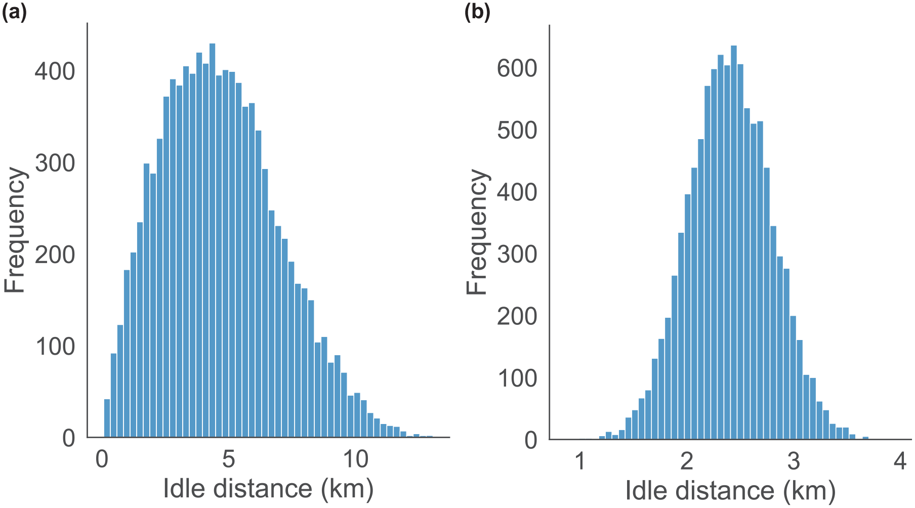
Idle distance distribution: (a) when single vacant vehicle becomes available and serves the first request in the queue and (b) when several vehicles become available simultaneously and the next request in the queue is served by the nearest vehicle.

When several vehicles become available simultaneously, we need to determine which vehicle will serve the subsequent request in the queue. The strategy used is for the nearest available vehicle to serve this demand. However, this process is not random and requires a proxy simulation to estimate the idle distance values. Based on the results from the proxy, the average standard deviation within this strategy is 386 m, and the average idle distance is 2,403 m, with the distribution depicted in Figure 5b. Thus, these values are used in the non-empty queue case.

Integration of Travel Distance into the Framework

To conclude, the distance is handled differently for each vehicle state. For the occupied vehicle state, the service trip length and its standard deviation are taken as an average from the proxy, as these values depend mainly on the network size. The same values are used for the private vehicles’ travel distance. In the situation of shortage of vacant vehicles, when new requests are put in a waiting queue, the idle distance of a vehicle and the standard deviation are taken as an average from the proxy. For idle vehicles without shortage of vacant vehicles, we show the dependency of the idle distance on the current demand rate and vacant vehicle density.

It is essential to highlight the integration of the travel distance sampling into continuous equations. The proxy simulation provides us with the distribution, that is, mean value and standard deviation, of trip length for all driving model components. At every time step when we either need to create new vehicles (PV case) or switch vehicles to a new state (ride-hailing case), we need to assign to these new vehicles a travel distance. This is done by sampling using the related distribution.

For Equations 7, 10, and 13, every time we add a new travel distance of vehicles in their new state, we summarize all the sample distances of the related vehicles. Knowing that the inflow is a continuous variable when we have a fractional number of vehicles, we draw and multiply the summarized distance by the fraction of vehicles.

Instead of tracking each vehicle individually (trip-based approach), we initialize the travel distance with the information obtained from proxy simulation and make it continuous. Thus, we make a trade-off between the trip- and accumulation-based approaches.

Thus, we use the proxy simulation to estimate the trip length for different values of demand rate and vacant vehicle density, then run polynomial regression to obtain the mean distance value and the standard deviation, and afterwards, do sampling to feed the M-model.

Simulation Results

Case Study Description

For the sake of simplicity, we choose the network characteristics to be similar to the network of Lyon, France. The general simulation parameters are the following. For all study cases, the time horizon is 4 h (14,400 s), with the 2 s time step of the system update. At each time step, the average speed $v\left(t\right)$ is calculated using speed functions of the Lyon metropolitan network from Balzer and Leclercq ( 16 ), where the variable is the number of all moving vehicles in the system (Figure 6).

Figure 6.

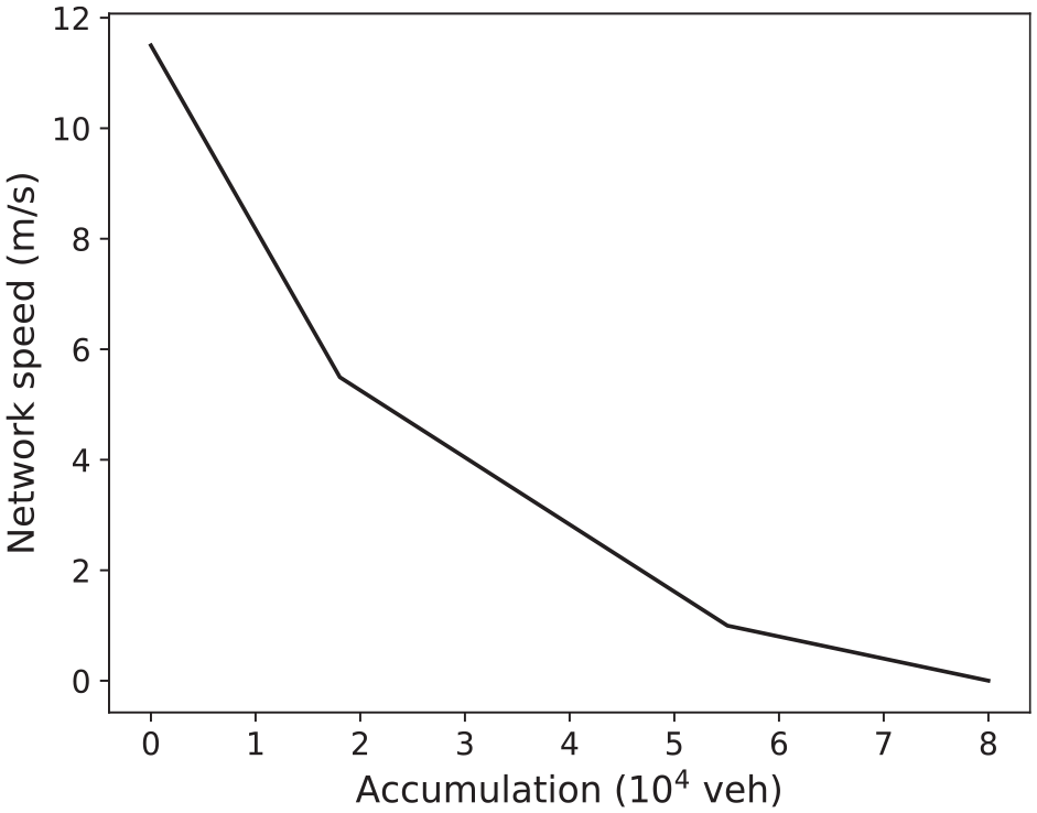
Network speed function.

The proportion of ride-hailing vehicles to the total number of vehicles should be consistent with the approximate percentage of vehicle miles traveled (VMT) by ride-hailing vehicles. Ride-hailing services in the US are responsible for between 1% and 14% of the total VMT ( 17 ). Erhardt et al. ( 1 ) claims that in San Francisco, ride-hailing trips constitute 15% of the overall number of vehicle trips. However, as the chosen network settings are based on the Lyon network characteristics, we decided to keep the number of ride-hailing vehicles consistent with this urban situation. The results of an additional study, where ride-hailing vehicles constitute 15%–17% of all the vehicles in the system, are presented in the supplemental material to this paper.

The demand rate benchmark is taken from Mariotte et al. ( 18 ), where the total vehicle demand during peak hours is around 25–27 vehicles per second. Applying the ratio of ride-hailing vehicles/private vehicles to the demand, it is possible to calculate the demand rate for each mode.

To test the system reaction based on the demand changes, for ride-hailing and private vehicles the demand value is set to be uniform at each time step during a certain period, then it starts to increase, reaches its peak, and consequently decreases to the original value, and remains constant till the end of the simulation (Figure 7, a and b ).

Figure 7.

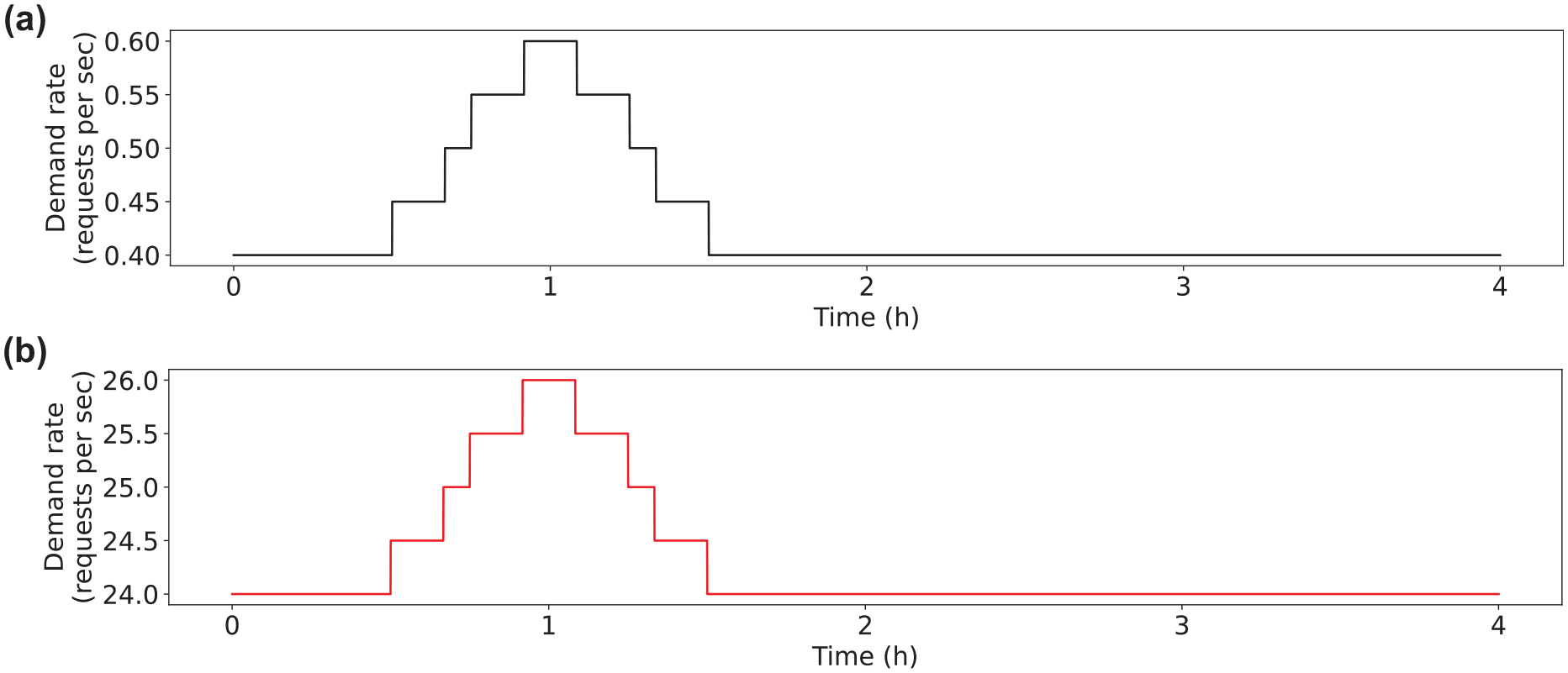
Demand curve for (a) ride-hailing vehicles and (b) private vehicles.

As mentioned above, the service travel distance depends mainly on the network size. Thus, using the proxy simulation, we obtain the average value of 4,424 m and its standard deviation of 60 m for the given network size. We also assume these parameters are valid for private vehicle journeys. Thus, for each vehicle–passenger pair and each private vehicle, we draw a service travel distance using the mentioned parameters and considering the normal distribution.

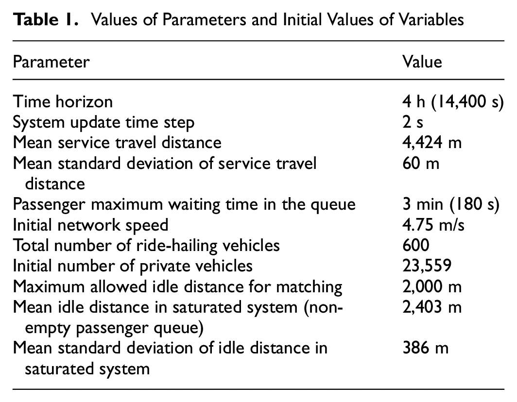
Consider the allowed waiting time in the queue to be 3 min, and the allowed threshold of idle vehicle distance is 2,000 m. The simulation’s initial values are the following. To investigate the system’s behavior close to the saturation state, we set the initial system speed to 4.75 m/s. The total initial number of vehicles in the system should be consistent with the network speed and can be calculated using the MFD curves ( 16 ). Thus, based on the corresponding calculations, we obtain the initial number of private vehicles equal to 23,559 and the total number of ride-hailing vehicles equal to 600. Knowing the demand, this ratio leads to the ride-hailing service being responsible for 2%–3% of the total VMT. The initial value of the total remaining distance for each vehicle state is calculated assuming each vehicle has left to run half of the respective distance on average. The summary of parameter values and initial values of variables is shown in Table 1.

Table 1.

Values of Parameters and Initial Values of Variables

Parameter	Value
Time horizon	4 h (14,400 s)
System update time step	2 s
Mean service travel distance	4,424 m
Mean standard deviation of service travel distance	60 m
Passenger maximum waiting time in the queue	3 min (180 s)
Initial network speed	4.75 m/s
Total number of ride-hailing vehicles	600
Initial number of private vehicles	23,559
Maximum allowed idle distance for matching	2,000 m
Mean idle distance in saturated system (non-empty passenger queue)	2,403 m
Mean standard deviation of idle distance in saturated system	386 m

Sensitivity Analysis

To evaluate how the competition during the matching phase and different request distribution schemes influence service operations and network performance, we compare the metrics of cooperation, competition, and coopetition scenarios given the same initial parameters for each of them. To evaluate the output of different settings, we implement the following test cases: variation of the ride-hailing market fleet size, the number of companies in the system, the market share of ride-hailing and private vehicles, the variation of fleet size between the companies within the ride-hailing market, and the variation of demand share between the companies within the ride-hailing market. To find the outcome of different scenarios, we compare the percentage of canceled demand and the average passenger waiting time for being matched. We do not discuss the influence of the considered scenarios on the network speed, as in the considered settings that correspond to the state of the city of Lyon the penetration rate of mobility services is low and does not have a strong influence on the system. Thus, the variation in speed is minimal, as shown in the “System Dynamics for the Reference Scenario” subsection. For the test case where the penetration rate of ride-hailing mobility services is higher (15%–17% of market share), the results are presented in the supplemental material to this paper., including the network speed analysis. From that analysis, we can see that with the increased number of ride-hailing vehicles in the system, the best network performance is observed for the cooperation scenario, closely followed by coopetition. In the case of competition, the network speed deteriorates significantly compared with the other two scenarios.

Ride-Hailing Market Fleet Size

To see the impact of different fleet sizes, we vary the number of vehicles of each company and compare the metric values while keeping the same demand rate. Considering that the benchmark number of ride-hailing vehicles in the system is equal to 600 (270 for Company 1 and 330 for Company 2), we change this number in the following way: 660 vehicles (+10% of the benchmark number, 297 and 363 respectively), 540 vehicles (−10% of the benchmark number, 243 and 297 respectively), and 480 vehicles (−20% of the benchmark number, 216 and 264 respectively). The results are shown in Figure 8, a to c .

Figure 8.

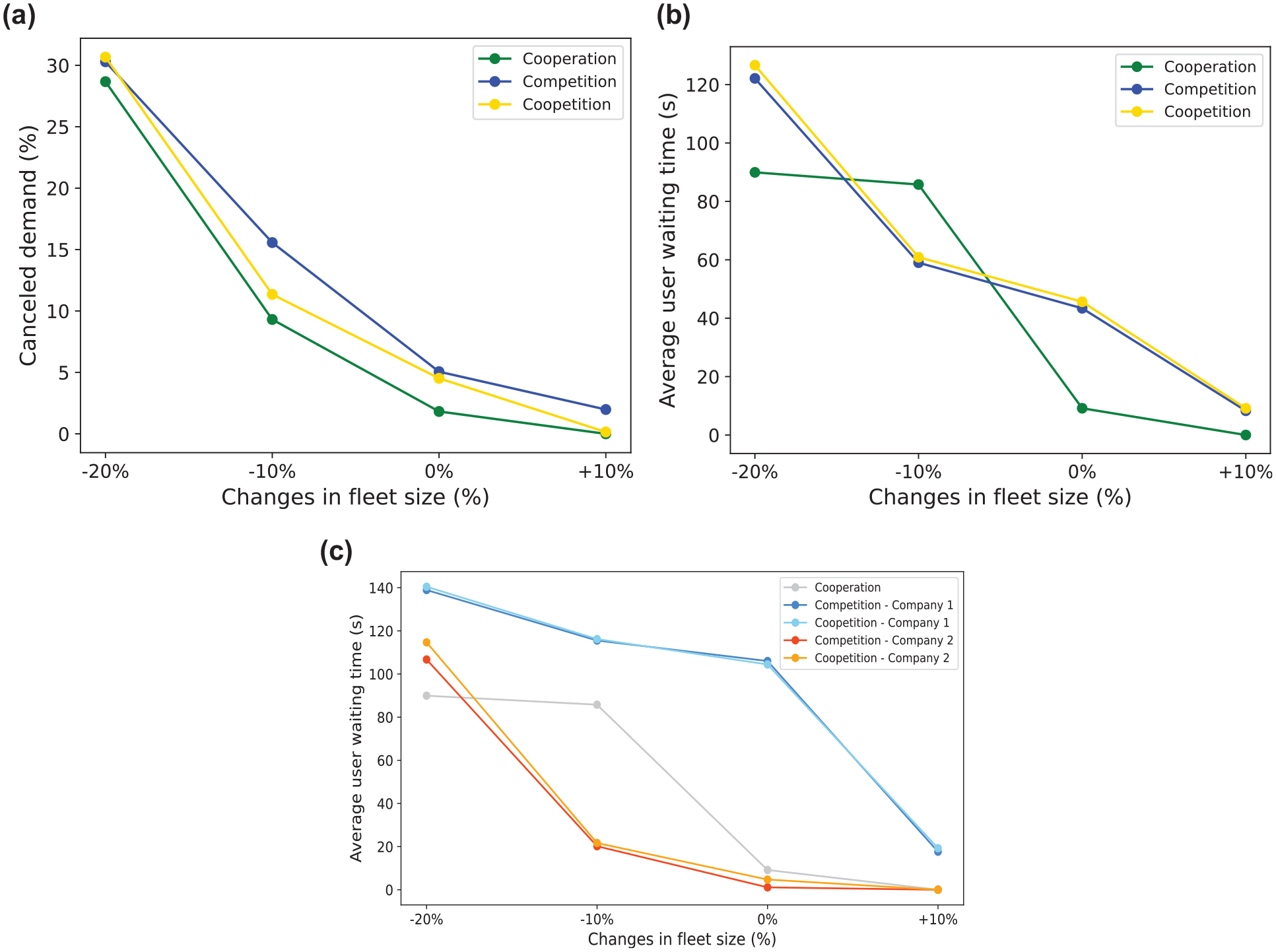
Different fleet sizes: (a) percentage of canceled demand, (b) average passenger waiting time to be matched, and (c) average passenger waiting time to be matched by company.

Figure 8a depicts the common decrease of canceled demand among all the test cases with the increase in fleet size. The competition case has a higher cancelation rate, followed by coopetition and cooperation.

Figure 8b shows that the average passenger waiting time decreases with increase in the fleet size for all the scenarios. Generally, the average waiting times of the competition scenario and the coopetition are close and follow the same curve (the waiting time for competition is slightly smaller). In the cooperation scenario, most of the time, the waiting time is shorter than in the competition and coopetition scenarios for the cases of −20%, 0, and +10% fleet size changes. However, for the case of −10% fleet change, the waiting time of cooperation surpasses other scenarios. The reason is the following. In the competition scenario, the cancelation rate is higher than in cooperation; therefore, the vehicles need to serve fewer customers. Thus, the availability rate of vehicles is higher, so the waiting time of the passengers is less. On the contrary, the cooperation scenario reaches a stable state where a customer from the queue is served just before being potentially canceled. Thus, fewer requests are canceled, but the passenger waiting time is higher. At the same time, in both the coopetition and competition scenarios, the low average waiting time is guaranteed because Company 1 (with fewer vehicles) has a stably big queue of requests while Company 2 (with more vehicles) has a queue for a relatively short time, which leads to a shorter average waiting time for customers in the system. This statement is supported by Figure 8c.

Figure 8c shows how different scenarios affect the quality of service operations of an individual company by comparing the average company’s passenger waiting time. For Company 1, which has fewer vehicles than Company 2, the average passenger waiting time does not differ significantly in the competition and coopetition scenarios. For Company 2, the competition scenario has a slightly shorter waiting time than for coopetition. The reason is that in coopetition Company 2 serves its rival’s customers. Thus, Company 2 runs out of vacant vehicles faster than in the competition scenario, leading to a longer waiting time for their own customers. There is no big difference between the waiting time of the competition and coopetition for both companies, as the customers that reach the waiting limit in the cooperation scenario will be transferred to the rival company instead of being canceled, which results in the same waiting time for them.

Number of Companies

To study the impact of an oligopoly market, we implement and compare test cases with two, three, and four companies (Figure 9, a and b ). The number of vehicles of each company in the test cases is the following. For the two-company market, Company 1 has 270 vehicles and Company 2 has 330 vehicles. For the three-company market, Company 1 has 200 vehicles, Company 2 has 220 vehicles, and Company 3 has 180 vehicles. For the four-company market, Company 1 has 175 vehicles, Company 2 has 165 vehicles, Company 3 has 135 vehicles, and Company 4 has 125 vehicles. The demand is equally distributed among all the companies. In the figures, we include the results of the cooperation scenario to compare them with oligopoly cases. The number of vehicles in the cooperation scenario is 600.

Figure 9.

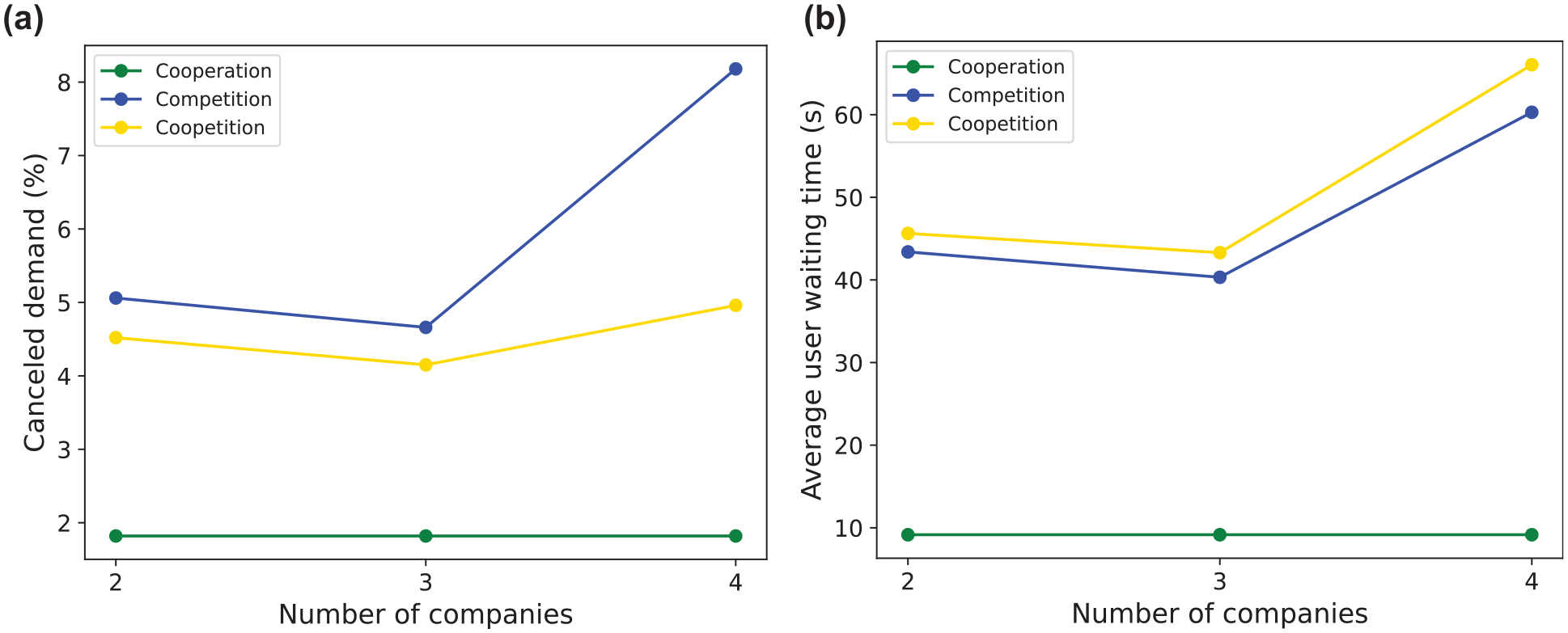
Number of companies: (a) percentage of canceled demand and (b) average passenger waiting time to be matched.

Figure 9a shows that the average percentage of canceled demand in the competition and coopetition scenarios slightly decreases for the three-company market compared with the two-company market, and then increases for the four-company market. The cancelation rate is the highest for the competition scenarios, less for coopetition, and the smallest for the cooperation system.

Figure 9b depicts that the average passenger waiting time slightly decreases for the three-company market compared with the two-company market, and then increases for the four-company market in the competition and coopetition scenarios. The longest passenger waiting time is experienced in the coopetition scenario because vacant vehicles of one company need to serve the customers of the rival company. This imposes a longer waiting time for the customers of the former company because of the higher occupancy of vehicles. The shortest waiting time is experienced in the cooperation scenario.

Market Shares of Ride-Hailing and Private Vehicles

In this section, we test different market shares, that is, when some demand for private vehicles moves to ride-hailing and the vehicles themselves. The demand is distributed equally between both companies. Thus, we increase the ride-hailing demand and fleet size by 30% and 50% while reducing those parameters for private vehicles. The benchmark number of ride-hailing vehicles in the system is 600, and we increase it by 30% (780 vehicles) and 50% (900 vehicles). For the two-company market, the benchmark number of vehicles equals 270 for Company 1 and 330 for Company 2. Those numbers increase respectively by 30% and 50%. The results are presented in Figure 10, a to c .

Figure 10.

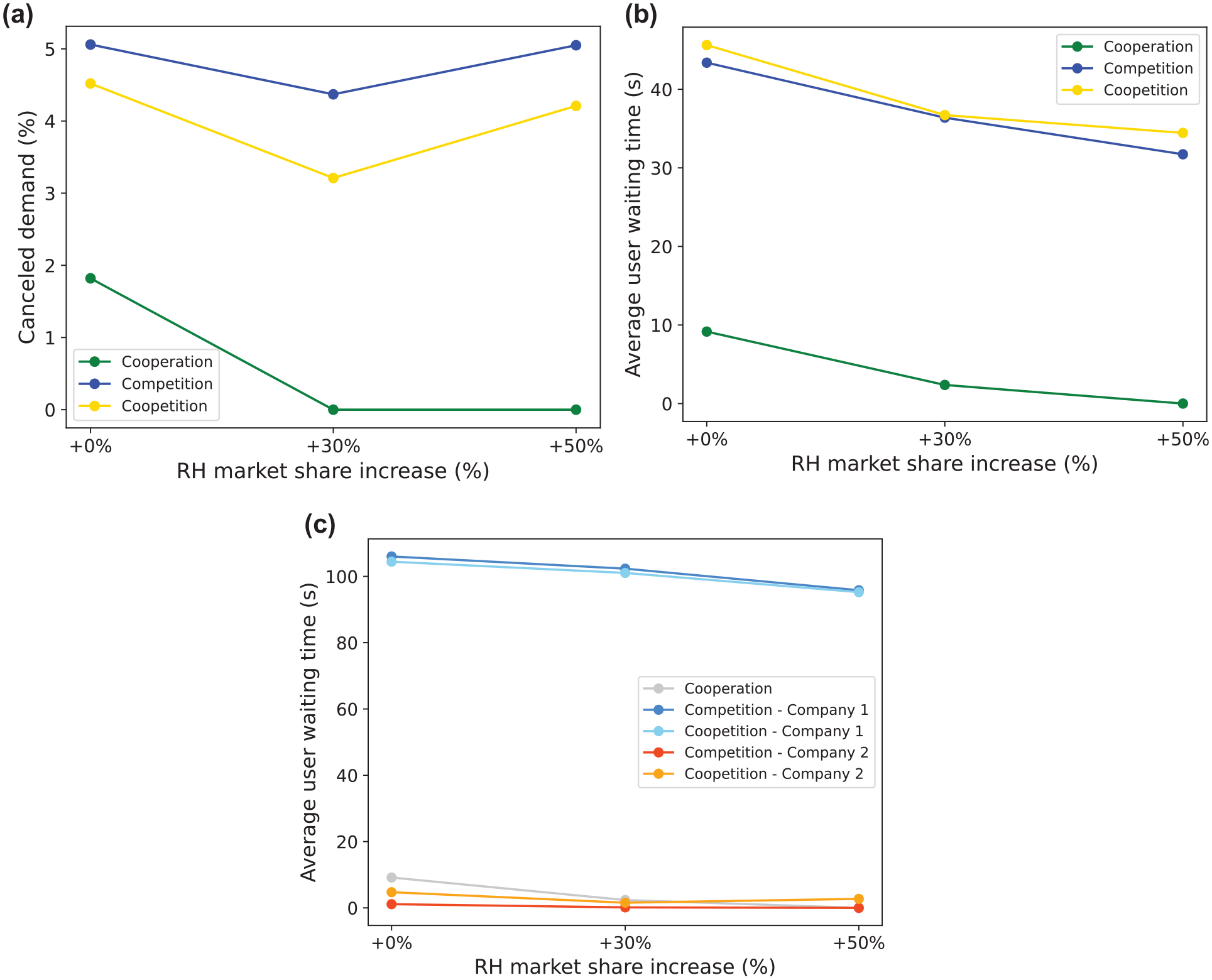
Different market shares of ride-hailing and private vehicles: (a) percentage of canceled demand, (b) average passenger waiting time to be matched, and (c) average passenger waiting time to be matched by company.

Figure 10a shows that the percentage of canceled demand decreases for all scenarios for the +30% market share, and then increases for the competition and coopetition scenarios for the +50% market share. The highest cancelation rate is in the competition scenario, then in coopetition, and the smallest is in the cooperation scenario.

Figure 10b shows that the average passenger waiting time decreases with rail-hailing market share increase for all the scenarios. The longest waiting time is experienced in the coopetition scenario as, compared with competition, some passengers that reach the waiting time limit are transferred and served by another company. This increases the overall occupancy rate of vehicles in the system and imposes a longer waiting time. A slightly shorter waiting time is experienced in the competition scenario. The shortest waiting time is in the cooperation scenario as it serves the passengers optimally.

Figure 10c depicts how different scenarios affect the quality of service operations of an individual company. In Company 1, which has fewer vehicles than Company 2, the average passenger waiting time does not differ significantly in the competition and coopetition scenarios. For Company 2, the coopetition scenario has a longer waiting time than the competition. Both curves of Company 2 are very close to the curve of the cooperation scenario.

Fleet Share Between Companies Within the Ride-Hailing Market

To see the impact of different fleet sizes of companies within the ride-hailing market, we vary the number of vehicles of each company while keeping the same total number of ride-hailing vehicles in the system. We compare the metric values while keeping the usual demand rate. Considering that the total number of ride-hailing vehicles in the system is equal to 600, we vary the fleet share in the following way: 255 and 345 vehicles of correspondingly to Company 1 and Company 2, 270 and 345 vehicles, 285 and 315 vehicles, and 300 and 300 vehicles. The results are shown in Figure 11, a to c .

Figure 11.

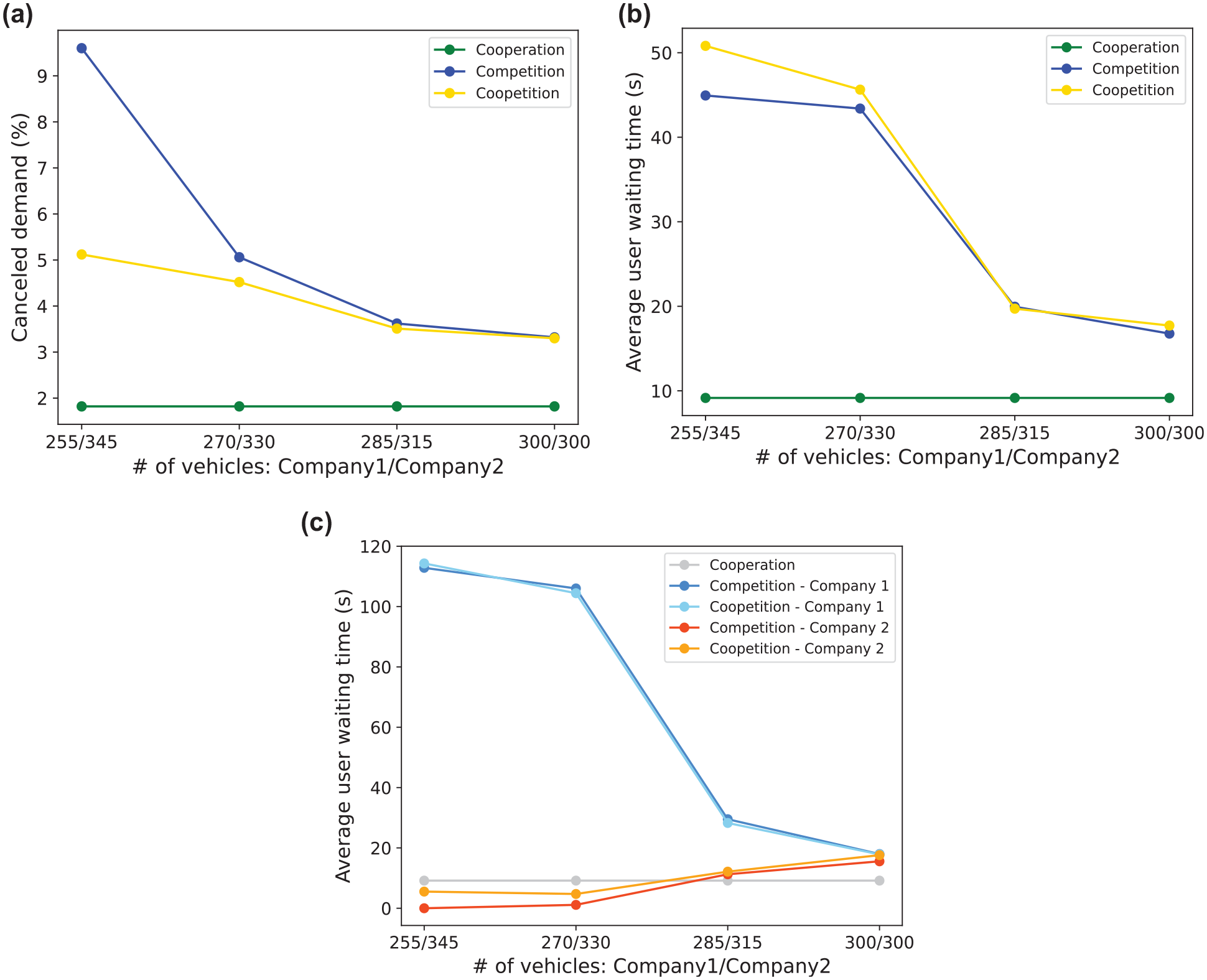
Different fleet sizes of ride-hailing companies: (a) percentage of canceled demand, (b) average passenger waiting time to be matched, and (c) average passenger waiting time to be matched by company.

Keeping in mind that the companies share the ride-hailing demand equally, Figure 11a shows that as the number of vehicles of both companies approaches equality, the number of canceled demand requests reduces correspondingly and reaches the same level. At the same time, as the number of vehicles approaches the equal division between the companies, the overall waiting time of passengers decreases (Figure 11b) as the system approaches the optimal redistribution of the supply according to the demand. It is also visible in Figure 11a that the most significant variation in demand cancelation occurs under the competition scenario compared with the coopetition scenario.

Figure 11c depicts how the equilibration of the supply decreases the waiting time of the users of Company 1 and subsequently increases the waiting time of the users of Company 2, which leads to equality between the two companies.

Demand Share Between Companies Within the Ride-Hailing Market

In this section, we test different demand shares of companies within the ride-hailing market. We vary the demand rates of each company while keeping the same total number of ride-hailing demand in the system. Considering the demand rate shown in Figure 8a as the benchmark for both companies, we decrease the demand level for Company 1 by 25% and 50% and correspondingly increase the demand level for Company 2 by 25% and 50%. The results are presented in Figure 12, a to c .

Figure 12.

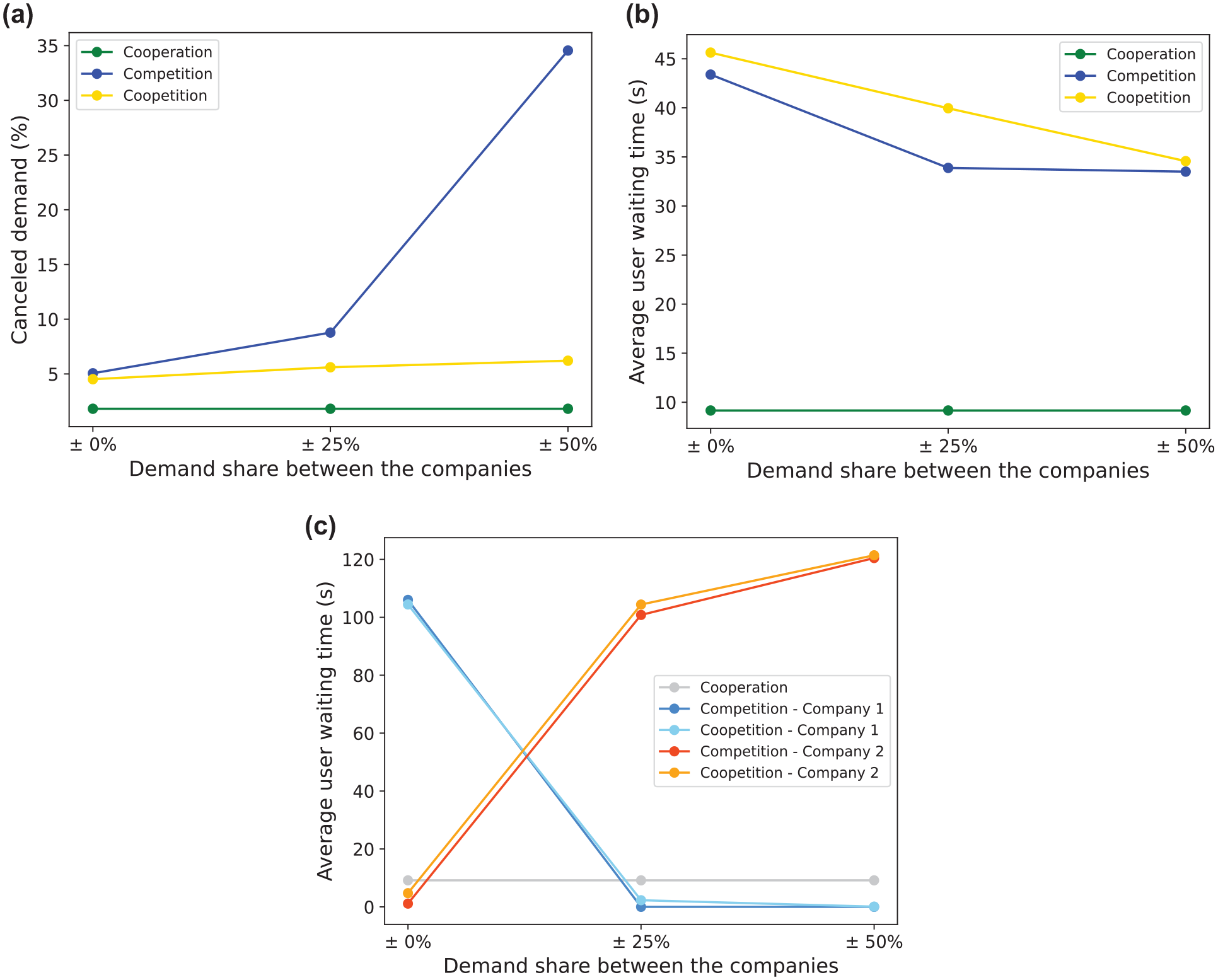
Different demand shares of ride-hailing companies: (a) percentage of canceled demand, (b) average passenger waiting time to be matched, and (c) average passenger waiting time to be matched by company.

As can be seen from Figure 12c, the approximate fair demand share between the two companies would be an additional +12.5% to the demand of Company 1 and −12.5% for Company 2 compared with the benchmark demand level. We can see that even though Company 2 has a bigger fleet, the increase in demand, which is beyond the company’s service capabilities, influences drastically its passengers’ waiting time (Figure 12c), which leads to increased demand cancelation (Figure 12a). This, in return, decreases the vehicle utilization rate of Company2 and lowers the quality of service. The changes in the average user waiting time shown in Figure 12b can be explained by the more detailed Figure 12c. It is noteworthy that, the same as in the fleet share experiment, the changes in the demand share influence more drastically the outcome of the competition scenario than the coopetition.

System Dynamics for the Reference Scenario

Figures 13 to 15 depict the simulation results for the competition between the two companies over the simulation time horizon represented by the X-axis. The fleet size of Company 1 is 280 vehicles with the following initial distribution: 130 idle non-moving vehicles, 50 idle moving vehicles, and 100 occupied vehicles. The fleet size of Company 2 is 320 vehicles with the following initial distribution: 170 idle non-moving vehicles, 50 idle moving vehicles, and 100 occupied vehicles. We assign more vehicles to one company than to the other. If we split the total number of ride-hailing vehicles between two companies equally, it is equivalent to the situation of pre-optimized fleet size based on demand. This perfectly balanced assignment of vehicles is barely realistic. In fact, companies cannot guarantee to have an optimal fleet to serve their demand. Thus, we try to reproduce the non-optimal allocation of vehicles, that is, when one company has fewer and another has more vehicles to serve the same demand. This allows us to derive extra insights into the competition and cooperation. Both companies have the same demand rate.

Figure 13.

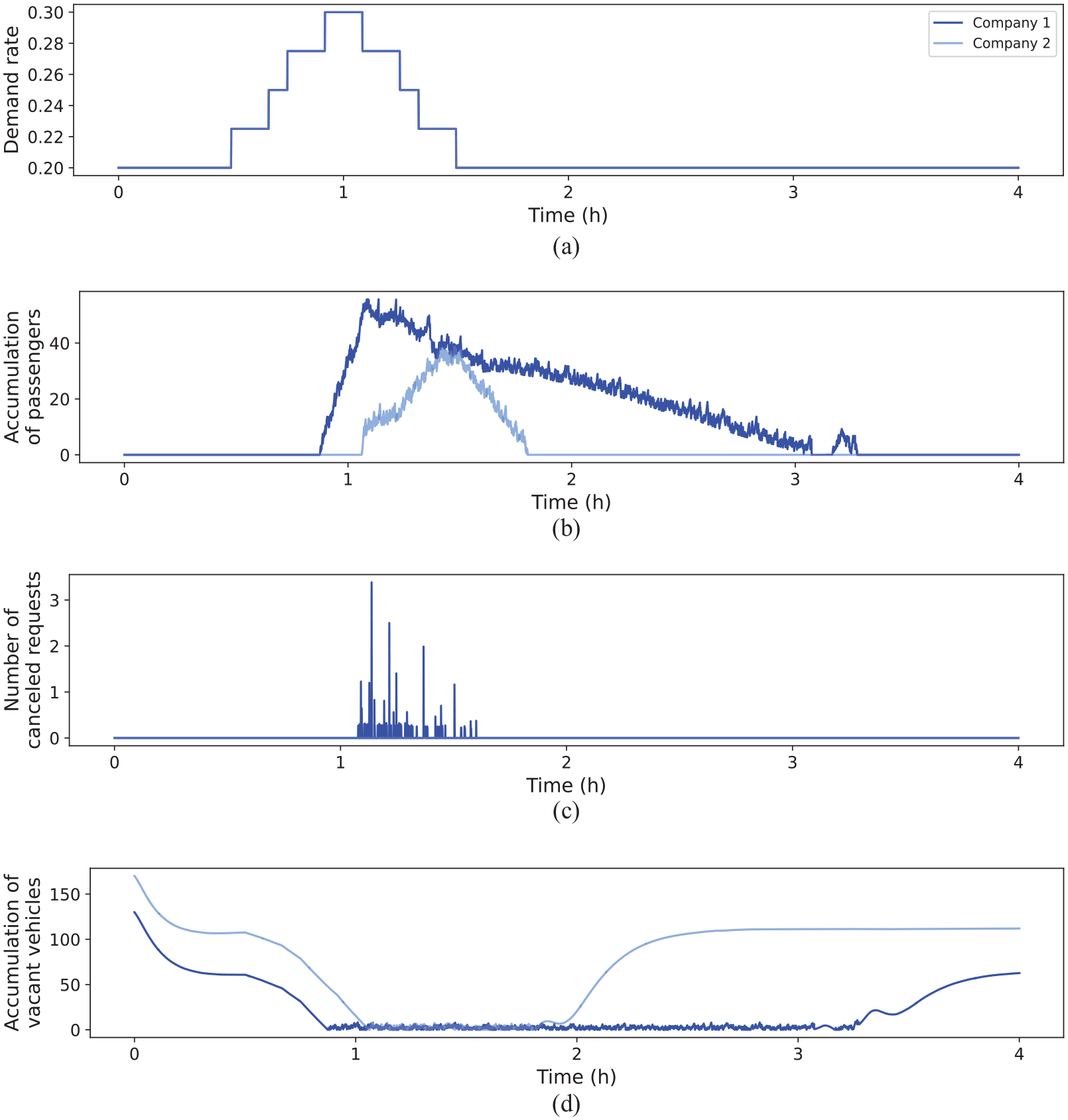
Matching process characteristics: (a) demand rate (the same for both companies), (b) accumulation of waiting passengers to be matched, (c) number of canceled requests, and (d) accumulation of vacant non-moving vehicles.

Figure 14.

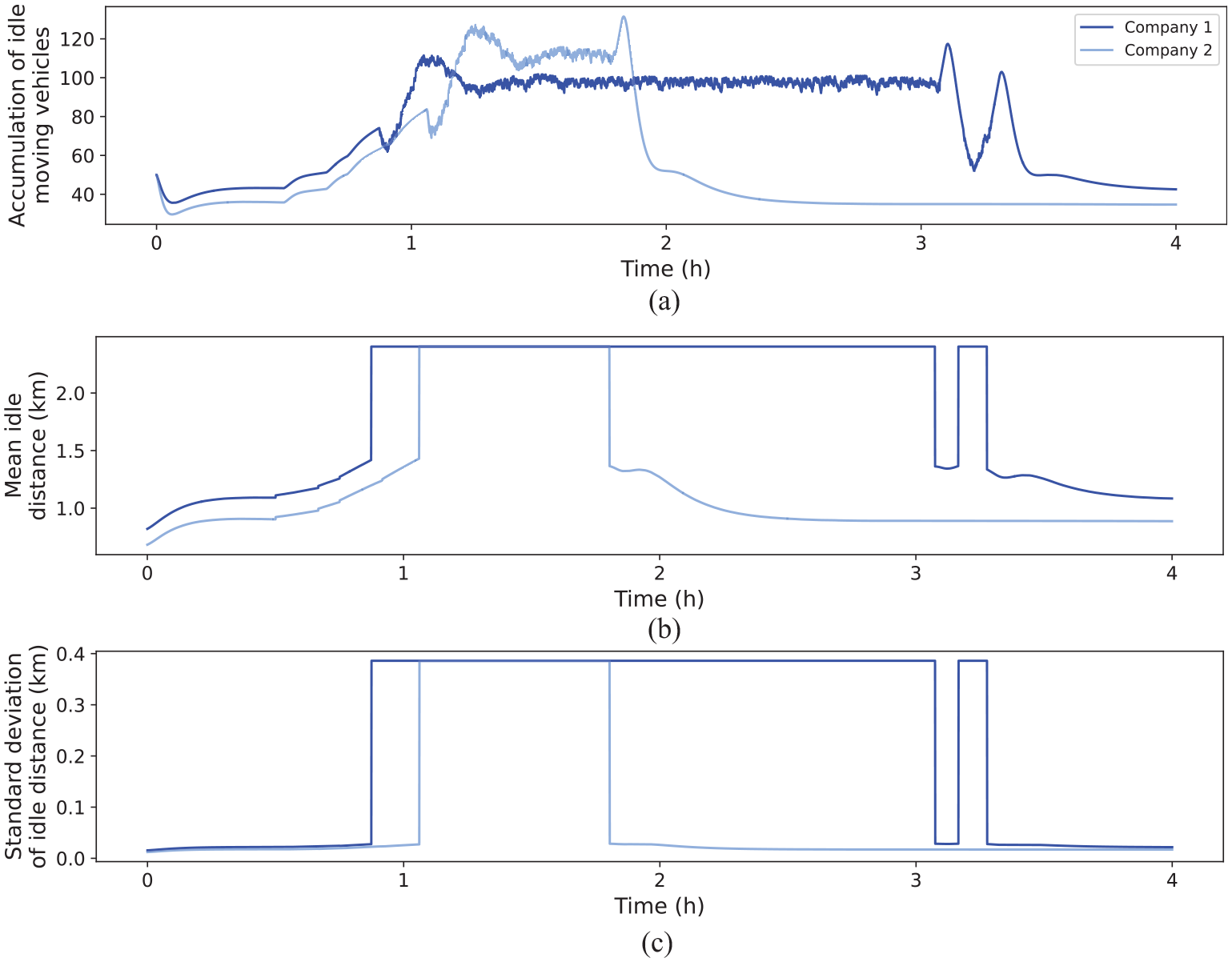
Idle moving vehicles characteristics: (a) accumulation of idle moving vehicles, (b) mean trip length of idle moving vehicles, and (c) mean standard deviation of idle trip length.

Figure 15.

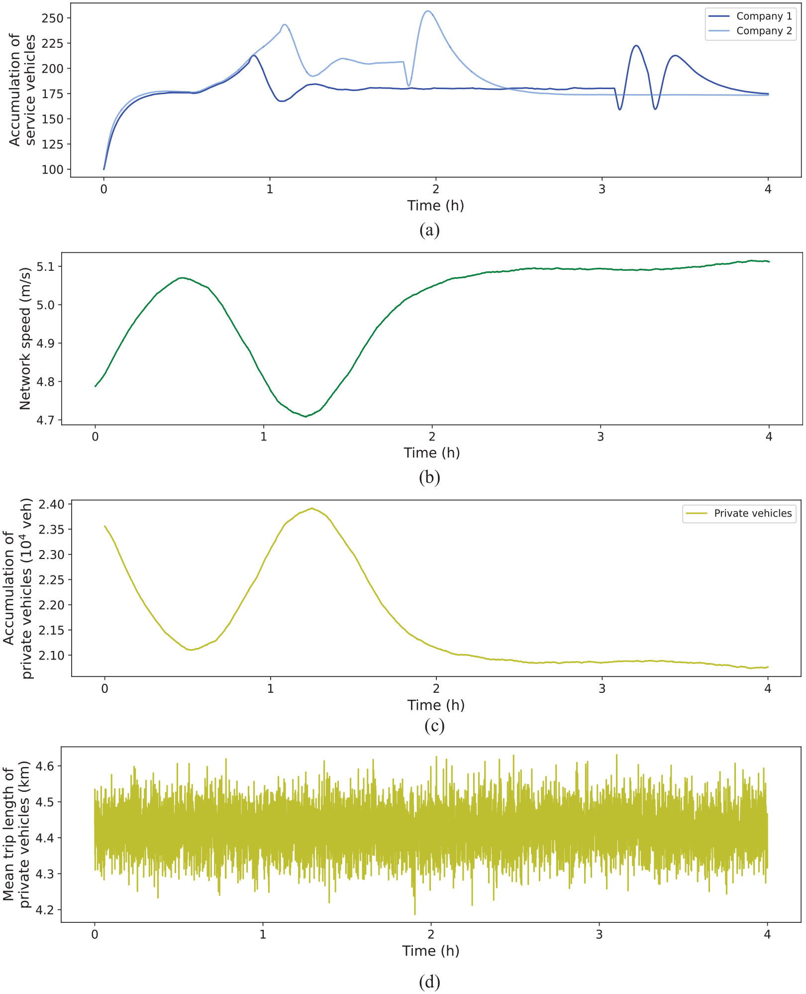
Service vehicles and private vehicles characteristics: (a) accumulation of service vehicles, (b) network speed, (c) accumulation of private vehicles, and (d) mean trip length of private vehicles.

Figure 13 includes the matching process description plots. It contains the evolution graphs of arriving demand requests ${\lambda }^{\mathrm{RH}},$ accumulation of queued non-matched passengers $n^{\mathrm{PAS}},$ number of canceled requests, and accumulation of idle non-moving vehicles $n^I.$ Both companies have the same demand rate, and thus their demand curves overlap. Company 1 runs out of vacant vehicles faster than Company 2 and thus starts accumulating waiting requests earlier. Because of the high accumulation of demand requests in the queue, Company 1 starts canceling them after 3 min waiting time expires. Company 2 runs out of vacant vehicles approximately 500 s (∼8.3 min) later than Company 1 and starts accumulating waiting demand requests. However, none of the waiting requests of Company 2 reach the 3 min waiting time limit, and so there are no cancelations for Company 2.

Figure 14 shows the plots describing the evolution of the idle moving vehicles component. It includes the accumulation of the idle moving vehicles $n^{\mathrm{RHI}},$ their mean idle trip length $L^{\mathrm{RHI}},$ and mean standard deviation ${\sigma }^{\mathrm{RHI}}$ . We can see the dependence of the accumulation of idle moving vehicles on the mean trip length. We also observe significant changes in average trip length and its standard deviation when a company starts lacking users or having vacant vehicles. Thus, as long as there are users in the queue, the mean idle distance will be 2,403 m. The non-empty queue of customers explains the jumps in the idle distance. In this case, for each match, we draw an idle distance from the distribution and see if it is within the allowed limit. If the idle distance exceeds the maximum matching distance (2,000 m) then the match does not occur. When the queue becomes empty, the idle distance drops to the normal state where it depends on the vacant vehicle density and demand density. It may seem that the standard deviation curve is a step function, but in reality the variation in standard deviations for the non-saturated state is very small (1–15 m) and thus is not visible on the graph compared with the jump in standard deviation for the saturated state (386 m).

Figure 15 depicts both the instance of the service ride-hailing vehicles and private vehicles with the following plots: accumulation of occupied moving vehicles $n^{\mathrm{RH}},$ network speed $v,$ accumulation of private vehicles $n^{\mathrm{PV}},$ and average trip length of private vehicles $L^{\mathrm{PV}}$ (equal to the average trip length of service ride-hailing vehicles $L^{\mathrm{RH}}$ ).

To provide more insights into the evolution of the system-wide metrics according to different scenarios, we compare the evolution of the network speed over time in Figure 16. For the peak hours, when the demand rate is the highest, all scenarios perform similarly in relation to speed. However, when the demand is constant, and the network is not saturated, it is the cooperation scenario that experiences the highest speed, even though it is slightly unstable.

Figure 16.

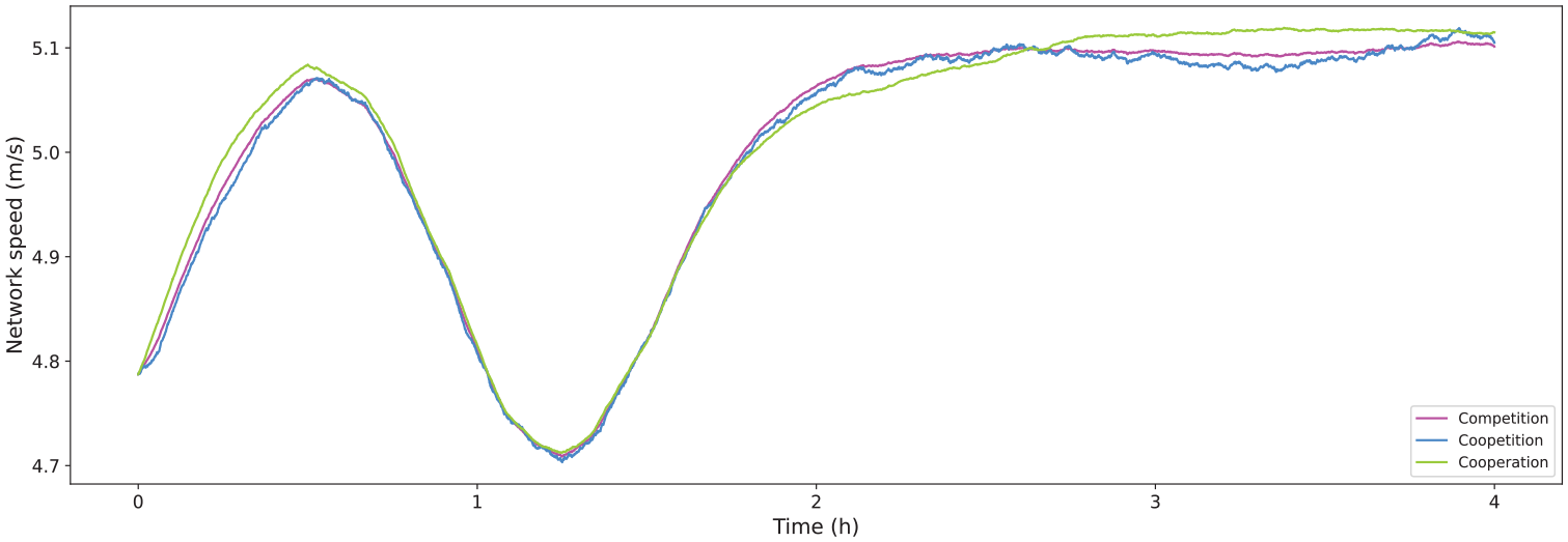
Network speed evolution under different scenarios.

Conclusion

In this work, we address the influence of competition in the ride-hailing market on the system dynamics, congestion level, and service in the short-term perspective. In particular, we investigate how competition influences the passenger–driver matching process, the consequent vehicle travel for picking up the customer, and, more globally, the system at the operational level. To this end, we propose a modeling and simulation framework based on the MFD. We apply the M-model that explicitly monitors the remaining travel distance of all vehicles. In this work, we extend the mathematical M-model decomposition and focus on accurate dynamic estimation of trip lengths for the different vehicle states based on the immediate system state. To do so, we suggest creating an additional proxy modeling framework replicating the demand requests and the service vehicle movements. We propose calibrating the matching function by sampling observations on a grid network of a proxy. By sampling multiple configurations, we study the relation between trip lengths, demand levels, and vacant fleet sizes and calibrate the matching function accordingly. Finally, we assess and compare matching processes that define diverse competition scenarios. Three scenarios are implemented for different initial system settings: competition between companies, cooperation of companies, and competition with partial cooperation (coopetition).

The results show the following tendencies. According to the “System Dynamics for the Reference Scenario” subsection above, the highest speed is experienced in cooperation during off-peak hours, while during peak hours, all scenarios perform similarly in relation to the network speed. Overall, the demand cancelation rate is the highest in the competition scenario, followed by coopetition and cooperation. Generally, the passenger matching waiting time is the longest in the coopetition scenario and decreases in competition and cooperation.

One of the limitations of this paper is the lack of advanced rebalancing strategies. However, as mentioned before, this would require a complete description of the spatial dimension of the problem, which is not possible with the used continuous description of the vehicle states. Still, we would argue that more advanced rebalancing strategies could have a clear impact on waiting time (considering effective rebalancing) but little impact on travel distances.

Note also that there are only two ways to improve the network speed: either because of less total travel distance or because of more trip cancelations. Many cancelations are caused by high matching distance and a shortage of vacant vehicles. We admit that with more advanced rebalancing schemes it would be easier to match the users as the vehicles are better located. However, during the congestion peak in our simulation setting, we observe a lack of supply and the presence of queueing passengers to be matched. The more companies present, the greater the possibility of this situation happening because the available vehicles are less likely to match a passenger’s preferences of company. So, there are not enough vehicles to serve the demand, and thus the distance to cover might be too high (shown by the proxy distribution). This means that there is still a chance that an available vehicle will not be close enough to the customer. In this case, the rebalancing would be redundant as we know exactly where the demand is (waiting passengers), and our matching process defines the required idle travel distance to drive. Thus, we believe that the rebalancing would not be a principal game changer for competition. However, the confirmation is left for further studies. A possible perspective in future is to study how additional authority policies and restrictions or new cooperation scenarios might influence the system and service quality.

Supplemental Material

sj-docx-1-trr-10.1177_03611981231171155 – Supplemental material for Competition in Ride-Hailing Service Operations: Impacts on Travel Distances and Service Performance

Supplemental material, sj-docx-1-trr-10.1177_03611981231171155 for Competition in Ride-Hailing Service Operations: Impacts on Travel Distances and Service Performance by Maryia Hryhoryeva and Ludovic Leclercq in Transportation Research Record