Sage Journals: Discover world-class research

Abstract

Two key aggregated traffic models are the relationship between average network flow and density (known as the network or flow macroscopic fundamental diagram [flow-MFD]) and the relationship between trip completion and density (known as network exit function or the outflow-MFD [o-FMD]). The flow- and o-MFDs have been shown to be related by average network length and average trip distance under steady-state conditions. However, recent studies have demonstrated that these two relationships might have different patterns when traffic conditions are allowed to vary: the flow-MFD exhibits a clockwise hysteresis loop, while the o-MFD exhibits a counter-clockwise loop. One recent study attributes this behavior to the presence of bottlenecks within the network. The present paper demonstrates that this phenomenon may arise even without bottlenecks present and offers an alternative, but more general, explanation for these findings: a vehicle’s entire trip contributes to a network’s average flow, while only its end contributes to the trip completion rate. This lag can also be exaggerated by trips with different lengths, and it can lead to other patterns in the o-MFD such as figure-eight patterns. A simple arterial example is used to demonstrate this explanation and reveal the expected patterns, and they are also identified in real networks using empirical data. Then, simulations of a congestible ring network are used to unveil features that might increase or diminish the differences between the flow- and o-MFDs. Finally, more realistic simulations are used to confirm that these behaviors arise in real networks.

Keywords

operations traffic flow theory and characteristics macroscopic traffic models network

Traffic networks are complex systems made up of numerous moving parts (e.g., vehicles) and infrastructure elements (e.g., links and nodes). Modeling individual vehicle movements or traffic on the numerous component pieces of these systems—and their resulting interactions—is extremely challenging because of the computational complexity involved. Perhaps for this reason, researchers have also studied relationships between traffic flow features aggregated across entire regions or cities for decades ( 1 – 8 ). The earliest studies of this type were descriptive models that could be used to understand how one feature (e.g., vehicle speed or flow) varied with network use. For example, the two-fluid model considered the relationship between average vehicle speed and the fraction of vehicles moving in traffic, and later studies examined how this two-fluid model relationship varied with properties of a network ( 9 , 10 ). One particularly insightful study proposed the existence of a unimodal relationship between average network flow, $q$ (vehicle/lane-time), and average network density, $k$ (vehicle/lane-distance), that—unlike other studies of that era—could be used to describe both uncongested and congested traffic scenarios ( 1 ). However, empirical evidence that confirmed the existence of this relationship in practice—known more commonly as the network macroscopic fundamental diagram (flow-MFD)—only became available much later ( 11 ). This latter study has led to a revival of interest in network-wide traffic flow models and their applications.

One aspect that has been studied in the literature is the conditions under which flow-MFDs might arise in practice. One seminal study found that traffic networks should have either uniform or repeatable congestion distribution patterns for well-defined flow-MFDs to arise ( 12 ). However, several studies have found that traffic networks have a natural tendency for congestion to spread unevenly in an unpredictable way, which can result in highly scattered or poorly defined flow-MFDs ( 13 – 15 ). This unstable behavior also leads to hysteresis patterns in which flows are lower when congestion dissipates than as it grows in a network, and this behavior manifests as clockwise loops on the flow-MFD ( 16 – 18 ). These natural tendencies toward unpredictable inhomogeneous congestion distributions can be somewhat mitigated by providing vehicles with advanced information to avoid already-congested areas within a network or utilizing adaptive traffic signal control to prioritize movement away from more-congested areas ( 16 , 18 –20). Traffic networks can also be carefully partitioned into smaller regions with more uniform congestion patterns to yield more well-defined flow-MFDs ( 21 – 24 ).

While flow-MFDs are generally descriptive (i.e., used to describe how well a network might be operating or compare operations across certain conditions), aggregated relationships such as MFDs can also be used to describe traffic network dynamics on a regional level. One study showed how the existence of a flow-MFD also implies the existence of a relationship between the rate at which trips can be completed in a network, $f$ (trips/time), and its use (measured either by average density or average number of vehicles circulating within the network, $n$ [vehicles]) ( 25 ). This latter relationship has sometimes been called the network exit function of outflow macroscopic fundamental diagram (o-MFD). Various studies have used o-MFD-based modeling frameworks to develop regional traffic control strategies such as perimeter metering control, physics-based regional congestion pricing street network design, and regional routing schemes, among others.

Under steady-state conditions, the flow- and o-MFDs are related in the following way:

f = \frac{q \times L}{l}

(1a)

n = k \times L

(1b)

where

$L$ = lane-distance (the total length of streets in the network), and

$l$ = distance/trip (the average trip length in the network) ( 25 ).

Given the relationships in (1), one would expect that the shape and pattern of the flow- and o-MFD would be similar. For example, if the flow-MFD exhibits clockwise hysteresis loop patterns, then the o-MFD should exhibit a similar shape. However, this does not turn out to be the case. Recent studies used different traffic flow models (e.g., Lighthill-Whitham-Richards (LWR), accumulation-based, and trip-based) to investigate traffic network dynamics under fast-varying demand conditions and found that the o-MFD may exhibit counter-clockwise hysteresis patterns even while the flow-MFD exhibits no hysteresis pattern or clockwise hysteresis patterns ( 26 – 29 ). One study attributed this pattern to the presence of internal bottlenecks within the network that cause outflows to sustain their maximum value until all vehicles that experience congestion have left ( 28 ).

In this present study, we first examine the shapes and patterns of the observed flow- and o-MFDs under fast-varying demand conditions (thus in an unsteady state) on an arterial case where no bottleneck is present to demonstrate that the conflicting hysteresis patterns are not necessarily caused by the presence of internal bottlenecks. Instead, we demonstrate that these are caused by differences in how the flow- and o-MFD are computed: the former considers the entire length of a vehicle’s trip, while the latter only considers its end. Then, we show and explained that, when the trip distance heterogeneity is significant, there could be both clockwise and counter-clockwise hysteresis loops and thus a figure-eight pattern in a network’s o-MFD, even with no or opposite loops in the flow-MFD. This is followed by empirical evidence demonstrating that these findings also hold in real-world MFDs. Finally, we use a simple network simulation to verify the existence of counter-clockwise and figure-eight hysteresis patterns in the o-MFD and examine how various features might influence the size and shape of these conflicting hysteresis patterns.

The remainder of this paper is organized as follows. First, a simple corridor example is studied analytically to unveil the contradictory patterns between the flow- and o-MFDs under fast-varying demand. Analytical explanations are provided for the existence and cause of the counter-clockwise hysteresis loop and figure-eight patterns in the o-MFD in the absence of bottlenecks even without hysteresis in the flow-MFD. The presence of such patterns is also demonstrated using empirical data. This is followed by the investigation of the impact of different network features on the magnitude of the hysteresis loop in the o-MFD using microscopic simulations. Finally, some discussion and concluding remarks are offered.

Cause of Counter-Clockwise Hysteresis Patterns in the O-MFD

One most recent explanation for the counter-clockwise loop in the o-MFD is provided in Leclercq and Paipuri, which investigated the behavior of traffic states on a long arterial and attributed the counter-clockwise loop to the presence of an internal bottleneck ( 28 ). In this section, a simple arterial that has no bottlenecks is first analyzed to show that counter-clockwise pattern may still arise in the o-MFD when no internal bottlenecks are present. This loop exists even when the flow-MFD exhibits no loop. In addition, an arterial with two exits and a two-bin system are also analyzed to demonstrate that other patterns might exist—for example, simultaneous clockwise and counter-clockwise hysteresis loops in the o-MFD (thus a figure-eight pattern). Note, we specifically focus on observed relationships in this paper and use the terms flow-MFD and o-MFD to refer to these observed relationships, as opposed to steady-state relationships that would occur under time-invariant demands.

Measurement Lag

In this section, traffic behavior on a long arterial will be used to demonstrate why a counter-clockwise hysteresis loop can be observed in the o-MFD when demand varies quickly.

Scenario Setup

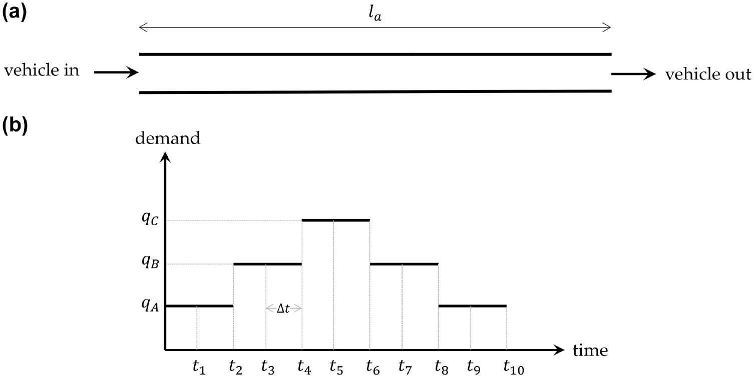
We consider here a one-way arterial of length $l_{a}$ (length) with a single entrance and exit (see Figure 1a). This arterial is assumed to have a single travel lane and, more critically, contain no internal bottlenecks. Traffic on the arterial is assumed to obey a triangular fundamental diagram with a common free-flow speed $v_{f}$ (length/time), capacity $Q_{m}$ (vehicle/time), and jam density $k_{j}$ (vehicle/length). As shown in Figure 1a, vehicles enter the arterial from the left side and travel toward the right. Vehicles are assumed to exit without any external disruptions—that is, there are no external restrictions to vehicle exit rate.

Figure 1.

(a) Illustration of one-way arterial setup and (b) demand profile used for analytical investigation.

Vehicles are assumed to enter an initially empty arterial following the demand profile shown in Figure 1b. The demand pattern mimics a typical rush with a loading period (from time 0 to $t_{4}$ [time]) in which demand increases from 0 to its maximum value of $q_{C} < Q_{m}$ , the peak in which the maximum demand $q_{C}$ is maintained (from time $t_{4}$ to $t_{6}$ ), and then a recovery period in which the demand drops from $q_{C}$ to 0 (from time $t_{6}$ to $t_{10}$ ). To simplify the analytical investigation and without lack of generality, the loading period and recovery period are assumed to consist of periods that have constant intermediate demands $q_{A} < q_{B} < q_{C}$ . Furthermore, we assume that each period of constant demand is maintained for a period of $2 Δ t$ , where $Δ t$ is the time for a vehicle to completely traverse the arterial at the free-flow speed. Thus, the entire rush occurs over a period of $10 Δ t$ . These latter two assumptions are not necessary and will be relaxed so that demand is allowed to vary throughout the loading and recovery period in the simulation verification.

Analytical Analysis of Flow-MFD and o-MFD Shape

Traffic dynamics on this simple arterial can be readily described using the theory of kinematic waves proposed by Lighthill and Whitham, and Richards ( 30 – 32 ). Figure 2a provides a time-space diagram that describes how traffic states evolve along the arterial given the conditions considered. Solid black lines represent interfaces that separate unique traffic states—indicated by colored regions in the figure denoted O, A, B, and C—that arise along the arterial. 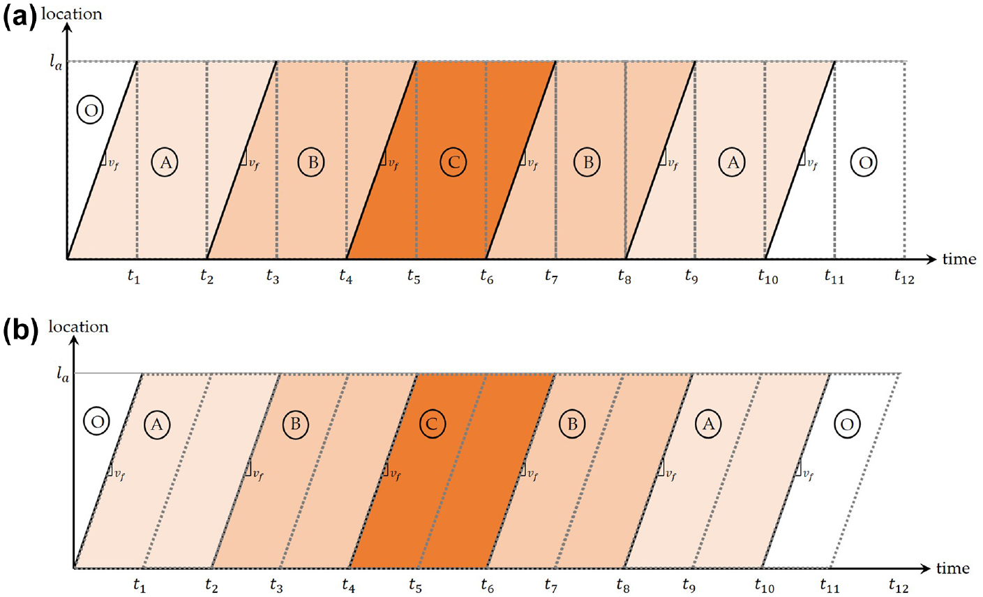Note that O refers to the zero state in which density and flow are zero, whereas any other state $i$ refers to the associated free-flow state with flow $q_{i}$ . All interfaces move along the time-space plane at the free-flow speed, since congestion does not arise along the arterial because of the lack of bottlenecks or external restrictions.

Figure 2.

Time-space diagram describing traffic dynamics on arterial under given demand conditions: (a) traditional measurement intervals and (b) skewed measurement intervals.

We first consider the shape and pattern of the flow-MFD. Again, for simplicity of calculation and without lack of generalization, let us assume that flow and density are aggregated at regular time intervals of $Δ t$ (denoted by the dashed gray rectangles in Figure 2). Based on the generalized definitions of Edie, the average flow (likewise density) during any measurement interval is computed as the area-weighted average of the flow (density) in each observed traffic state within that interval ( 34 ). For example, the average flow during the first measurement interval from time 0 to $t_{1}$ is $\frac{1}{2} (q_{0} + q_{A}) = \frac{1}{2} q_{A}$ . The resulting flow-density relationship obtained from the time-space diagram in Figure 2a is shown on the left side of Figure 3a. As expected, all observed flow-density points lie along the free-flow branch of the fundamental diagram since all observed traffic states are in free flow. More importantly, no hysteresis patterns are observed in the flow MFD.

Figure 3.

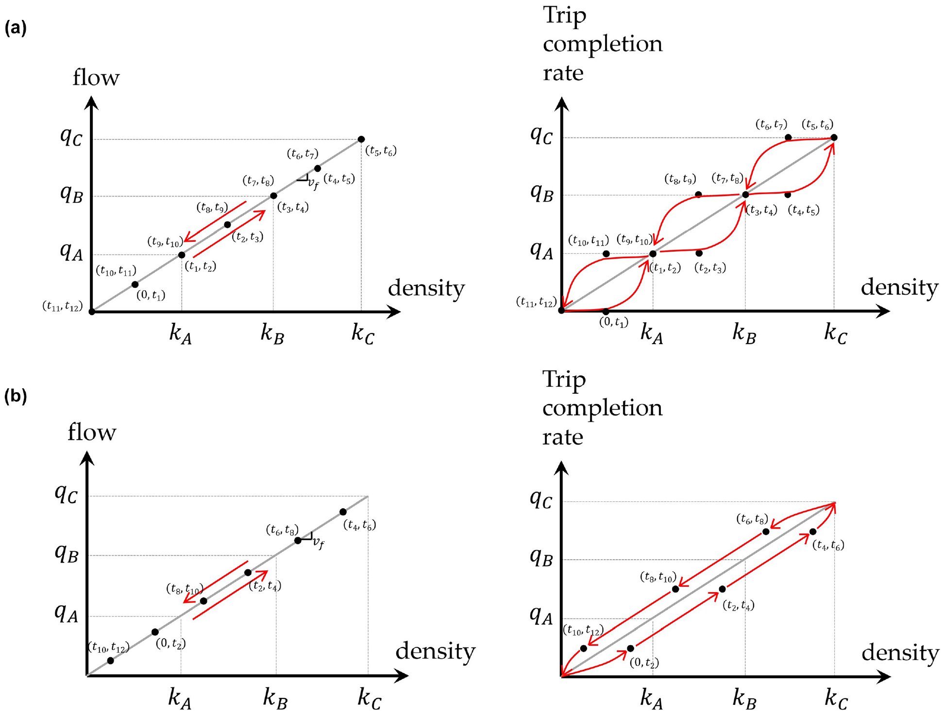
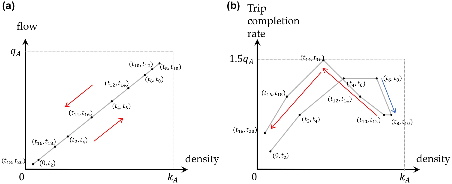
Flow macroscopic fundamental diagram (flow-MFD) and outflow macroscopic fundamental diagram (o-MFD) for the simple arterial example under: (a) constant demand periods of length $2 Δ t$ and (b) constant demand periods of length $Δ t$ .

Next, we consider the shape and pattern of the o-MFD. As average accumulation and density are equivalent to a multiplicative constant (arterial length, $l_{A}$ ), we consider the relationship between trip completion rate and density as the o-MFD here. The trip completion rate is simply the rate of trips that leave the arterial section and can be calculated as the flow measured at the end of the arterial (horizontal line at location $l_{A}$ in Figure 2). The resulting o-MFD is provided on the right side of Figure 3a. Notice that the o-MFD generally exhibits a counter-clockwise hysteresis pattern in which trip completion rates are lower as density along the arterial increases (i.e., during loading) than as it decreases (i.e., during recovery). This occurs even without the presence of bottlenecks along the arterial for a simple reason: average flow during a measurement interval is computed based on overall vehicle movements during that measurement interval, whereas trip completion rate is only influenced by vehicle movement at the end of the arterial. For example, the flow is positive during the first measurement interval since vehicles have entered and are traveling along the arterial. However, the trip completion rate is zero since no vehicles have reached the end of the arterial to exit the system. Put another way, average flow is a measurement of overall movement along the arterial, while trip completion rate is only a measurement of vehicles reaching the end of their trip. Thus, in the context of this example, trip completion rate “lags” after average flow: changes in entering demand are immediately incorporated into the calculation of average flow, whereas they only influence trip completion rate after some time $Δ t$ , in which the first vehicle in the new traffic state arrives at the downstream end of the arterial. If trips could start and end within the same measurement interval, the hysteresis would entirely disappear. For example, consider if the flow-MFD and o-MFD were computed using the skewed measurement intervals in Figure 2b which are similar to intervals for flow measurements in Laval ( 33 ). Here, each measurement interval is the same size in the time-space plane as those in Figure 2a, but is skewed so they move forward in space at the free-flow speed. In this case, a single traffic state would be observed during the entire measurement interval; thus, the flow-MFD would be the same as the free-flow branch of the fundamental diagram, and the o-MFD would exhibit no hysteresis. However, while useful in this arterial context, such skewed measurement intervals are not feasible for network-wide operations since trips start and end throughout the network and, thus, the hysteresis patterns are bound to arise when traditional measurement intervals are used.

Note also that the trip completion rate is the same at some density values ( $k_{A}, k_{B}, k_{C}$ ) during loading and recovery in Figure 3a. This occurs because of the specific stepwise demand pattern considered used for simplicity of calculations. Long periods of constant demand allow the network to return to a steady-state condition in which the flow-MFD and o-MFD are consistent. If demand is more variable over time (i.e., the same demand does not persist for as long), more clear hysteresis patterns emerge. As an example, Figure 3b provides the flow- and o-MFDs for the case where the length of each constant demand period reduces from $2 Δ t$ to $Δ t$ . The change has no impact on the flow-MFD but results in a much clearer counter-clockwise hysteresis pattern in the o-MFD.

Trip Distance Heterogeneity

In the previous section, we studied the o-MFD of a simple arterial with one entrance and one exit (thus the same trip distance) under a fast-varying demand pattern and found that the measurement lag between trip completion rate and average flow/density led to a counter-clockwise hysteresis loop in the o-MFD. In this section, a simple arterial with multiple exits (resulting in different trip distances) is studied. As will be shown here, the trip distance heterogeneity causes a lag of outflows at different exits leading to a figure-eight pattern in the o-MFD.

Scenario Setup

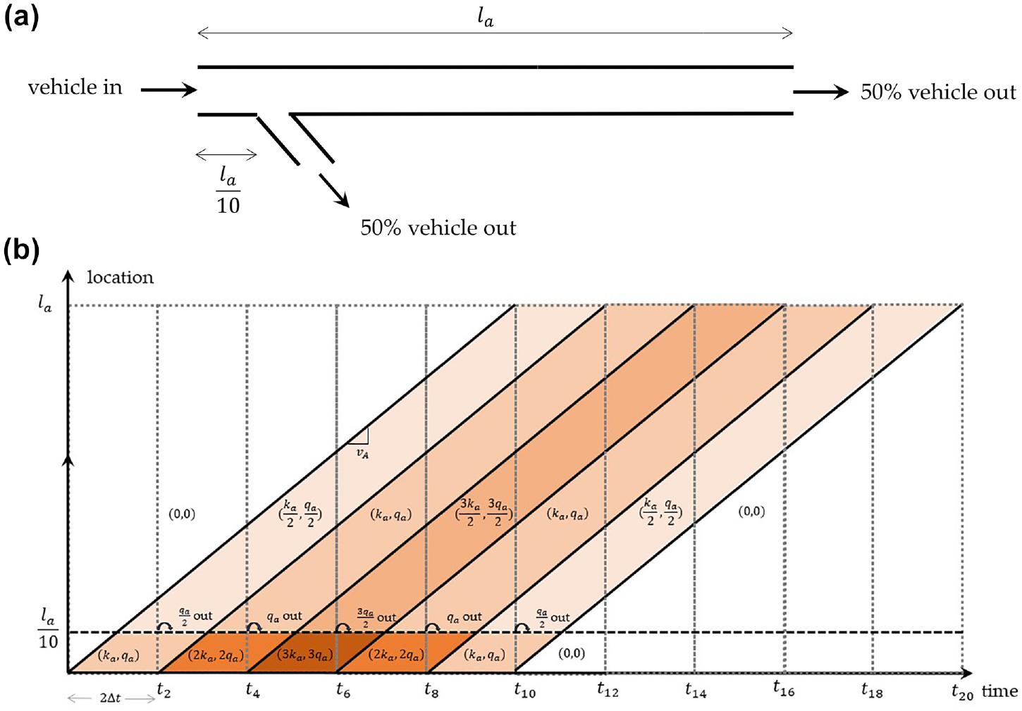
We consider the same arterial as in the previous section, except that there is another exit located $l_{a} / 10$ away from the entrance, shown in Figure 4a. It is assumed that half of the vehicles entering the arterial will leave at the first exit and half of the inflow will leave at the last exit.

Figure 4.

(a) Illustration of one-way arterial with two exits and (b) time-space diagram describing traffic dynamics on an arterial with two exits.

Vehicles are assumed to enter an initially empty arterial following the same demand profile shown in Figure 1b. For simplicity, we assume $q_{A} < q_{B} = 2 q_{A} < q_{C} = 3 q_{A}$ . Each period of constant demand is maintained for a period of $2 Δ t$ , where $Δ t$ is the travel time from the entrance to the former exit at the free-flow speed. Thus, the travel time from the entrance to the latter exit at the free-flow speed is $10 Δ t$ .

Analytical Analysis of Flow-MFD and o-MFD Shape

Similarly, traffic dynamics on this simple arterial can be described using the theory of kinematic waves. Figure 4b provides a time-space diagram that describes how traffic states evolve along the arterial given the conditions considered. Solid black lines represent interfaces that separate unique traffic states with flow and density as a function of $k_{a}$ and $q_{a}$ arising along the arterial.

Let us assume that flow and density are aggregated at regular time intervals of $2 Δ t$ . Based on the generalized definitions, the calculated flow-density relationship is shown in Figure 5a ( 34 ). Similar to the MFD of a simple arterial with one exit, all observed flow-density points lie along the free-flow branch of the fundamental diagram and no hysteresis pattern is observed. The resulting o-MFD is then provided in Figure 5b. Interestingly, we can observe a combination of both clockwise and counter-clockwise loops exhibiting a figure-eight pattern—that is, the trip completion rate is higher during loading than during recovery for a higher density, and lower during loading than during recovery for a lower density. This occurs simply because the difference in trip distance of different vehicles leads to a lag of trip completion rates between the two exits. Specifically, after 50% of vehicles from the loading and peak period leave the arterial at the first exit, the other 50% of vehicles from the loading and peak period have not yet reached the last exit. As a result, the trip completion rate drops as the inflow drops, corresponding to the blue trajectory in Figure 5b. As shown in Figure 4b, when the other 50% of vehicles from loading and peak period start to leave at the last exit at $t_{10},$ no more vehicles leave at the first exit, while trip completion rate at the last exit follows a similar pattern as the inflow—that is, it increases first, remains at a constant value, and finally decreases. This corresponds to the red trajectory in Figure 5b. These two trajectories form a clockwise hysteresis loop at a higher density and a counter-clockwise hysteresis loop at a lower density, exhibiting a figure-eight pattern. This figure-eight pattern should be generally expected in freeway o-MFDs as the exits of freeways are far away from each other leading to a significant lag of trip completion rate between different exits.

Figure 5.

(a) Flow macroscopic fundamental diagram (flow-MFD) for an arterial with two exits and (b) outflow macroscopic fundamental diagram (o-MFD) for an arterial with two exits.

Empirical Evidence

In this section, empirical evidence of hysteresis patterns in the o-MFD is provided. First, evidence of this counter-clockwise hysteresis behavior in the o-MFD is found for an urban network in Shenzhen, China. Second, similar evidence is identified for a freeway in the Netherlands in the existing literature. These results reveal that the patterns unveiled in the simulation also exist in real data.

Shenzhen Nanshan District

Evidence for the existence of a figure-eight pattern in a network’s o-MFD is first obtained from empirical data in Shenzhen, China. The dataset used for that study is a large-scale vehicle location dataset captured by the App called Baidu Map (https://map.baidu.com/). Data of Nanshan district in the dataset are analyzed in this paper because a higher demand is observed in this district during the peak hour.

In Figure 6a, we can observe a small counter-clockwise hysteresis loop at a medium density formed by the loading period (6:00–9:00) and recovery period (9:00–12:00), and a large clockwise hysteresis loop at a higher density formed by the loading period (15:00–18:00) and recovery period (18:00–21:00). In Figure 6b, we can observe a large counter-clockwise hysteresis loop at a medium density formed by the loading period (6:00–9:00) and recovery period (9:00–12:00), and a small clockwise hysteresis loop at a higher density formed by the loading period (9:00–12:00) and recovery period (12:00–15:00). These prove the existence of a figure-eight pattern in the o-MFD in real-life urban networks.

Figure 6.

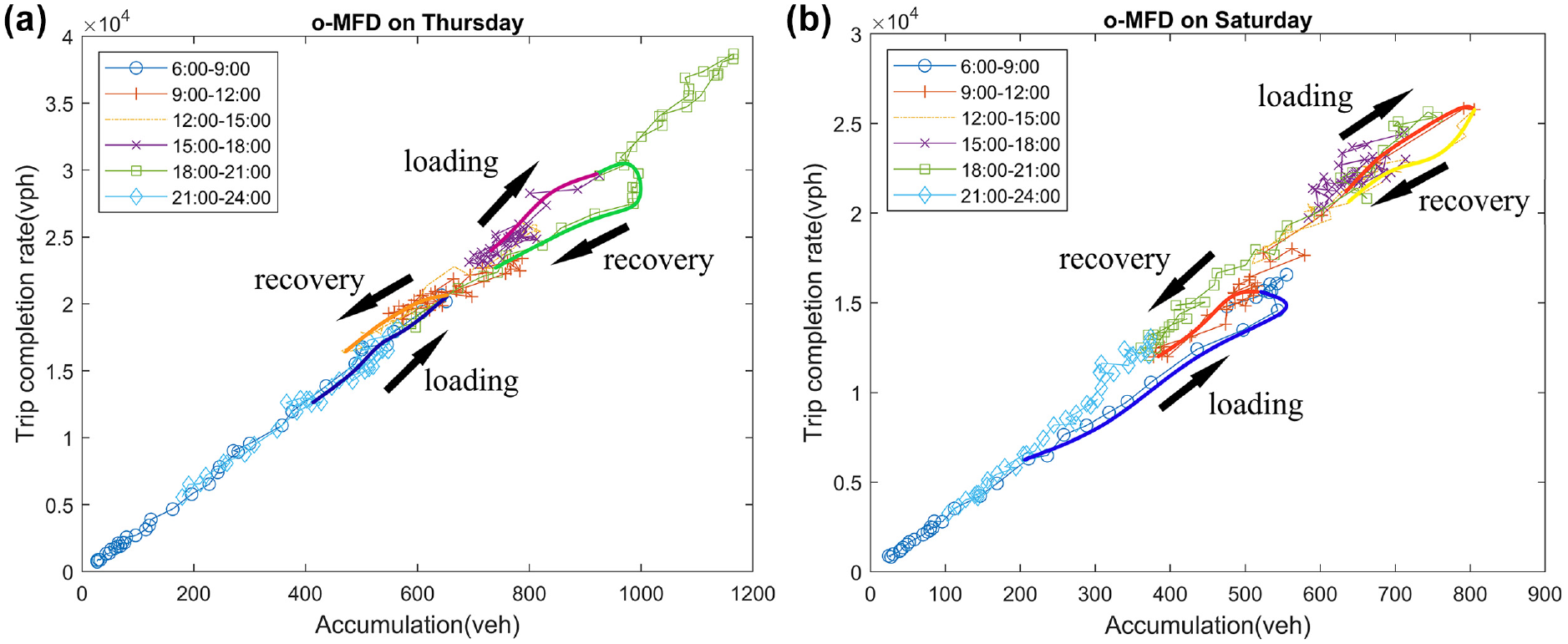
Outflow macroscopic fundamental diagram (o-MFD) in Nanshan district on: (a) Thursday and (b) Saturday.

Dutch Freeway

Furthermore, there is also empirical evidence to support the finding of figure-eight patterns in the o-MFD from existing literature. One example is provided in Figure 7, which shows the flow-MFD and o-MFD of Dutch freeway A13-L ( 35 ). The freeway stretch is about 16 km in length and includes six on-ramps and six off-ramps.

Figure 7.

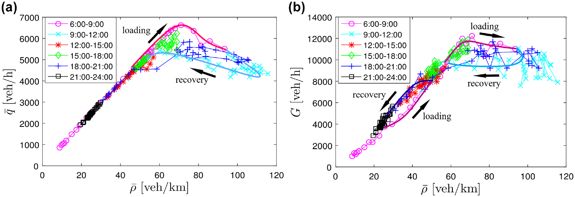
Example of empirical evidence from Han et al.: (a) flow macroscopic fundamental diagram (flow-MFD) and (b) outflow macroscopic fundamental diagram (o-MFD) ( 35 ).

In the flow-MFD in Figure 7a, we can clearly observe no hysteresis loop in the free-flow regime and a clockwise hysteresis loop in the capacity regime formed by the loading period (6:00–9:00) and recovery period (9:00–12:00). By contrast, o-MFD in Figure 7b has a figure-eight pattern—that is, a counter-clockwise hysteresis loop can be seen in the free-flow regime formed by the loading period (6:00–9:00) and recovery period (21:00–24:00), while a clockwise hysteresis loop can be observed in the capacity regime formed by the loading period (6:00–9:00) and recovery period (9:00–12:00). This validates the existence of a figure-eight pattern in the o-MFD caused by lag of trip completion because of the trip distance heterogeneity.

Potential Treatment for the Impact of Lags

In the previous sections, we studied the causes of the hysteresis patterns in the o-MFD under a fast-varying demand pattern and found that the measurement lag and lag because of trip distance heterogeneity may lead to a counter-clockwise or a figure-eight hysteresis loop in the o-MFD. It is also found that the shape of the o-MFD under fast-varying demand is not in line with the shape of the flow-MFD and, thus, is not reliable. In this section, we provide potential treatments that could avoid or mitigate the impact of these lags on the o-MFDs so that the o-MFDs are more consistent with the flow-MFD.

The first way to avoid the impact of the lags on the o-MFD is transforming flow-MFD into o-MFD, as per Equation 1. This requires knowledge of both the total length of streets in the network $L$ (lane-distance) and the average trip length in the network $l$ (distance/trip). Because of the linear relationship between network flow and trip completion rate, the resulting o-MFD (named “analytical o-MFD” in the rest of the paper) should share the same shape as the flow-MFD and, thus, is not affected by the lags.

The second method introduces a lag into the measurement of trip completion rate. In the previous section(s), we have shown that the hysteresis pattern in the o-MFD is caused by a mismatch of average network density and trip completion rate. It is also shown that, if a skewed measurement interval is used, the o-MFD will not be affected by the measurement lag and will have the same shape as the flow-MFD. However, the calculation for the average density of such skewed measurement intervals is not feasible in real networks. Thus, the trip completion associated with a given time interval used to measure average density (or accumulation) can be associated with a time interval of the same length but shifted forward in time by some amount. Since the goal is to measure trips that contributed to the measurement of density/accumulation, the average trip travel time is proposed as the amount of shift. This can be dynamically estimated based on measured travel times within the network. We will denote this as the “shifted o-MFD” in the remainder of this paper.

Impact of Network Features on the Hysteresis Patterns

In the previous section, we analyzed the causes of hysteresis patterns in the o-MFD of a few simple networks under fast-varying demand. In this section, we examine the behavior of a ring network and a grid network via microscopic simulations to demonstrate the existence of counter-clockwise patterns and figure-eight patterns in more realistic networks because of the same reasons outlined in the previous section if measured in the traditional way, and how the proposed solutions would affect the measured o-MFDs. We also examine how the counter-clockwise hysteresis patterns in the o-MFD may be influenced by various patterns. The demand profile used in all simulations is fast-varying and, thus, the obtained flow-MFDs and o-MFDs are in an unsteady state.

Ring Network

Simulation Setup

The ring network considered here is illustrated in Figure 8a. The ring has a total length of 10 mi and traffic along the ring is assumed to obey a triangular fundamental diagram with the following properties: v_f = 50 mph; Q_m = 2,000 vehicles per hour (vph); k_j = 200 vehicles per mile (vpm). The ring contains four entry/exit ramps that are equally spaced along its length, which serve as origins/destinations (ODs) within the network. Vehicles entering the network are each assigned a specific exit ramp as their destination and will travel along the ring until they reach their assigned destination to exit and are allowed to exit freely. Entry ramps are treated as unsignalized merges in which entering vehicles are assumed to have priority.

Figure 8.

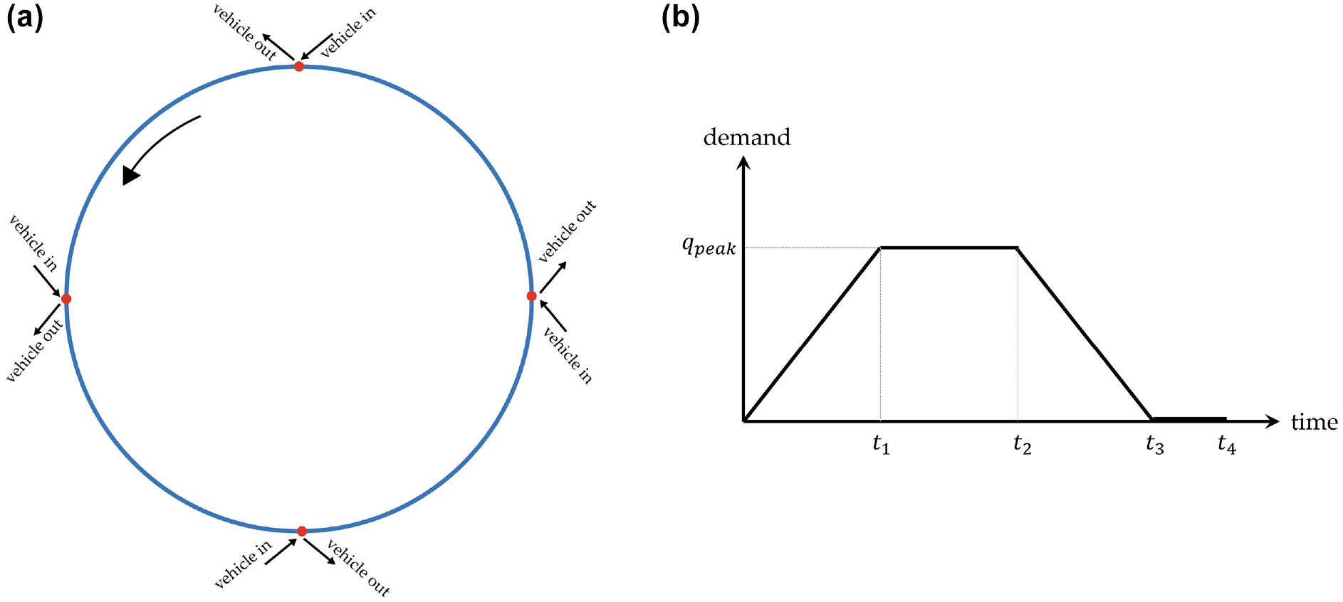
(a) Simulated ring network and (b) demand profile.

The cellular automata model (CAM) consistent with kinematic wave theory is used to simulate the behavior of vehicles on the network ( 36 , 37 ). In this framework, the ring is broken up into homogeneous discrete cells of length 0.005 mi (equal to average vehicle spacing at jam density) that allow only a single vehicle to occupy any cell at any time period. Vehicle locations are updated at consistent intervals of 0.36 s. Average flow and density across the entire network are computed using the generalized definitions of Edie at discrete intervals of 6 min ( 34 ). Trip completion is measured as the rate vehicles exit the ring at their destination exit ramp.

The simulation starts with an empty network. Trips are equally likely to be generated at the four intersections following a specific demand profile (unless otherwise noted). When a vehicle enters the network from an intersection, one of the other three intersections will be assigned to it as the destination based on the trip distance. Different simulations are then conducted to unveil the impacts of different demand and trip distance patterns on the existence and magnitude of the hysteresis loop in the flow-MFD and o-MFD. Vehicles are assumed to enter the ring following the demand profile shown in Figure 8b under the following parameters (unless otherwise specified): t₁ = 1 h, t₂ = 2 h, t₃ = 3 h, t₄ = 3.5 h. In most scenarios, individual vehicle trip distance is set to be 5 mi (i.e., vehicles travel two “segments” and exit at the ramp opposite point of their entry location).

Simulation Results

Peak Demand ( $q_{peak}$ )

The impact of peak demand is first investigated. Figure 9 shows the flow-MFD and o-MFD under peak demand of 2,000, 2,800, and 3,000 vph, respectively. Note that the peak demands represent the total inflow across all four entry ramps; thus, the entry flow at individual ramps has a peak of 500 vph/ramp, 700 vph/ramp, and 750 vph/ramp, respectively.

Figure 9.

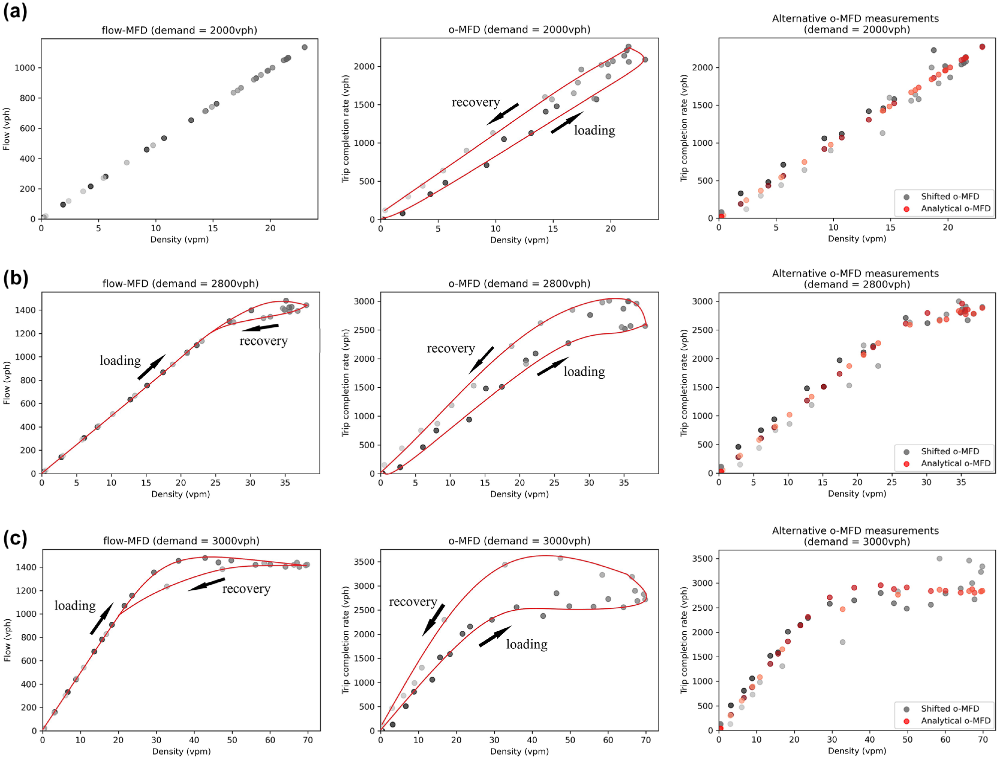
Flow macroscopic fundamental diagram (flow-MFD), outflow macroscopic fundamental diagram (o-MFD), and alternatively measured o-MFD under different peak demands: (a) q_peak = 2,000 vehicles per hour (vph), (b) q_peak = 2,800 vph, and (c) q_peak = 3,000 vph. Darker shades represent measurements performed earlier in time.

The left-hand side of Figure 9 shows the flow-MFDs for the various demand conditions. In the lowest demand case, only the free-flow branch of the flow-MFD is observed and no hysteresis loops arise. In contrast, both the free-flow and congested branches of the flow-MFD are observed under the higher-demand cases. Furthermore, these higher-demand cases exhibit a clear clockwise hysteresis pattern in the flow-MFD as average flows are higher as density increases than as it decreases. This occurs because traffic density along the rings tends toward inhomogeneous spatial distributions as the ring becomes congested ( 13 , 38 ).

The middle column of Figure 9 shows the traditionally measured o-MFD under different peak demands. It can be clearly observed that all three o-MFDs have a counter-clockwise hysteresis loop. This occurs both when the flow-MFD does not have any hysteresis pattern (low demand) and when it exhibits a clockwise hysteresis pattern (higher demands). This demonstrates that the hysteresis pattern in the flow- and o-MFDs can take completely opposite shapes/patterns ( 28 ). However, we show here that this phenomenon occurs even when bottlenecks do not exist within the network. The reason for this, as described in the analytical investigation of a simple arterial in Section 2, is the lagged nature of trip completion rate compared with average flow calculations. Vehicle trips contribute to average flow in the network as soon as they enter the network, but do not contribute to trip completion rate until they reach their destination ramp and exit. Thus, flows increase as demands initially increase as more vehicles arrive onto the network; however, trip completion rate will only increase sometime after, when these vehicles arrive at their destinations. Similarly, even though flow drops as demands decrease when fewer vehicles enter the network, vehicles already in the network still need to arrive at their destination and this would lead to increased trip completion rate even after the demands fall. To demonstrate that the counter-clockwise loop in the o-MFD is caused by measuring the end of vehicles’ trips, Figure 10 plots the average flow in the network for only vehicles within the first and last 25% of their trip, for comparison. That is, flow is computed using the measures of Edie but travel distance only contributes to the flow calculation if the vehicle is within the first 25% (or last 25%) of its travel distance. The results confirm that vehicle flows are higher as density increases for vehicles at the beginning of their trips, but lower as density increases for vehicles at the end of their trips.

Figure 10.

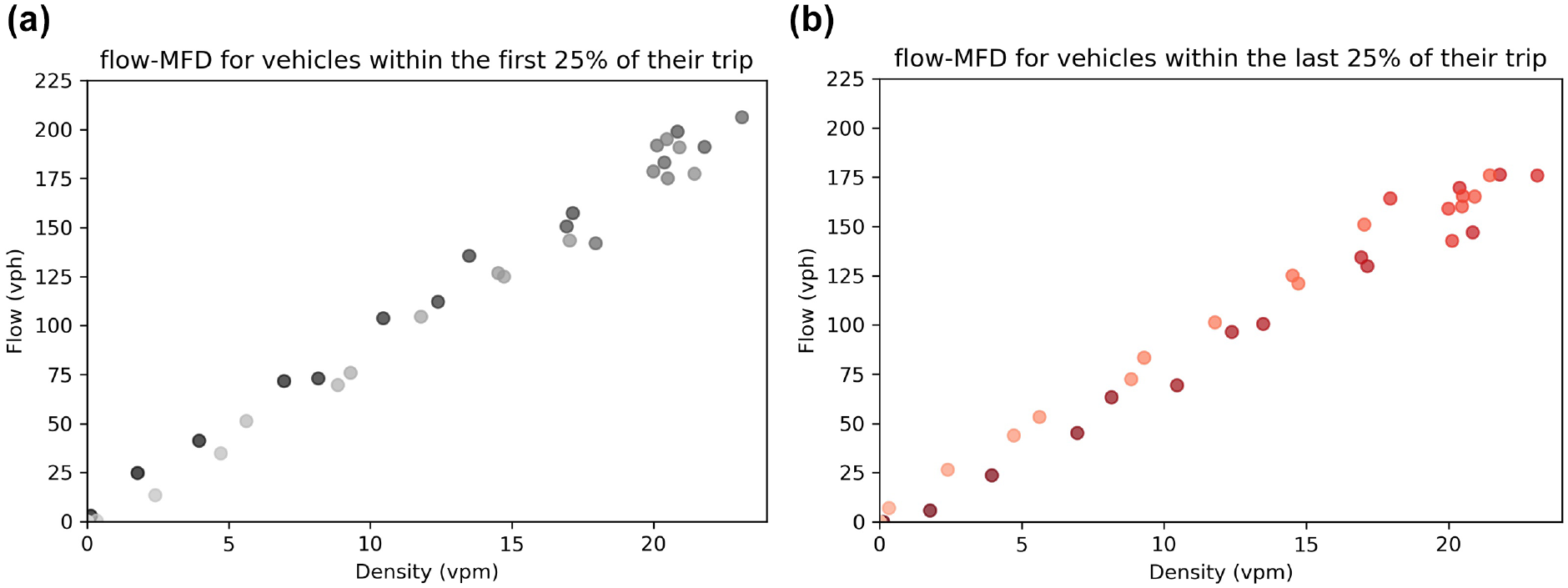
Average flow macroscopic fundamental diagram (flow-MFD) relationship for: (a) vehicles only within the first 25% of their trips and (b) vehicles only within the last 25% of their trips. Darker shades represent measurements performed earlier in time.

Furthermore, comparison of the three o-MFDs in Figure 10 reflects that, as peak demand increases, the size of the counter-clockwise loop in the o-MFD significantly increases because of more vehicles accumulated in the network during the recovery period trying to finish their trips. It is worth mentioning that simulations have also been conducted to investigate the impact of increase in demand change rate during the loading and recovery period on the hysteresis loop in the o-MFD when peak demand is held constant. A similar increase in the size of the loop in o-MFD is observed. This is expected, as more rapidly varying demands will exacerbate the differences between measures of an entire trip (flow) and measures of a trip end (trip completion rate).

Finally, the right-hand side of Figure 9 shows the alternatively measured o-MFDs, either by using the analytical transformation or shifted time measurements. The analytical transformation is simply a rescaling of the flow-MFD and thus shares the same shape. Notice, though, that the counter-clockwise hysteresis loop mostly disappears in the shifted o-MFD that introduces a time lag into the trip completion rate measurement. Instead, a more common clockwise loop is present that matches more closely with the flow-MFD. While not perfect, especially when the network becomes extremely congested, this suggests that using such a shift might provide a more realistic representation of network output as a function of accumulation or density that is in line with the observed flow-MFD.

While not shown (for brevity), similar patterns as the above also emerge as the average trip length increases, since longer trips introduce more congestion in the network (the same as with increased demand).

Demand Distribution

We also examine the impact of demand distribution on the shape of flow-MFD and o-MFD. Figure 11a shows the case where the input demand is evenly distributed across all four intersections—that is, 25% of the total demand enters from each of the four ramps. Figure 11b illustrates the scenario where two opposing ramps each have 30% of total demand entering the network and the other two ramps have 20% of the entering demand each. Similarly, Figure 11c demonstrates the case where two opposing ramps each have 35% of the total input demand and the other two ramps have 15% each. The trip distance in all three cases is set to be 5 mi (two segments), which means vehicles entering at one ramp will leave at the opposite ramp. Therefore, the exiting demand distribution is the same as the input demand distribution in all three cases. The results show that the network will get more congested during the peak hour and thus the size of the loop in both flow-MFD and o-MFD will become larger as demand becomes more unevenly distributed.

Figure 11.

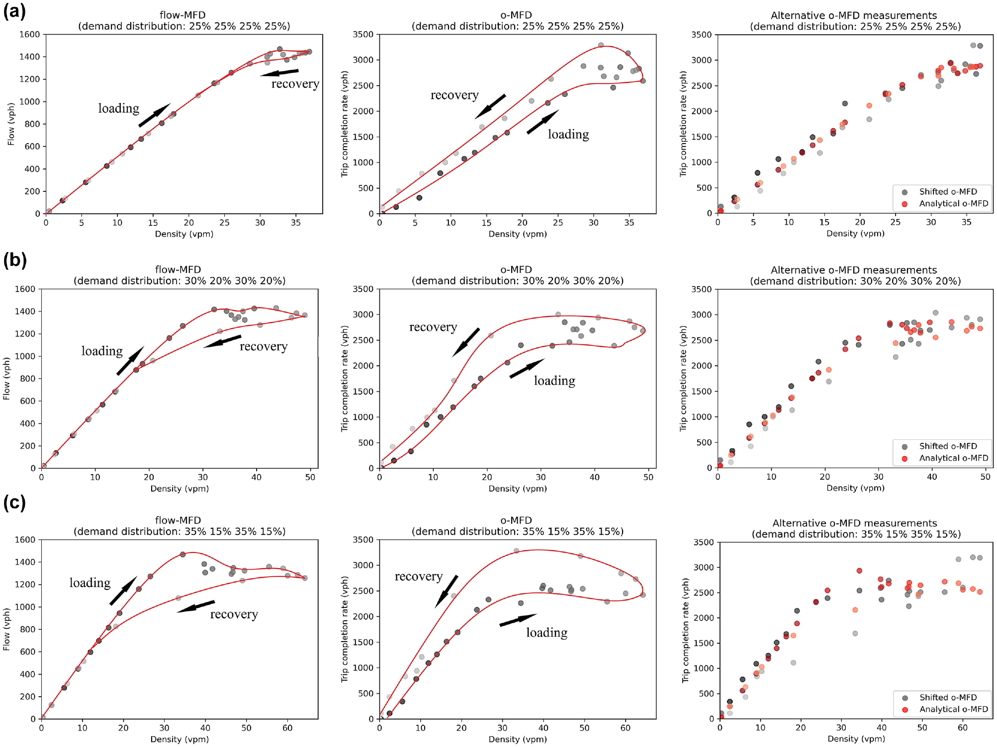
Flow macroscopic fundamental diagram (flow-MFD), outflow macroscopic fundamental diagram (o-MFD), and alternatively measured o-MFD under different demand distribution: (a) total demand evenly distributed at the four ramps, (b) 30%, 20%, 30%, and 20% of total demand distributed at the four ramps, respectively, and (c) 35%, 15%, 35%, and 15% of total demand distributed at the four ramps, respectively. Darker shades represent measurements performed earlier in time.

The alternatively measured o-MFDs are shown on the right-hand side of Figure 11. Similar to the previous section, the shapes of the analytically transformed o-MFDs are much more consistent with the shapes of flow-MFDs than the traditionally measured o-MFDs shown in the middle column of Figure 11, especially for cases when the network is not congested.

Randomness of Trip Distance

Finally, we also consider scenarios in which individual vehicle trip lengths are allowed to vary randomly but maintain a fixed mean value. Figure 12a shows the flow-MFD and o-MFD for the case in which all vehicles travel exactly 5 mi, while Figure 12, b and c , shows the flow-MFD and o-MFD of networks with trip distances ranging from 2.5 mi to 7.5 mi and mean of 5 mi. Clearly, the size of the flow-MFD loop does not change much as trip length becomes more variable. However, the size of the o-MFD loop becomes smaller as trips vary more in length. This is because, when trip distance is not fixed, the fast-completed short trips will quickly contribute to the trip completion during the loading period and will shorten the time that the maximum exit flow rate is maintained during the recovery period. As a result, the exit flow rate will be slightly higher during the loading period and slightly lower during the recovery period compared with the scenario when trip distance is fixed, leading to a smaller size of loop in the o-MFD. Finally, both analytically transformed o-MFDs and shifted o-MFDs on the right-hand side of Figure 12 have similar clockwise hysteresis loops as in the flow-MFDs on the left-hand side of Figure 12 because of the uncongested network.

Figure 12.

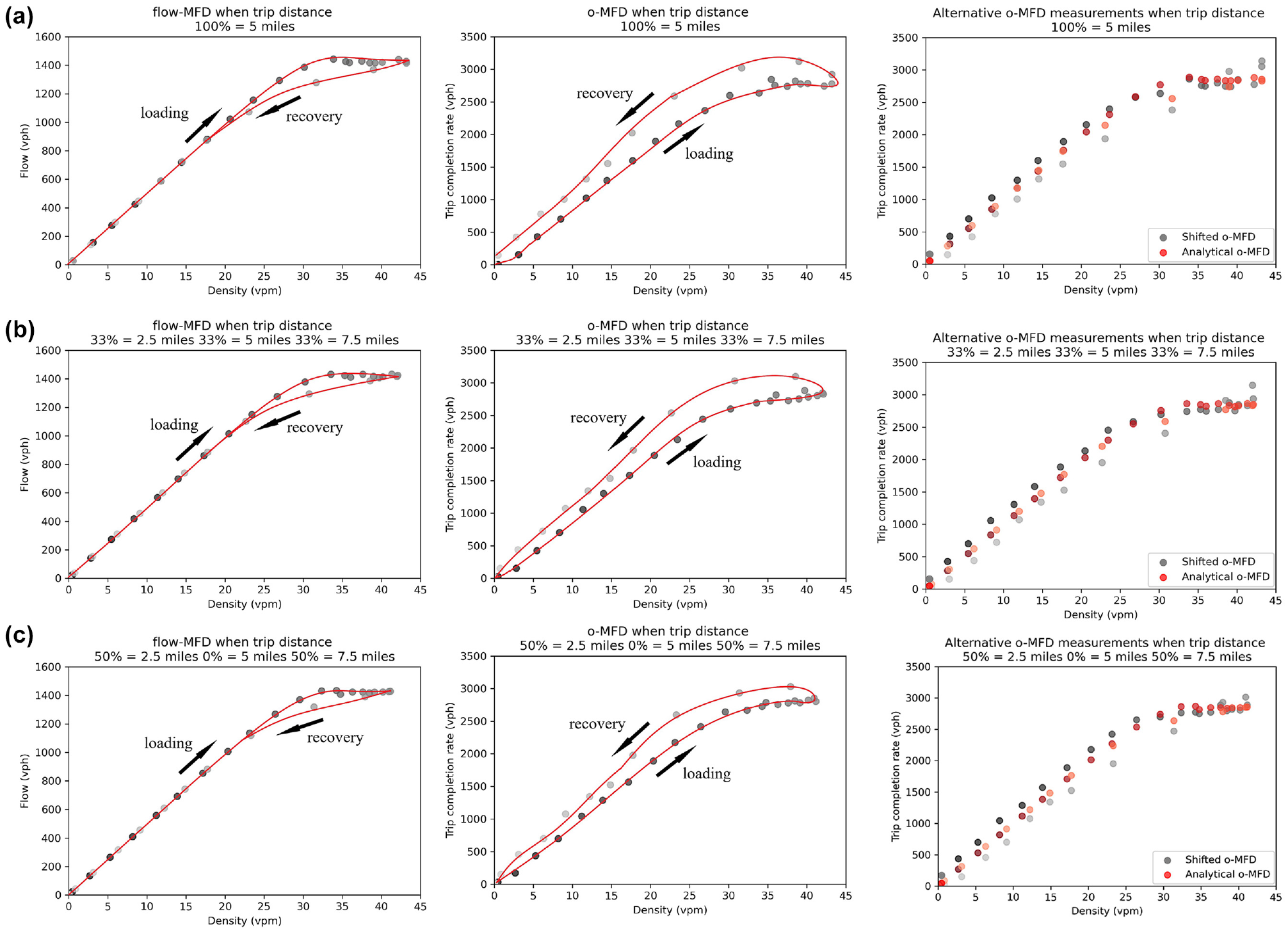
Flow macroscopic fundamental diagram (flow-MFD), outflow macroscopic fundamental diagram (o-MFD), and alternatively measured o-MFD under different randomness of trip distance: (a) trip distance of all vehicles = 5 mi, (b) trip distance of 33.3% vehicles = 2.5 mi, 33.3% vehicles = 5 mi, and 33.3% vehicles = 7.5 mi, and (c) trip distance of 50% vehicles = 2.5 mi and 50% vehicles = 7.5 mi. Darker shades represent measurements performed earlier in time.

Two-Dimensional Grid Network

Simulation Setup

A simulation of a more realistic two-way grid network in AIMSUN is used to investigate the existence of the counter-clockwise loop and figure-eight pattern in the o-MFD. The network simulated here consists of two-way streets arranged into a simple square grid pattern, shown in Figure 13. Each arterial street is 200 m long and consists of two travel lanes which have a free-flow speed of 40 km/h and a capacity of 2,400 vehicles per hour per lane. Intersections are signalized with a signal plan consisting of two phases: one for all movements of eastbound and westbound and the other for all movements of northbound and southbound. The signal has a cycle length of 60 s with an equal green time of 26 s, yellow time of 3 s, and all-red time of 1 s provided to both phases. The signal offsets are set to be 0.

Figure 13.

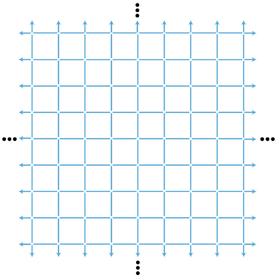
Two-way grid network.

The simulation starts with an empty network. Vehicles gradually enter the network with their ODs located at all intersections (for simplicity). Trips are evenly generated between all OD pairs with an average trip distance of 2 km. The demand follows the profile shown in Figure 8b.

Simulation Results

Range of Trip Distance

We first investigate the impact of the range of trip distance on the hysteresis pattern in flow-MFD and o-MFD. The left side of Figure 14, a and b , provides flow-MFDs obtained from the simulation for trip distance ranging from 1.8 km to 2.2 km and trip distance ranging from 0.2 km to 3.8 km, respectively. As expected, a clear clockwise loop can be observed in the flow-MFD in both cases and the size of the loop increases with the range of the trip distance. The middle column of Figure 14, a and b , provides traditionally measured o-MFDs for each case. It can be seen in Figure 14a that, when the range of trip distance is small, the o-MFD has a clear counter-clockwise hysteresis pattern caused by lag of trip completion because of measurement. By comparison, when range of trip distance is large, the lag of trip completion resulting from the trip distance heterogeneity causes a figure-eight pattern in the o-MFD shown in Figure 14b. These simulation results verify our analytical findings in previous sections.

Figure 14.

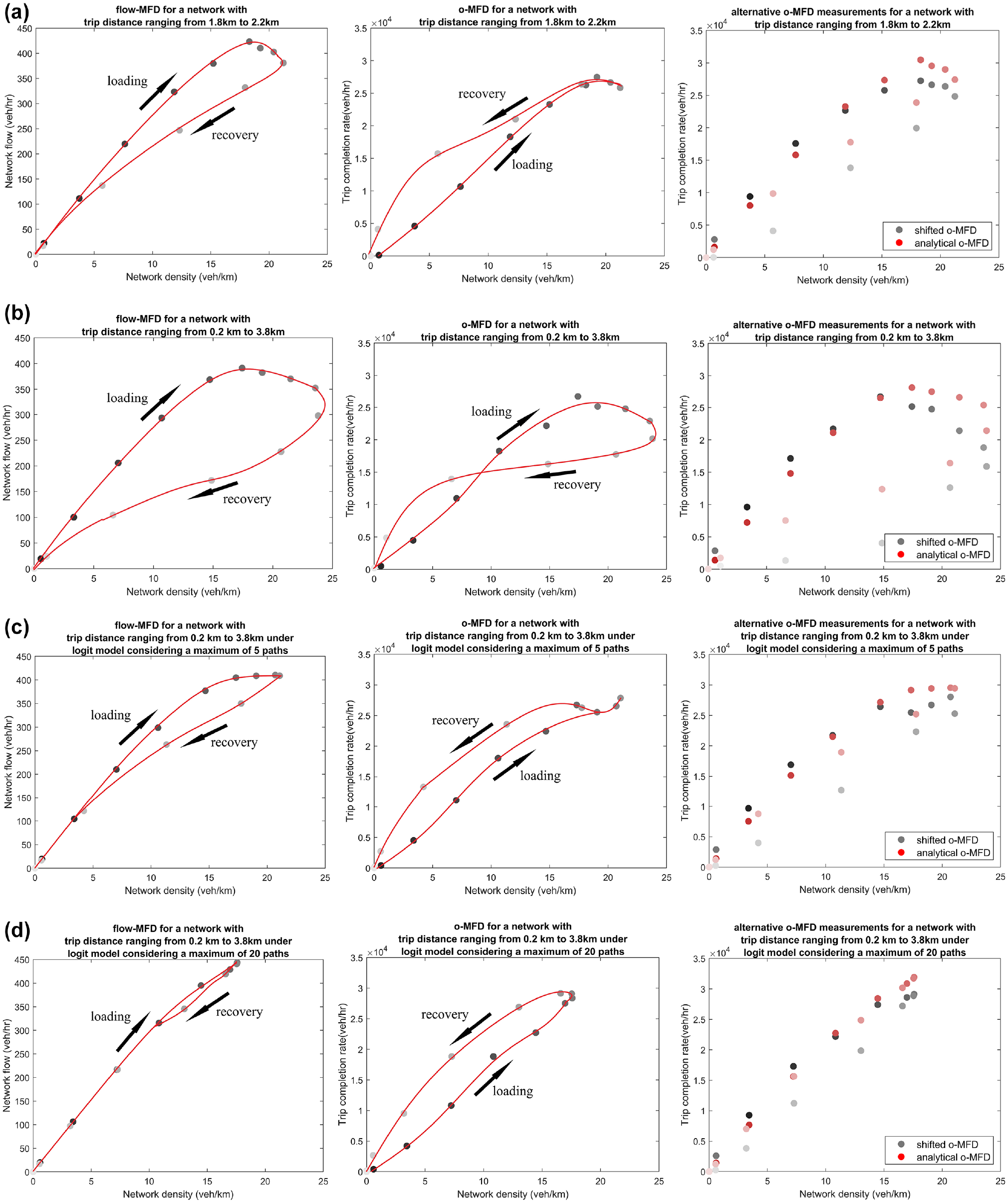
Flow macroscopic fundamental diagram (flow-MFD), outflow macroscopic fundamental diagram (o-MFD), and alternatively measured o-MFD from AIMSUN simulation (a) for trip distance ranging from 1.8 km to 2.2 km, (b) for trip distance ranging from 0.2 km to 3.8 km, (c) under logit model considering a maximum of 5 paths for each trip, and (d) under logit model considering a maximum of 20 paths for each trip. Darker shades represent measurements performed earlier in time.

Driver Adaptivity

Then, we investigate the impact of driver adaptivity on the hysteresis patterns. In Figure 14b, drivers simply take the shortest path and are not adaptive to real-time congestion. By comparison, in Figure 14c, a logit model embedded in AIMSUN is used. Under the logit model, drivers minimize their travel time based on the real-time speed of each road and, thus, are adaptive to real-time congestion. Comparison of flow-MFDs in Figure 14, b and c , reveals that, when drivers choose routes adaptively to avoid congested areas, the network maximum density will decrease and the size of the hysteresis loop will also decrease. Comparison of o-MFDs in Figure 14, b and c , proves that, when drivers are not adaptive to real-time congestion, there can be a figure-eight hysteresis pattern in the o-MFD.

In addition, the impact of route redundancy is investigated by comparing cases in which different maximum numbers of routes are considered in the route choice for each driver. Comparison of Figure 14, c and d , reveals that, when more routes are provided to drivers, the size of the hysteresis loop in the flow-MFD will significantly decrease but the size of the hysteresis loop in the o-MFD will not be greatly affected.

The right side of Figure 14 shows the analytically transformed o-MFD and the shifted o-MFD. As expected, the analytical o-MFDs have the same shape as the flow-MFD on the left side of Figure 14. The shifted o-MFDs no longer have counter-clockwise or figure-eight hysteresis patterns but exhibit clockwise hysteresis loops that are quite similar to the hysteresis loops in the flow-MFD. This indicates a good performance of the “treatment.”

Summary of Findings and Implications

This paper first studies the existence and cause of the hysteresis loop in the o-MFD of general networks under fast-varying demand. While this phenomenon has been previously attributed to the presence of bottlenecks in previous studies, we show here that this arises in the case where no bottlenecks are present using a simple arterial scenario. Instead, the counter-clockwise hysteresis loop in the o-MFD arises because of the delay between vehicles entering and exiting the network. Specifically, vehicles only contribute to the o-MFD when they end their trip. Additionally, since vehicles contribute to the flow-MFD for the entire length of their trip but only to the o-MFD at the end of their trip, this can create opposing hysteresis patterns between the flow- and o-MFDs: the flow-MFD loop is likely to be clockwise because of congestion imbalance growth, while the o-MFD loop is counter-clockwise. Moreover, it is also shown that, when the trip distance heterogeneity causes a lag of trip completion at different locations/exits, a figure-eight pattern can arise in the o-MFD. This paper also provides some empirical evidence that verifies the existence of a counter-clockwise loop and figure-eight pattern in a network’s o-MFD under fast-varying demand.

The impacts of different network features on the size and shapes of these loops are investigated via simulations. The behavior of a ring network is first simulated using CAM. It is found that larger and more rapidly varying traffic demands and longer, less-variable trip distances lead to larger counter-clockwise loops in the o-MFD. Then, a more realistic grid network is simulated in AIMSUM. Results reveal that, when the range of trip distance is small and drivers are more adaptive to congestion, a counter-clockwise hysteresis loop is expected in the o-MFD. By contrast, when the range of trip distance is large and drivers are less adaptive to congestion, a figure-eight pattern will arise in the o-MFD.

A simple approach is proposed for the o-MFD using lagged measurements. The simulation results suggest that this correction produces relationships that are consistent in shape and pattern to the observed flow-MFD. However, further work is needed to ensure that this correction is suitable for practice and is needed on the implications of such a correction. The authors are undertaking this work for a follow-up study.

Overall, this paper contributes to the growing literature on relationships between traffic variables aggregated across large spatial regions and how these relationships are influenced by network features. The results suggest that relationships between the flow-MFD and o-MFD that exist under steady-state conditions—specifically those shown in (1)—are not likely to describe the relationships between these models in dynamic cases, since their overall patterns are so different. This is a significant finding, as very few empirically observed o-MFDs exist in the literature, even though the o-MFD is critical to MFD-based modeling frameworks for the design of regional traffic control studies and other features. Thus, new methods are needed to more accurately estimate o-MFDs in dynamic scenarios so that this tool can accurately describe traffic network dynamics. One promising source is the use of large-scale vehicle trajectory data—for example, the PNEUMA dataset—which can be used to estimate both flow- and o-MFDs ( 39 ). Unfortunately, the PNEUMA dataset contains data for short, non-overlapping periods during the rush and thus cannot provide the o-MFD for an entire, continuous rush period. However, future work should be done to expand on this type of data collection so that researchers have a better understanding of both the o-MFD under dynamic conditions and its relationship to the flow-MFD.

Footnotes

Acknowledgements

This manuscript has been authored in part by UT-Battelle, LLC, under contract DE-AC05-00OR22725 with the U.S. Department of Energy (DOE). The U.S. government retains and the publisher, by accepting the work for publication, acknowledges that the U.S. government retains a non-exclusive, paid-up, irrevocable, world-wide license to publish or reproduce the submitted manuscript version of this work, or allow others to do so, for U.S. government purposes. DOE will provide public access to these results of federally sponsored research in accordance with the DOE Public Access Plan ().

Author Contributions

The authors confirm contribution to the paper as follows: study conception and design: G. Xu, P. Zhang, V. V. Gayah, X. Hu; data collection: G. Xu, P. Zhang, V. V. Gayah, X. Hu; analysis and interpretation of results: G. Xu, P. Zhang, V. V. Gayah, X. Hu; draft manuscript preparation: G. Xu, P. Zhang, V. V. Gayah, X. Hu. All authors reviewed the results and approved the final version of the confirmed.

Declaration of Conflicting Interests

The author(s) declared no potential conflicts of interest with respect to the research, authorship, and/or publication of this article.

Funding

The author(s) disclosed receipt of the following financial support for the research, authorship, and/or publication of this article: This work is supported by NSF Grant CMMI-1749200.

ORCID iDs

Guanhao Xu

Pengxiang Zhang

Vikash V. Gayah

Xianbiao Hu

References

Godfrey

J. W.

The Mechanism of a Road Network. Traffic Engineering & Control, Vol. 11, No. 7, 1969, pp. 323–327.

Mahmassani

Williams

J. C.

Herman

Performance of Urban Traffic Networks. Proc., 10th International Symposium on Transportation and Traffic Theory, Vol. 14, Elsevier Amsterdam, The Netherlands, 1987, pp. 1–20.

Mahmassani

Williams

J. C.

Herman

Investigation of Network-Level Traffic Flow Relationships: Some Simulation Results. Transportation Research Record: Journal of the Transportation Research Board, 1984. 971: 121–130.

Smeed

R. J.

The Road Capacity of City Centers. Traffic Engineering & Control, Vol. 9, No. 7, 1967, pp. 455–458.

Smeed

R. J.

Road Development in Urban Areas. Journal of the Institute of Highway Engineers, Vol. 10, 1963, pp. 5–30.

Thompson

Speeds and Flow of Traffic in Central London. 2: Speed-Flow Relations. Traffic Engineering & Control, Vol. 8, No. 12, 1967, pp. 721–725.

Wardrop

J. G.

Journey Speed and Flow in Central Urban Areas. Traffic Engineering & Control, Vol. 9, 1968, pp. 528–532, 539.

Zahavi

Traffic Performance Evaluation of Road Networks by the α-Relationship. Traffic Engineering & Control, Vol. 14, No. 5–6, 1972, pp. 228–231, 292–293.

Herman

Prigogine

A Two-Fluid Approach to Town Traffic. Science, Vol. 204, No. 4389, 1979, pp. 148–151.

10.

Williams

J. C.

Mahmassani

H. S.

Herman

Analysis of Traffic Network Flow Relations and Two-Fluid Model Parameter Sensitivity. Transportation Research Record: Journal of the Transportation Research Board, 1985. 1005: 95–106.

11.

Geroliminis

Daganzo

C. F.

Existence of Urban-Scale Macroscopic Fundamental Diagrams: Some Experimental Findings. Transportation Research Part B: Methodological, Vol. 42, No. 9, 2008, pp. 759–770.

12.

Geroliminis

Sun

Properties of a Well-Defined Macroscopic Fundamental Diagram for Urban Systems. Transportation Research Part B: Methodological, Vol. 45, No. 3, 2011, pp. 605–617. https://doi.org/10.1016/j.trb.2010.11.004.

13.

Daganzo

C. F.

Gayah

V. V.

Gonzales

E. J.

Macroscopic Relations of Urban Traffic Variables: Bifurcations, Multivaluedness and Instability. Transportation Research Part B: Methodological, Vol. 45, No. 1, 2011, pp. 278–288.

14.

Gayah

V. V.

Daganzo

C. F.

Effects of Turning Maneuvers and Route Choice on a Simple Network. Transportation Research Record: Journal of the Transportation Research Board, 2011. 2249: 15–19.

15.

Mazloumian

Geroliminis

Helbing

The Spatial Variability of Vehicle Densities as Determinant of Urban Network Capacity. Philosophical Transactions of the Royal Society A: Mathematical, Physical and Engineering Sciences, Vol. 368, No. 1928, 2010, pp. 4627–4647.

16.

Gayah

V. V.

Daganzo

C. F.

Clockwise Hysteresis Loops in the Macroscopic Fundamental Diagram: An Effect of Network Instability. Transportation Research Part B: Methodological, Vol. 45, No. 4, 2011, pp. 643–655.

17.

Saberi

Mahmassani

Exploring Properties of Networkwide Flow-Density Relations in a Freeway Network. Transportation Research Record: Journal of the Transportation Research Board, 2012. 2315: 153–163.

18.

Saberi

Zockaie

Mahmassani

Network Capacity, Traffic Instability, and Adaptive Driving: Findings from Simulated Network Experiments. EURO Journal on Transportation and Logistics, Vol. 3, No. 3–4, 2014, pp. 289–308.

19.

Zhang

Garoni

T. M.

de Gier

A Comparative Study of Macroscopic Fundamental Diagrams of Arterial Road Networks Governed by Adaptive Traffic Signal Systems. Transportation Research Part B: Methodological, Vol. 49, 2013, pp. 1–23.

20.

Gayah

V. V.

Gao

X. (Shirley)

Nagle

A. S.

On the Impacts of Locally Adaptive Signal Control on Urban Network Stability and the Macroscopic Fundamental Diagram. Transportation Research Part B: Methodological, Vol. 70, 2014, pp. 255–268. https://doi.org/10.1016/j.trb.2014.09.010.

21.

Ambühl

Loder

Zheng

Axhausen

K. W.

Menendez

Approximative Network Partitioning for MFDs From Stationary Sensor Data. Transportation Research Record: Journal of the Transportation Research Board, 2019. 2673: 94–103.

22.

Luo

Geroliminis

Empirical Observations of Congestion Propagation and Dynamic Partitioning with Probe Data for Large-Scale Systems. Transportation Research Record: Journal of the Transportation Research Board, 2014. 2422: 1–11.

23.

Geroliminis

On the Spatial Partitioning of Urban Transportation Networks. Transportation Research Part B: Methodological, Vol. 46, No. 10, 2012, pp. 1639–1656.

24.

Saeedmanesh

Geroliminis

Clustering of Heterogeneous Networks with Directional Flows Based on “Snake” Similarities. Transportation Research Part B: Methodological, Vol. 91, 2016, pp. 250–269. https://doi.org/10.1016/j.trb.2016.05.008.

25.

Daganzo

C. F.

Urban Gridlock: Macroscopic Modeling and Mitigation Approaches. Transportation Research Part B: Methodological, Vol. 41, No. 1, 2007, pp. 49–62.

26.

Mariotte

Leclercq

Laval

J. A.

Macroscopic Urban Dynamics: Analytical and Numerical Comparisons of Existing Models. Transportation Research Part B: Methodological, Vol. 101, 2017, pp. 245–267. https://doi.org/10.1016/j.trb.2017.04.002.

27.

Lamotte

Geroliminis

The Morning Commute in Urban Areas with Heterogeneous Trip Lengths. Transportation Research Part B: Methodological, Vol. 117, 2018, pp. 794–810. https://doi.org/10.1016/j.trb.2017.08.023.

28.

Leclercq

Paipuri

Macroscopic Traffic Dynamics Under Fast-Varying Demand. Transportation Science, Vol. 53, No. 6, 2019, pp. 1526–1545. https://doi.org/10.1287/trsc.2019.0908.

29.

Sirmatel

I. I.

Tsitsokas

Kouvelas

Geroliminis

Modeling, Estimation, and Control in Large-Scale Urban Road Networks with Remaining Travel Distance Dynamics. Transportation Research Part C: Emerging Technologies, Vol. 128, 2021, P. 103157. https://doi.org/10.1016/j.trc.2021.103157.

30.

Lighthill

M. J.

Whitham

G. B.

On Kinematic Waves. II. A Theory of Traffic Flow on Long Crowded Roads. Proceedings of the Royal Society of London. Series A. Mathematical and Physical Sciences, Vol. 229, No. 1178, 1955, pp. 317–345.

31.

Lighthill

M. J.

Whitham

G. B.

On Kinematic Waves. I. Flood Movement in Long Rivers. Proceedings of the Royal Society of London. Series A. Mathematical and Physical Sciences, Vol. 229, No. 1178, 1955, pp. 281–316.

32.

Richards

P. I.

Shock Waves on the Highway. Operations Research, Vol. 4, No. 1, 1956, pp. 42–51.

33.

Laval

J. A.

Hysteresis in Traffic Flow Revisited: An Improved Measurement Method. Transportation Research Part B: Methodological, Vol. 45, No. 2, 2011, pp. 385–391. https://doi.org/10.1016/j.trb.2010.07.006.

34.

Edie

L. C.

Discussion of Traffic Stream Measurements and Definitions. Proc., 2nd International Symposium on the Theory of Traffic Flow, OECD, Paris, 1965, pp. 139–154.

35.

Han

Ramezani

Hegyi

Yuan

Hoogendoorn

Hierarchical Ramp Metering in Freeways: An Aggregated Modeling and Control Approach. Transportation Research Part C: Emerging Technologies, Vol. 110, 2020, pp. 1–19. https://doi.org/10.1016/j.trc.2019.09.023.

36.

Daganzo

C. F.

In Traffic Flow, Cellular Automata = Kinematic Waves. Transportation Research Part B: Methodological, Vol. 40, No. 5, 2006, pp. 396–403.

37.

Nagel

Schreckenberg

A Cellular Automaton Model for Freeway Traffic. Journal de Physique I, Vol. 2, No. 12, 1992, pp. 2221–2229.

38.

Daganzo

C. F.

On the Macroscopic Stability of Freeway Traffic. Transportation Research Part B: Methodological, Vol. 45, 2011, pp. 782–788. https://doi.org/10.1016/j.trb.2011.02.001.

39.

Barmpounakis

Geroliminis

On the New Era of Urban Traffic Monitoring with Massive Drone Data: The PNEUMA Large-Scale Field Experiment. Transportation Research Part C: Emerging Technologies, Vol. 111, 2020, pp. 50–71. https://doi.org/10.1016/j.trc.2019.11.023.

Opposing Hysteresis Patterns in Flow and Outflow Macroscopic Fundamental Diagrams and Their Implications

Abstract

Keywords

Cause of Counter-Clockwise Hysteresis Patterns in the O-MFD

Measurement Lag

Scenario Setup

Analytical Analysis of Flow-MFD and o-MFD Shape

Trip Distance Heterogeneity

Scenario Setup

Analytical Analysis of Flow-MFD and o-MFD Shape

Empirical Evidence

Shenzhen Nanshan District

Dutch Freeway

Potential Treatment for the Impact of Lags

Impact of Network Features on the Hysteresis Patterns

Ring Network

Simulation Setup

Simulation Results

Peak Demand ( q peak )

Demand Distribution

Randomness of Trip Distance

Two-Dimensional Grid Network

Simulation Setup

Simulation Results

Range of Trip Distance

Driver Adaptivity

Summary of Findings and Implications

Footnotes

Acknowledgements

Author Contributions

Declaration of Conflicting Interests

Funding

ORCID iDs

References

Peak Demand ( $q_{peak}$ )