Sage Journals: Discover world-class research

Abstract

Urban rail transit systems play an essential role in improving mobility and efficiency. A complex rail transit network serves the Boston metropolitan area, U.S., which costs $38 million for the 422 GWh of system electricity consumed annually. With the aim of developing a tool for energy and cost reduction decision support, we propose a comprehensive machine learning framework to investigate line-specific contributions to energy. This effort builds on prior work in estimating a system-wide energy model for the Boston network. By introducing line-specific train movement and operation variables, we obtain a higher-performing model $(R^{2} = 0.91)$ . Furthermore, the model better explains the relationship between energy and train movement, ridership, and weather variables. Most importantly, the model facilitates analyses of how each line contributes to system consumption at the hour level. We found that the non-line-specific variables made a contribution of −2.7% to the average hourly energy of consumption of −5.4 MWh with a baseline energy consumption of 39 MWh. The Red Line dominates the energy consumption among line-specific variables, contributing 2.3% to the hourly average. Our model could be further enhanced to evaluate the energy and cost impacts of line-specific strategies that may be required for future planning and disaster response, as well as for real-time energy monitoring by line.

Keywords

urban rail transit energy modeling random forests ridge regression

With the rapid growth in urbanization worldwide, mobility demand is on the rise in many countries ( 1 ). By 2030, global annual passenger transport volume is estimated to reach 49.7 trillion passenger-miles—an increase of 50% from 2015 ( 2 ). Urban rail transit (URT) systems are an important component of all public transportation modes. According to the American Public Transportation Association, urban rail accounted for 52% of the total ridership miles across all public transit modes between 2019 and 2020 in the U.S. ( 3 ). Globally, the average supply of public transit in developed cities increased from 92 vehicles per kilometer (v/km) in 2001 to 98 v/km in 2012 ( 2 ). Asia experienced rapid growth in URTs with rail length densities (per population size) increasing by 58% between 2005 and 2016 ( 2 ). Meanwhile, the U.S. opened 89 new systems and 135 extensions (rails and subways) from 2000 to 2019. However, the growth in supply and demand has also created challenges concerning energy consumption, as system requirements continue to increase. For instance, URT systems in the U.S. consumed 6.89 GWh of electricity for tractive power in 2019, an increase of 2% from 2018 ( 3 ). This trend underlines the need for strategies to reduce the energy expenditures of URTs for more sustainable outcomes.

Related Work

Several research efforts have investigated models to reduce system-wide energy consumption in URTs. Generally, URT system energy consumption is affected by several variables, such as ridership, temperature, and train schedules, among others ( 4 – 7 ). A comprehensive systems analysis of European URTs identified various dimensions of energy consumption and showed that energy savings of up to 35% could be realized in a URT by optimizing timetables, implementing efficient driving techniques, and installing energy-saving infrastructure ( 8 ). A Petri net modeling approach was also proposed for simulating URT energy consumption and identifying dependencies in power supply and consumption processes. ( 9 ). In an analysis of the North China Plain metro, train frequency was identified as the key factor influencing the system’s energy consumption ( 7 ). A case study on the Beijing Subway demonstrated energy savings of 17.16% via a proposed deep reinforcement learning approach ( 10 ). Another case study on the Beijing Subway showed that an 8% traction energy reduction on a given line could be achieved by optimizing train dwell times ( 11 ). A statistical analysis of onboard train energy data collected over a 4-year period from across Eastern European URTs revealed that the differences in energy consumption across various vehicle types could be as high as 20%, thus highlighting the importance of train replacement or retrofitting as a long-term strategy for energy savings ( 12 ).

At the URT system level, however, there have been relatively few quantitative energy modeling efforts. Notably, linear regression and random forest (RF) models have been shown to be effective in accurately predicting system-wide URT consumption, with Boston used as a case study ( 4 ). However, the limitation of that study lay in the absence of line-specific explanations or predictions. This paper addresses this gap by developing a ridge regression model that, while system-wide, provides line-specific explanations and contributions based on train movement and operations. In addition, the model performs better in prediction than previous models with no line-specificity. This model ultimately has the potential to serve as a decision-support tool for energy reduction strategy exploration and sustainable disaster response and recovery efforts.

We organize the rest of the paper as follows. In the next section, we describe the data sources used in this study. In the Methods section, we describe the framework for generating the line-specific variables and explain the flow of aggregating data. Then, we discuss the models we used to extract features and estimate system-wide energy. In the Results section, we interpret the model parameters and analyze the energy contributions from different categories. Finally, we conclude with key findings and future directions for research.

Data

Study Area

The urban rail transit (URT) system of the Massachusetts Bay Transportation Authority (MBTA) served as the case study. Considered the fourth largest transit agency in the U.S. by ridership, MBTA serviced 1.7 billion passenger miles in the Boston area in 2019 ( 3 ). The four rail lines operating on this network include a light rail line (Green Line) and three heavy rail lines (Red, Orange, and Blue Lines). MBTA spends an average of $38 million on 422 GWh of electricity for the system annually ( 4 ). Table 1 shows detailed information of types and sources of data obtained for the area. We used these to estimate a line-specific system energy model.

Table 1.

Variables and Sources from January 2019 to December 2020

Variable	Source
Timestamped train coordinates	MBTA research database
Hourly energy (MWh)	MBTA official spreadsheets
Hourly temperature (°F)	Metometics database ( 13 )
Hourly precipitation (mm)	Metometics database
Hourly timestamped tap-in ridership	MBTA official spreadsheets

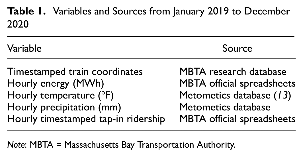
Note: MBTA = Massachusetts Bay Transportation Authority.

Train Location

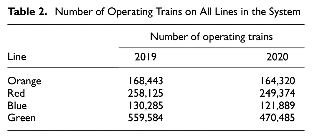
We obtained timestamped train location data from the MBTA-MIT research database for the years 2019 and 2020 ( 4 ). The timestamped data include latitude, longitude, and vehicle identification. The total annual number of operating trains are summarized in Table 2. To illustrate the network, we plot the locations of all timestamp observations for a given day in Figure 1.

Table 2.

Number of Operating Trains on All Lines in the System

Line	Number of operating trains
Line	2019	2020
Orange	168,443	164,320
Red	258,125	249,374
Blue	130,285	121,889
Green	559,584	470,485

Figure 1.

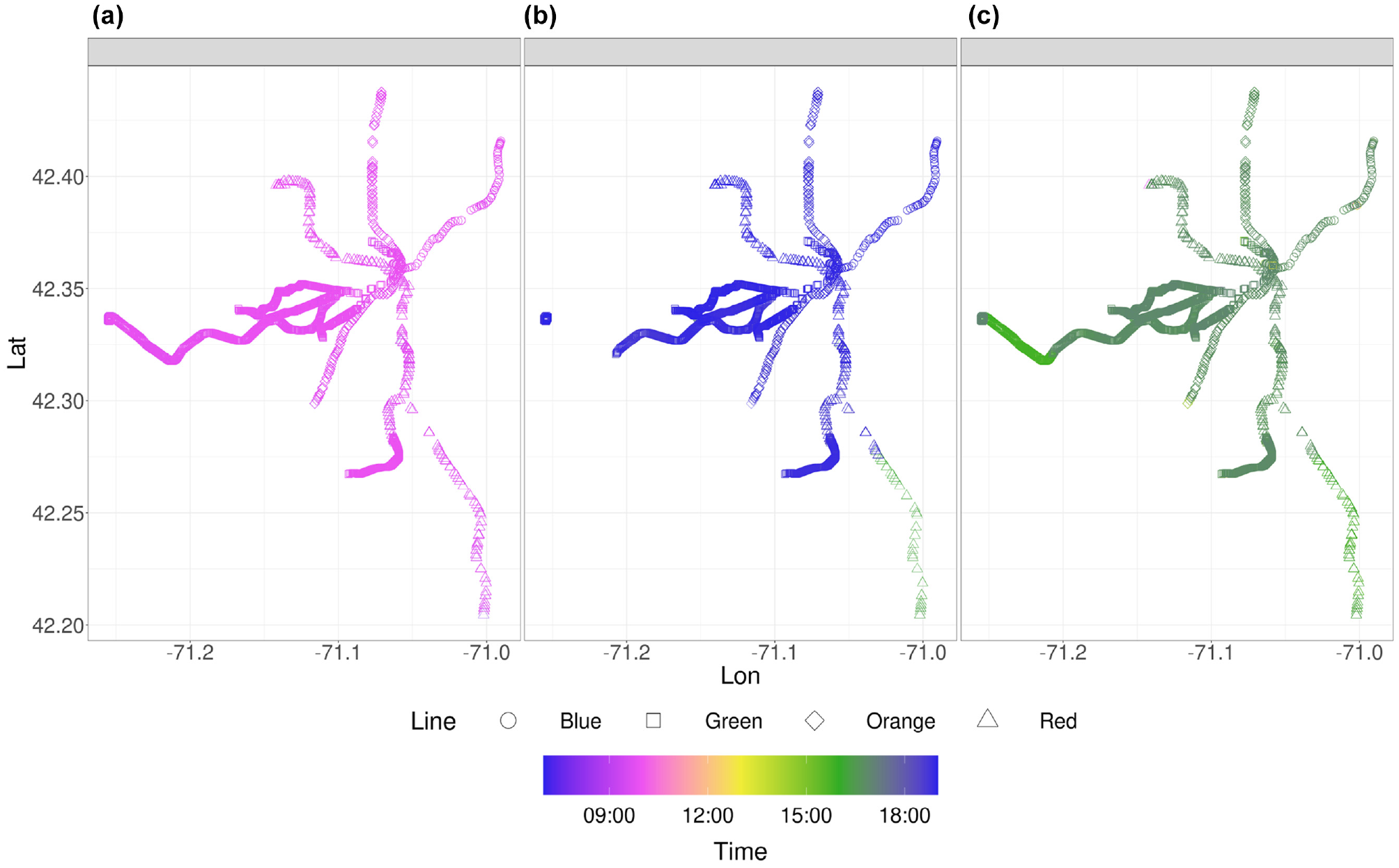
Timestamped locations of trains for the entire day on April 18, 2019: (a) morning peak period (7:00–9:00 a.m.), (b) afternoon peak period (4:00–6:00 p.m.), and (c) off-peak period (9:00 a.m.–4:00 p.m.)

Energy

Hourly energy consumption data from 2019 to 2020 were captured by MBTA’s energy meters across the network (Figure 2). The system’s hourly energy consumption reaches its highest peaks during the winter months (December to February), with an average hourly usage of 53 MWh, indicating the substantial amount of energy used during these months. The hourly average during the non-winter months, however, is 44 MWh. This seasonality pattern (greater energy consumption in the winter compared with the summer) indicates that a significant amount of energy is consumed by heating, ventilation, and air conditioning (HVAC) systems.

Figure 2.

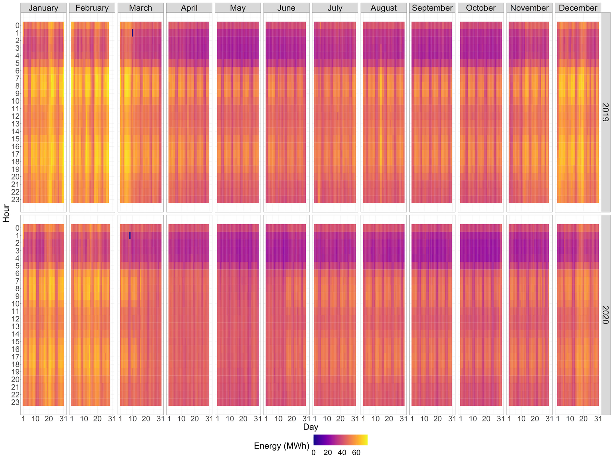
Heatmap of system hourly energy consumption in the Massachusetts Bay Transportation Authority urban rail transit system from 2019 to 2020.

The hourly energy consumption also peaks twice a day (Figure 2), mirroring passenger travel patterns, as well as train schedules. The average hourly energy consumption during the morning peak (7:00–9:00 a.m.) is 54 MWh, while the average afternoon peak (4:00–6:00 p.m.) energy is 55 MWh. During the overnight hours with few train operations, the energy consumption is minimal and the average hourly consumption is only 34 MWh during this period.

Following the COVID-19 lockdown policies implemented in the spring of 2020, MBTA reduced service on the Red, Orange, and Green Lines by 20%, and on the Blue Line by 5% beginning on March 14. These operational changes contributed to a 7.6% reduction in energy consumption in 2020 compared with 2019. This consequently resulted in a decrease of 13.6% in energy costs ( 4 ).

Temperature and Precipitation

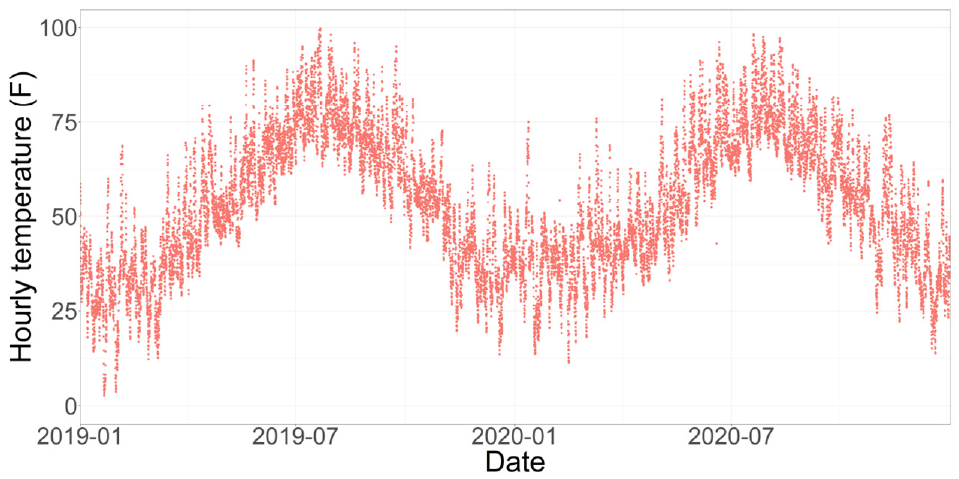
We obtained hourly temperature and precipitation in the Boston area from 2019 to 2020 from the Metometics database ( 13 ). The respective time series are shown in Figures 3 and 4. The highest temperatures (average: $77 ° F$ ) and precipitation (average: 0.2 mm) were recorded in July, while January had the lowest temperatures (average: $33 ° F$ ) and precipitation (average: 0.08 mm).

Figure 3.

Hourly temperature in Boston area from 2019 to 2020.

Figure 4.

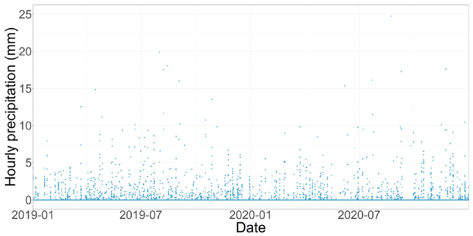
Hourly precipitation in Boston area from 2019 to 2020.

Ridership

We obtained system hourly ridership for 2019 and 2020 from farecard tap-ins recorded in the MBTA-MIT research database (Figure 5). Before the COVID-19 pandemic, the average hourly peak ridership was 15,553. The purple dashed vertical line in Figure 5 indicates the start of the government-instituted COVID-19 lockdown policy, which led to reduced demand and, consequently, service. Although a rebound in ridership was observed after operations resumed in July 2020, the annual hourly peak ridership observed after the lockdown had decreased by 81% compared with the pre-pandemic period.

Figure 5.

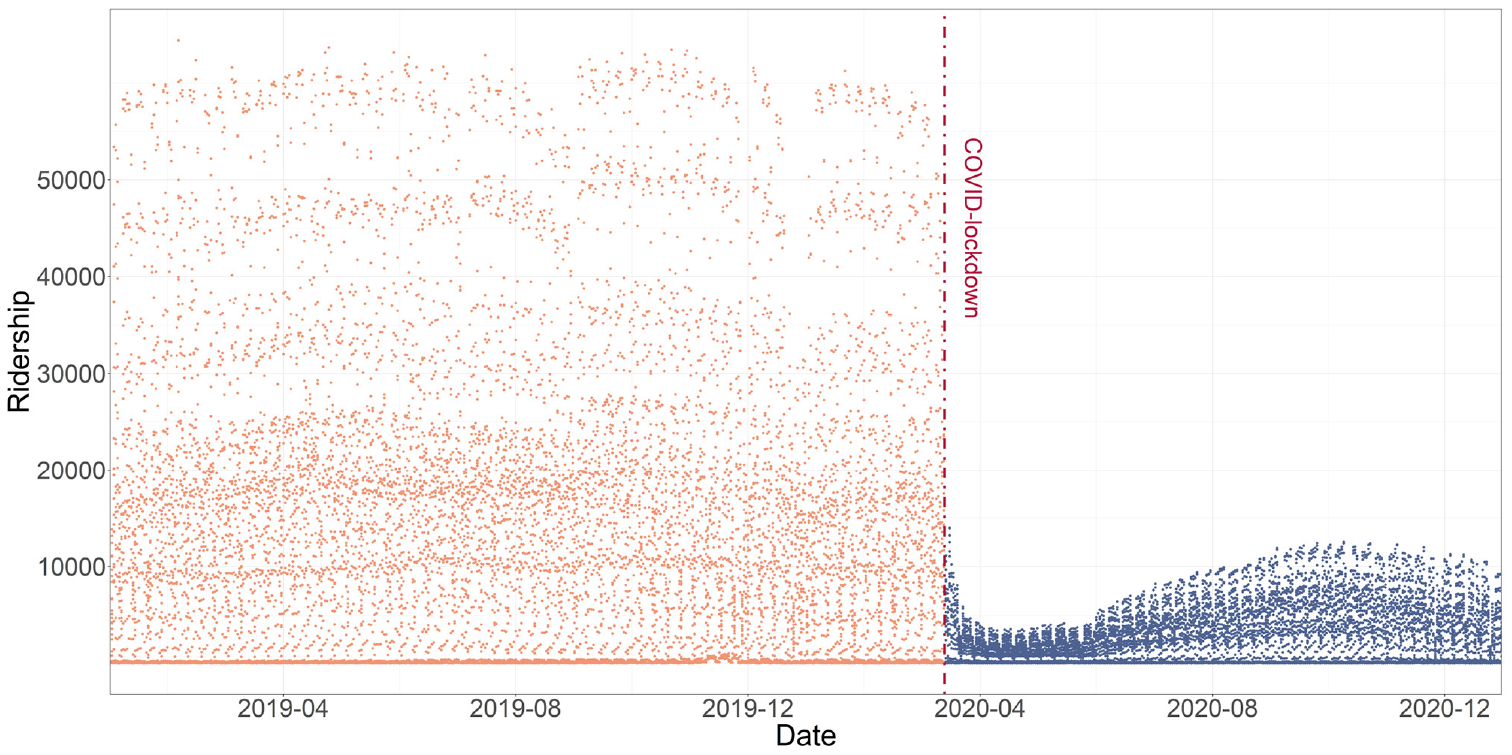
Hourly system ridership in the Massachusetts Bay Transportation Authority (MBTA) urban rail system from 2019 to 2020.

Methods

We computed line-specific trajectories of distance, speed, and acceleration from the high-resolution timestamped locations. Using these, we computed equal probability bin-time variables for speed and acceleration and their interaction at the hourly level to obtain a set of tractive variables. We then aggregated the non-tractive variables at the hourly level and integrated both the tractive and non-tractive variables into an input data set. Using RF models to identify and remove the insignificant variables, we estimated a ridge regression model with the final set of inputs to obtain an interpretable system energy model with line-specific components. The methods are detailed in the following subsections.

Trajectory Computation

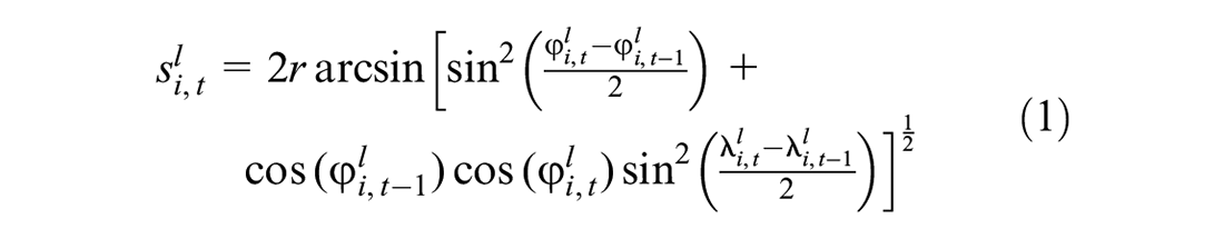
First, we extracted a subset of the train coordinate data set by unique train identification with identical train numbers, vehicle numbers, line labels, and related indicators. Then we sorted the train location by traveling time and computed the operating intervals between two consecutive time location records. We used the Haversine distance function to determine the distance $(s_{i, t})$ between two successive timestamps $t - 1$ and $t$ of each vehicle $i$ ( 14 ). Subsequently, we derived the train trajectory measurements $(v_{i, t}, a_{i, t})$ . The equations used are shown below:

\begin{matrix} s_{i, t}^{l} = 2 r \arcsin [\overset{2}{\sin} (\frac{φ_{i, t}^{l} - φ_{i, t - 1}^{l}}{2}) + \\ {\cos (φ_{i, t - 1}^{l}) \cos (φ_{i, t}^{l}) \overset{2}{\sin} (\frac{λ_{i, t}^{l} - λ_{i, t - 1}^{l}}{2})]}^{\frac{1}{2}} \end{matrix}

(1)

v_{i, t}^{l} = \frac{s_{i, t}^{l}}{Δ t}

(2)

a_{i, t}^{l} = \frac{v_{i, t}^{l} - v_{i, t - 1}^{l}}{Δ t}

(3)

where

$s_{i, t}^{l}$ = distance traveled by vehicle $i$ in line $l$ between timestamps $t - 1$ and $t$ ,

$r$ = radius of the earth,

$φ_{i, t}^{l}$ = latitude of vehicle $i$ in line $l$ at timestamp $t$ (in radians),

$λ_{i, t}^{l}$ = longitude of vehicle $i$ in line $l$ at timestamp $t$ (in radians),

$Δ t$ = time interval between timestamp $t$ and timestamp $t - 1$ ,

$v_{i, t}^{l}$ = average speed of vehicle $i$ in line $l$ at timestamp $t$ , and

$a_{i, t}^{l}$ = average acceleration of vehicle $i$ in line $l$ at timestamp $t$ .

Speed and Acceleration Binning

The tractive energy consumption of a train is governed by the magnitude of its velocity and acceleration ( 15 ). To explore how each line makes contributions to the system energy, we developed a framework to compute the train operating time spent on various speeds and accelerations of each line. Based on the range of calculated speeds and accelerations from the computed trajectories, we find the $k - th$ $q$ -quantiles ${Q_{k}}, k = 1, \dots, q - 1$ , to split the original variable range into equal probability intervals (or bins, $b = 1, \dots, q$ ). We note that $q - 1$ $q$ -quantiles partition a set of observation in a given feature $X$ into $q$ bins. The $q$ -quantile, $Q_{k}$ , generally satisfies the condition:

p (X \leq Q_{k}) = \frac{k}{q}

(4)

More strictly, the $q$ -quantile can be given as ( 16 ):

Q_{k} = inf {x : p (X \leq x) \geq \frac{k}{q}}

(5)

where

inf = the infimum (greatest lower bound) of the set of values ${x}$ satisfying the inequality.

Using line-specific quantiles $Q_{b}^{l}$ and respective bins $b$ , we generated bin-time variables indicating the total amount of time spent by vehicles in line $l$ during hour $h$ . Thus, we define the line-specific speed bin-time $S_{b, h}^{l}$ , acceleration bin-time $A_{b, h}^{l}$ , and speed-acceleration bin time $S_{b, h}^{l} A_{b', h}^{l}$ variables as follows:

S_{b, h}^{l} = {\begin{matrix} \sum_{i, t \in h} Δ_{i, t} I (v_{i, t}^{l} \leq Q_{b}^{l}), & if b < q \\ \sum_{i, t \in h} Δ_{i, t} I (v_{i, t}^{l} > Q_{b - 1}^{l}), & if b = q \end{matrix}

(6)

A_{b, h}^{l} = {\begin{matrix} \sum_{i, t \in h} Δ_{i, t} I (a_{i, t}^{l} \leq Q_{b}^{l}), & if b < q \\ \sum_{i, t \in h} Δ_{i, t} I (a_{i, t}^{l} > Q_{b - 1}^{l}), & if b = q \end{matrix}

(7)

S_{b, h} A_{b', h}^{l} = {\begin{matrix} \sum_{i, t \in h} Δ_{i, t} I (v_{i, t}^{l} \leq Q_{b}^{l}) I (a_{i, t}^{l} \leq Q_{b'}^{l}), \\ if b < q, b' < q' \\ \sum_{i, t \in h} Δ_{i, t} I (v_{i, t}^{l} > Q_{b - 1}^{l}) I (a_{i, t}^{l} > Q_{b' - 1}^{l}), \\ if b = q, b' = q' \end{matrix}

(8)

where

$I (\cdot)$ = the indicator function.

We tested the performance of the RF model (see description in following section) with different numbers of bins as shown in Table 3. For efficiency, we constrained our search to identical bin numbers $q$ and $q'$ , for both speed and acceleration, respectively. The results indicate that the validation out-of-bag (OOB) errors in all cases are similar—ranging from 1.64 to 1.68 MWh. However, taking into account interpretability, we selected the $6 \times 6$ bin case. This enabled us to retain more train movement-related variables while keeping the number of required parameters at a reasonable level. The speed and acceleration quantiles are shown in Figures 6 and 7. This resulted in bins for 36 combinations of speed and acceleration for each line.

Table 3.

Random Forest Model Performance under Different Numbers of Bins.

Bins (Speed × accel.)	Optimal parameters		Out-of-bag error (MWh)
Bins (Speed × accel.)	$n_{T}$	$m$	Out-of-bag error (MWh)
$2 \times 2$	1,000	30	1.68
$4 \times 4$	800	80	1.64
$6 \times 6$	1,000	140	1.68
$8 \times 8$	1,000	200	1.67

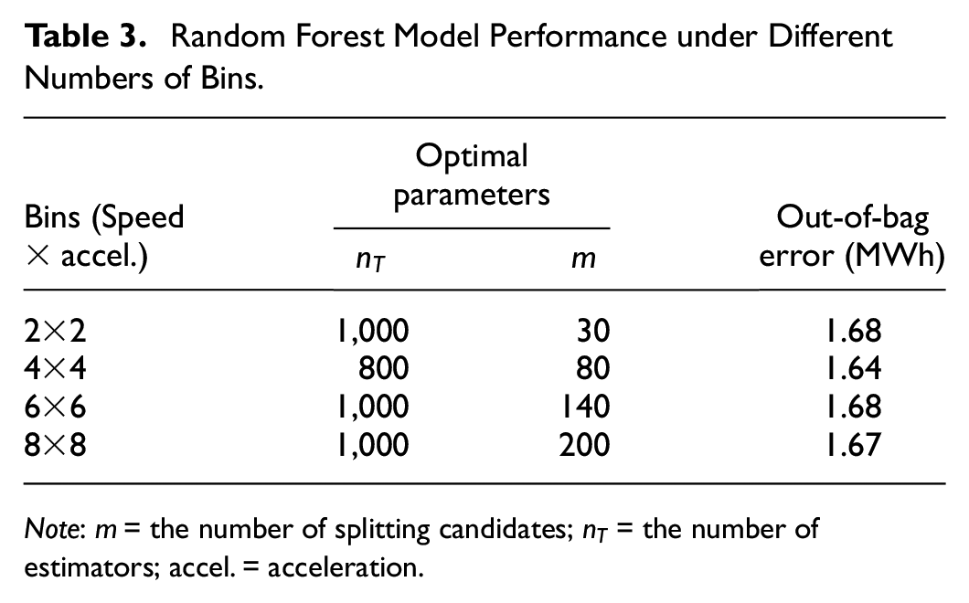
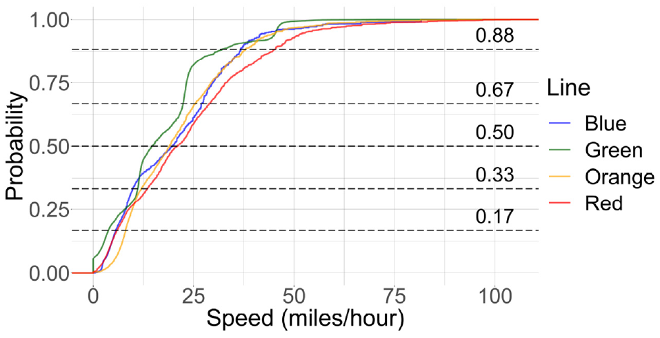
Note: $m$ = the number of splitting candidates; $n_{T}$ = the number of estimators; accel. = acceleration.

Figure 6.

Cumulative distribution function of the computed speeds based on successive observations for each train in 2019.

Figure 7.

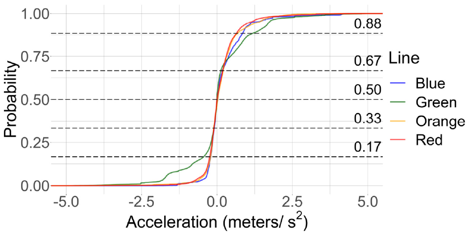
Cumulative distribution function of the computed accelerations based on successive observations for each train in 2019.

Train Operation Variables

We computed the hourly number of operating trains in each line. Figure 8 shows the variation of train operation variables in each line. The Green Line has the busiest schedule which operates an average of 66 trains per hour. Figure 8a reflects the difference of the number of hourly operating trains across different lines. There are twice as many average hourly operating Green Line trains as on the other three lines. Figure 8, b and c , shows the vehicle-hours and vehicle-miles, respectively, for each of the lines. We also observe that the operating hours and distances of the Green Line trains are significantly higher than those of the heavy rail lines.

Figure 8.

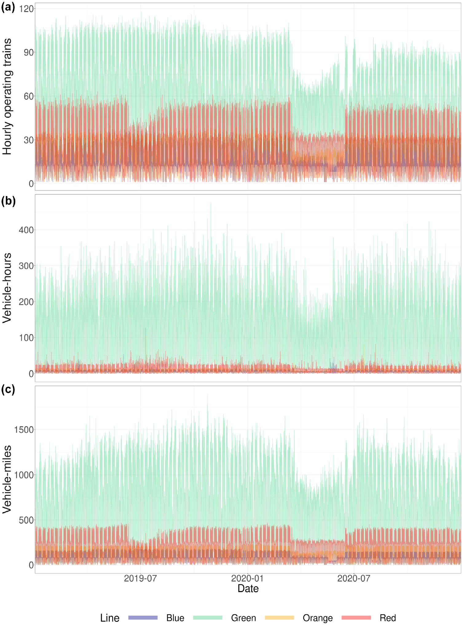
Time series plots of: (a) hourly operating trains, (b) hourly operating time (vehicle-hours), and (c) hourly operating distance (vehicle-miles), from January 2019 through December 2020 for the Massachusetts Bay Transportation Authority urban rail transit system.

Variable Integration

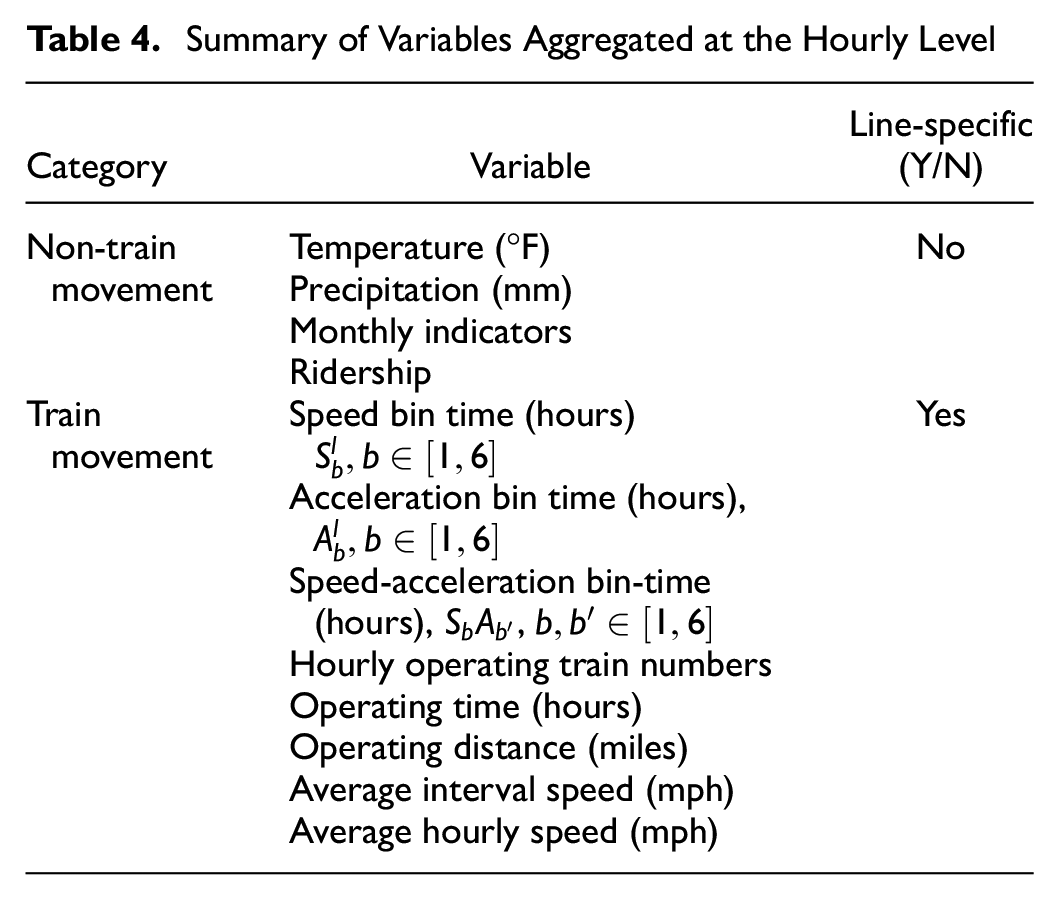
In the previous steps, we obtained the time-stamped vehicle-distances and operating times between two consecutive time records. These computed measurements were summed up at the hourly level to obtain hourly vehicle-distances and operating time. The binning process generated bin-time variables—indicating operating time at various speed, acceleration, and interaction intervals. We also computed hourly operation variables. We then integrated all hourly variables into one single input matrix for model estimation (summarized in Table 4). Overall, 218 variables were processed from the raw data, of which speed bin time, acceleration bin time, speed-acceleration interaction time, and fundamental train movement variables are line-specific. The variables are summarized in Table 4

Table 4.

Summary of Variables Aggregated at the Hourly Level

Category	Variable	Line-specific (Y/N)
Non-train movement	Temperature (°F)	No
	Precipitation (mm)
	Monthly indicators
	Ridership
Train movement	Speed bin time (hours) $S_{b}^{l}, b \in [1, 6]$	Yes
	Acceleration bin time (hours), $A_{b}^{l}, b \in [1, 6]$
	Speed-acceleration bin-time (hours), $S_{b} A_{b'}$ , $b, b' \in [1, 6]$
	Hourly operating train numbers
	Operating time (hours)
	Operating distance (miles)
	Average interval speed (mph)
	Average hourly speed (mph)

Random Forest (RF) Model

We use the RF model to determine the features most relevant to hourly energy consumption ( 17 ). RF is an ensemble method that aggregates predictions from a high number, $n_{T}$ , of decision trees or estimators. In fitting each tree, a random subset of $m$ features is selected at each iteration of the recursive partitioning where the optimal splitting variable and point are found. To find the best-fitting RF model, we performed a $5 \times 7$ grid search over $n_{T} \in {200, 400, \dots, 1000}$ and $m \in {80, 100, \dots, 200}$ , using the OOB error as the objective. In decision tree partitioning, the optimal splitting variable is that which minimizes the node impurity (or maximizes node purity). The accumulated increase in node purity for each variable is then averaged across all the estimators to compute an importance score. By ranking variable importance scores after fitting, we then used the RF model as a feature selector.

Ridge Regression Model

Ridge regression is a linear modeling approach that employs regularization to mitigate overfitting, especially where there is a high number, $D$ , of predictors. The ridge coefficients ${\hat{β}}_{R}$ are given by:

{\hat{β}}_{R} = {(X^{T} X + λ I)}^{- 1} (X^{T} y)

(9)

where

$X$ = the $N \times D$ standardized data matrix,

$λ$ = regularization parameter,

$y$ = $N \times 1$ observed target (hourly energy) vector, and

$N$ = number of observations.

Model predictions $\hat{y}$ are then given by:

\hat{y} = \bar{y} + X {\hat{β}}_{R}

(10)

where the intercept is estimated by the mean response $\bar{y}$ .

We selected the optimal regularization parameter $(λ)$ as 0.6 via 10-fold cross-validation and estimated the ridge regression model based on variables selected via the RF model. From the final ridge regression coefficients, we computed the variable contributions from train movements, weather indicators, and ridership. Thus, we obtained insights into how system energy consumption was distributed across the variables.

We used 70% of the data to train the RF model for selecting the optimal parameters and most-important variables for energy consumption. Then, the same data set was also used to train the ridge regression energy model. We finally used remaining the 30% of variables to test the model performance.

Results

Train Movement Interaction Terms

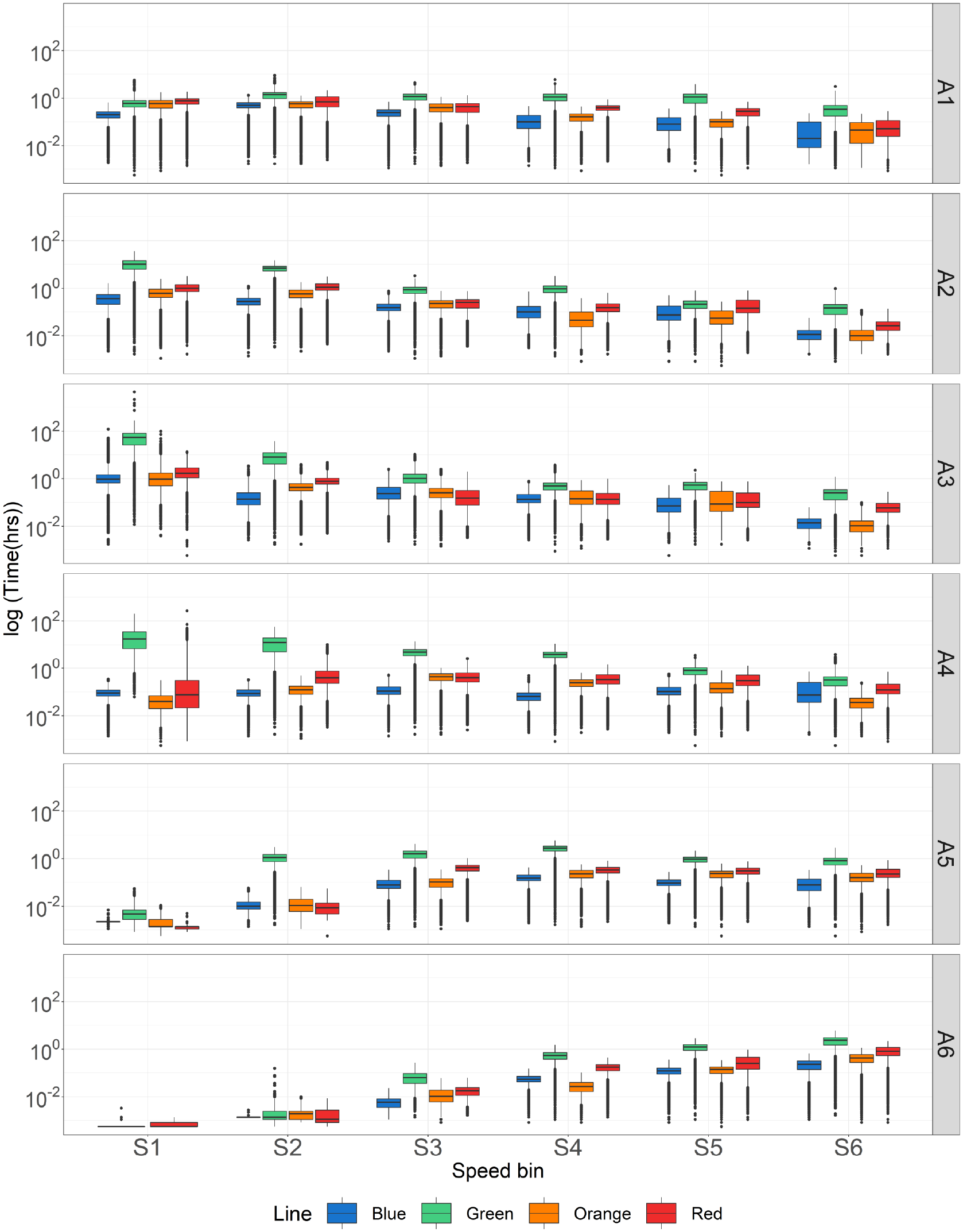
The distribution of the 36 train movement speed-acceleration interaction terms by different lines is shown in Figure 9. We observe that the trains spent more time in the low-speed bins, $S_{1}$ and $S_{2}$ . The Green Line, in particular, accounted for more time than other lines across all interaction bins, as the speed of light rail is lower than that of heavy rail. We also find that the values of interaction terms in low acceleration and low deceleration bins ( $A_{3}$ and $A_{4}$ ) are larger than the terms in medium–high acceleration bins. This shows that trains operated for longer periods with high accelerations. Thus, potentially, energy savings could be achieved via strategies for more efficient driving with lower accelerations.

Figure 9.

Boxplots of log(speed-acceleration interaction time in hours) by speed bin (S1–S6) and acceleration bin (A1–A6).

Feature Extraction

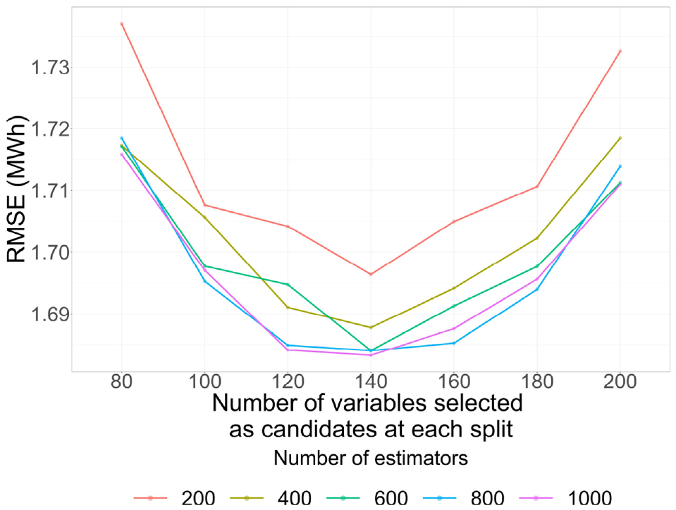
Figure 10 shows the OOB errors for different values of the number of splitting candidates, $m$ , and the number of estimators, $n_{T}$ . The plot indicates that the optimal value for $m^{*}$ is 140, while the optimal number of estimators $n_{T}^{*}$ is 1,000. Thus, we used the RF model with these hyperparameters to investigate feature importance.

Figure 10.

Out-of-bag errors of random forests in the training set for different numbers of estimators $n_{T}$ and number of variables selected as candidates at each split $m$ .

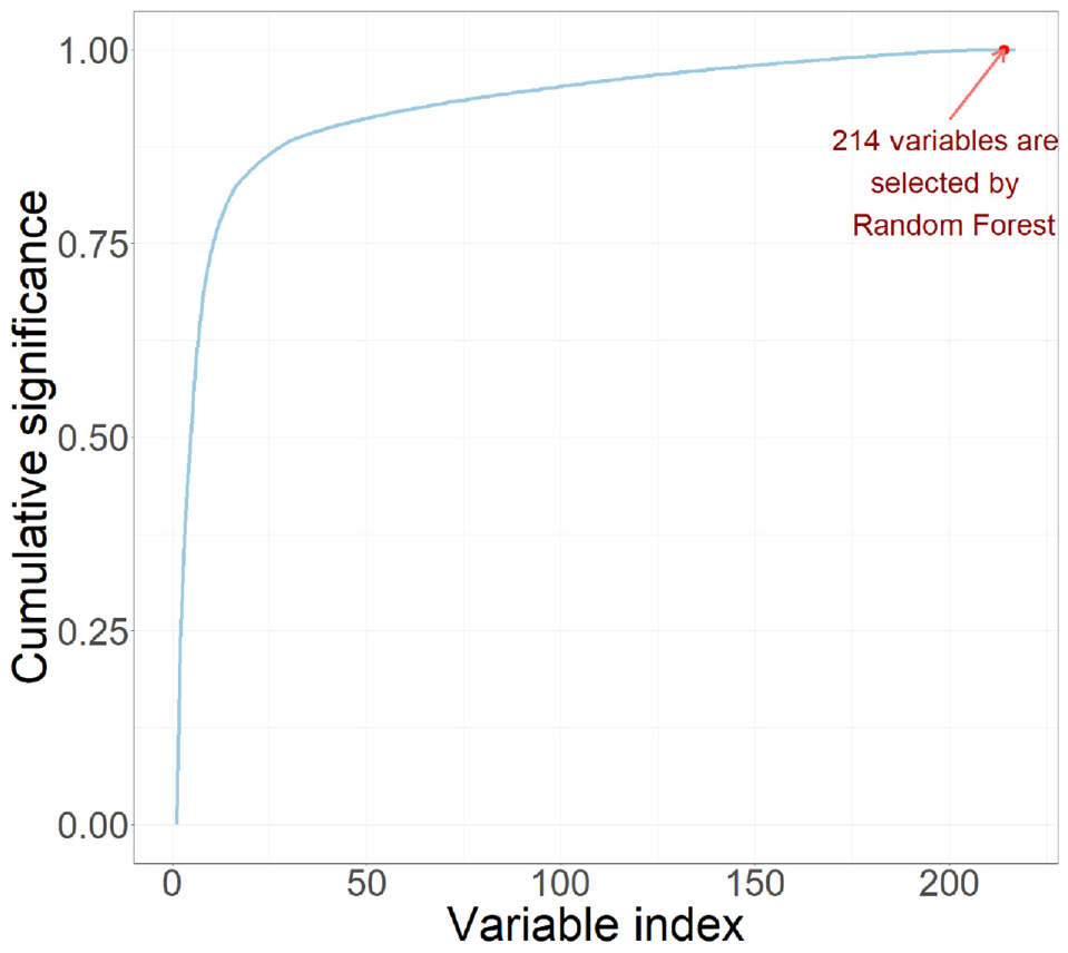
We ranked the importance scores of all variables and then computed the cumulative variable importance (as shown in Figure 11). We observe that cumulative importance increases rapidly by around 35 variables and then the curve begins to flatten, which shows the most significant variables have greater effects on energy consumption. The RF model filtered out the four insignificant variables ( $S_{2} A_{6}^{Red}$ , $S_{1} A_{6}^{Blue}$ , $S_{1} A_{6}^{Green}$ , and $S_{1} A_{6}^{Red}$ ) of 218 variables in the data set. Thus, we selected the other 214 important variables to estimate the system energy.

Figure 11.

Variable importance of random forests in the training set.

Line-Specific System Energy Model

We estimated a line-specific ridge regression model based on the extracted 214 variables. We also assessed its performance on the test set. Figure 12 displays the relationship between predictions and observations. Our model explains 91% of the variance in the training set. In measuring the model performance on the test set, we used the root mean squared error (RMSE) and the mean absolute percentage error (MAPE). We obtained an RMSE of 2.46 MWh and MAPE of 3.95% on the test set, which indicates our model reliably tracks the system energy in the MBTA URT network.

Figure 12.

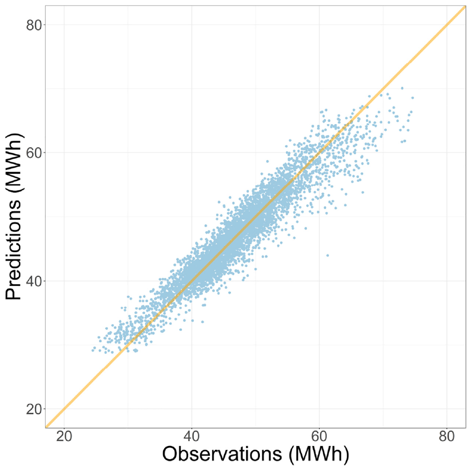
Ridge regression model performance.

Our analysis shows that the hourly energy consumption baseline is 39 MWh, which is possibly because of factors such as signals and station operations. Furthermore, we observed that temperature has a negative coefficient, indicating that, on average, energy consumption increases as temperatures drop (Figure 13). This highlights the importance of HVAC systems. We note that winter months (December through March) contribute significantly to energy consumption, compared with the non-winter months, which on average, save energy (Figure 13). The pattern of the monthly indicators mirrors those of the temperature (Figure 3) and precipitation (Figure 4). This further highlights the significant energy demands of HVAC on the overall system consumption, especially during colder periods.

Figure 13.

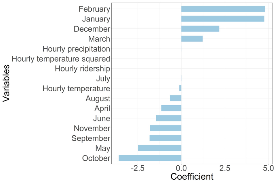
Coefficients of non-line-specific terms (variables named by month stand for the monthly indicators).

Furthermore, we observed a small, negative coefficient for ridership. This can be attributed to the significant decline in ridership following the COVID-19 outbreak, as depicted in Figure 5. Despite the full restoration of train operations (Figure 8) in July 2020, ridership remained at low levels until December 2020. Overall, these findings suggest that both non-tractive factors and the COVID-19 pandemic had a notable impact on energy consumption in the Boston area.

The coefficients of train movement (tractive energy) variables provide a comprehensive overview of how energy consumption varies across different lines in the system. The hourly operating train numbers and operating distances have minimal effects on energy consumption in our model, as tractive energy is explained by the speed and acceleration bin-time variables. Our analysis shows that the Blue Line variables have negative effects on system energy. This could indicate that more Blue Line trains are equipped with regenerative braking compared with other lines, as illustrated in Figure 14. In addition, the average interval speed reflects the average speed of each line over an hour, with small coefficients below 0.006. Similarly, the coefficients for the average hourly speed, which represents instantaneous speed, are also small, with the Red Line having negative effects on energy consumption. This finding could be because the Red Line has the highest speed among the four lines, as depicted in Figure 6.

Figure 14.

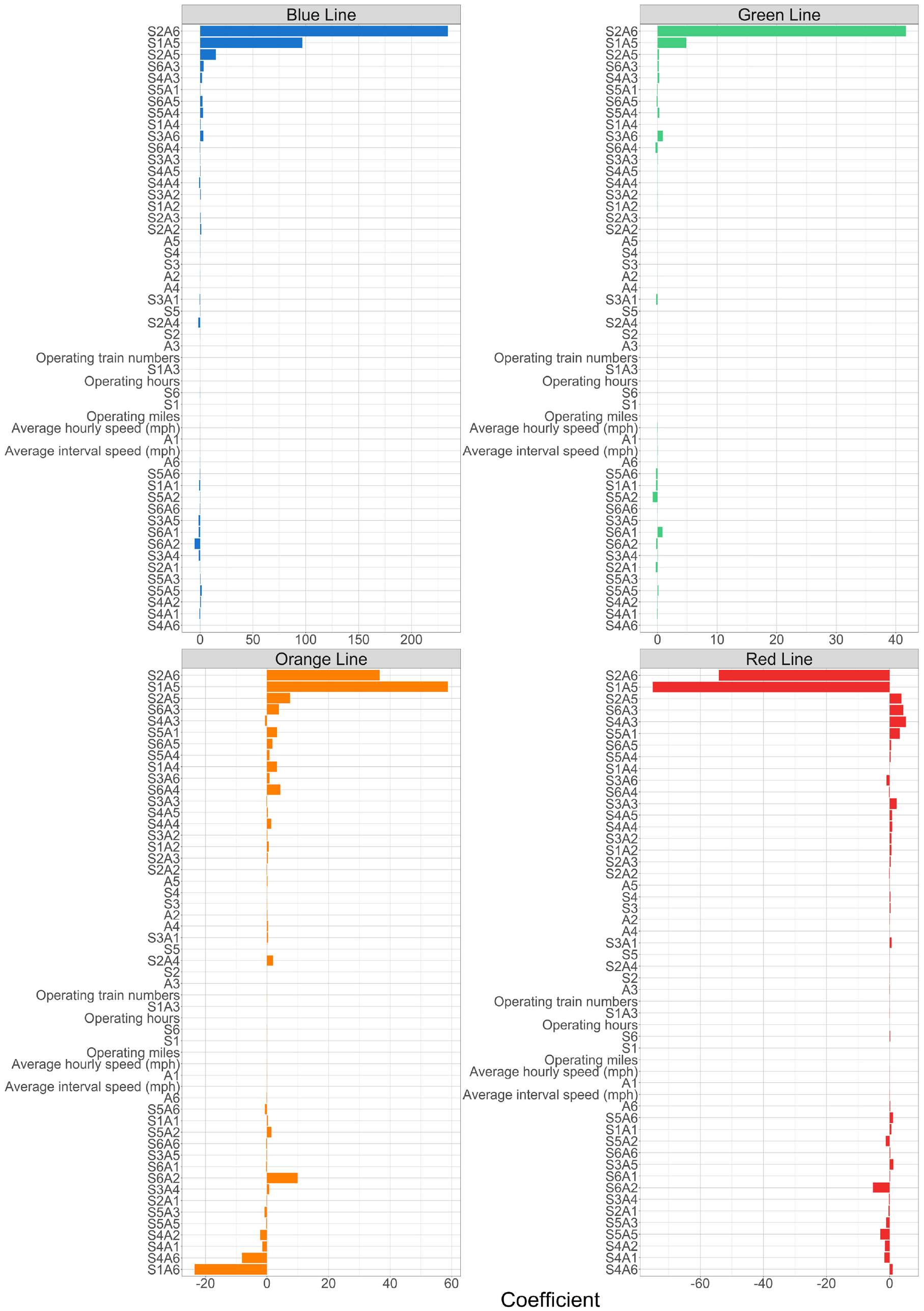
Coefficients of line-specific variables.

The interaction terms can better explain the relationship between system energy consumption and line-specific train movement variables. We found few trains operated within $S_{1} A_{6}$ and $S_{2} A_{6}$ (as shown in Figure 9). Thus, the coefficients of these variables are significantly higher than other interaction terms, as shown in Figure 14. On analyzing the data shown in Figure 9, it can be observed that the mean values of $S_{2} A_{6}^{Red}$ and $S_{1} A_{5}^{Red}$ are lower than those of the other three lines. This finding supports the corresponding negative coefficients observed for these variables. The negative coefficients are potentially correcting for other model discrepancies pertaining to the Red Line. Nevertheless, this behavior will be investigated in future work.

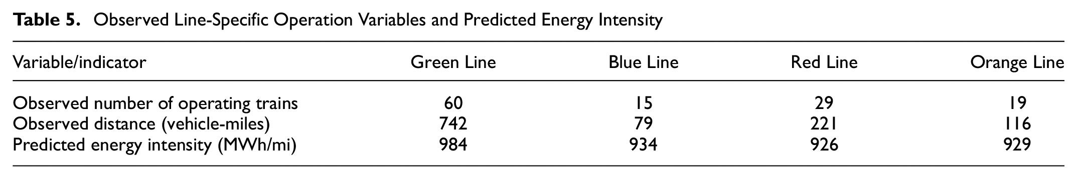
We also observe that interaction bin-time coefficients of the Blue Line at low speeds and large decelerations, such as $S_{6} A_{2}^{Blue}$ and $S_{6} A_{1}^{Blue}$ , all contribute negatively to hourly energy. This is indicative of the prevalence of regenerative braking trains (which harvest energy during deceleration) on the Blue Line compared with the others. Yet, on comparison of predicted energy intensities (MWh per mile), we observe that those of the heavy rail lines range from 926 MWh/mi to 934 MWh/mi (Table 5). The light rail line—Green Line—is the most energy intensive at 984 MWh/mi.

Table 5.

Observed Line-Specific Operation Variables and Predicted Energy Intensity

Variable/indicator	Green Line	Blue Line	Red Line	Orange Line
Observed number of operating trains	60	15	29	19
Observed distance (vehicle-miles)	742	79	221	116
Predicted energy intensity (MWh/mi)	984	934	926	929

Analysis of Energy Contributors

We computed the hourly energy contributions based on the ridge regression predictions and model coefficients, as shown in Figure 15 and Table 6. The non-line-specific variables (temperature, ridership, monthly indicators, and precipitation) contribute an average hourly energy of −5.4 MWh (−2.7%). We observed that the energy contribution pattern of non-train movement variables reflects strong seasonality. The intercept of 39 MWh represents the baseline energy consumption (lights, heating, and cooling, among others).

Figure 15.

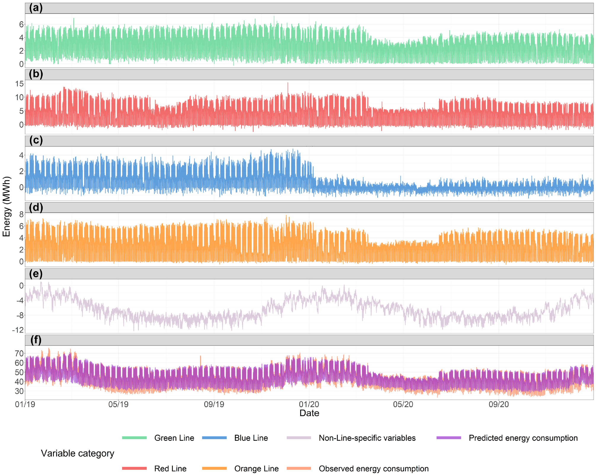
Time series plots of: (a) computed hourly energy contribution of the Green-Line-specific variables, (b) computed hourly energy contribution of the Red-Line-specific variables, (c) computed hourly energy contribution of the Blue-Line-specific variables, (d) computed hourly energy contribution of the Orange-Line-specific variables, (e) computed hourly energy contribution from non-line-specific variables, and (f) comparison on observed energy and predictions from 2019 to 2020.

Table 6.

Hourly Energy Contributions across Different Variable Categories

		Average hourly energy contribution
Variable category		(MWh)	(%)
Intercept		39	97
Non-line-specific		−5.4	−2.7
Line-specific	Green Line	3.04	1.5
	Orange Line	2.90	1.4
	Red Line	4.53	2.3
	Blue Line	0.65	0.3

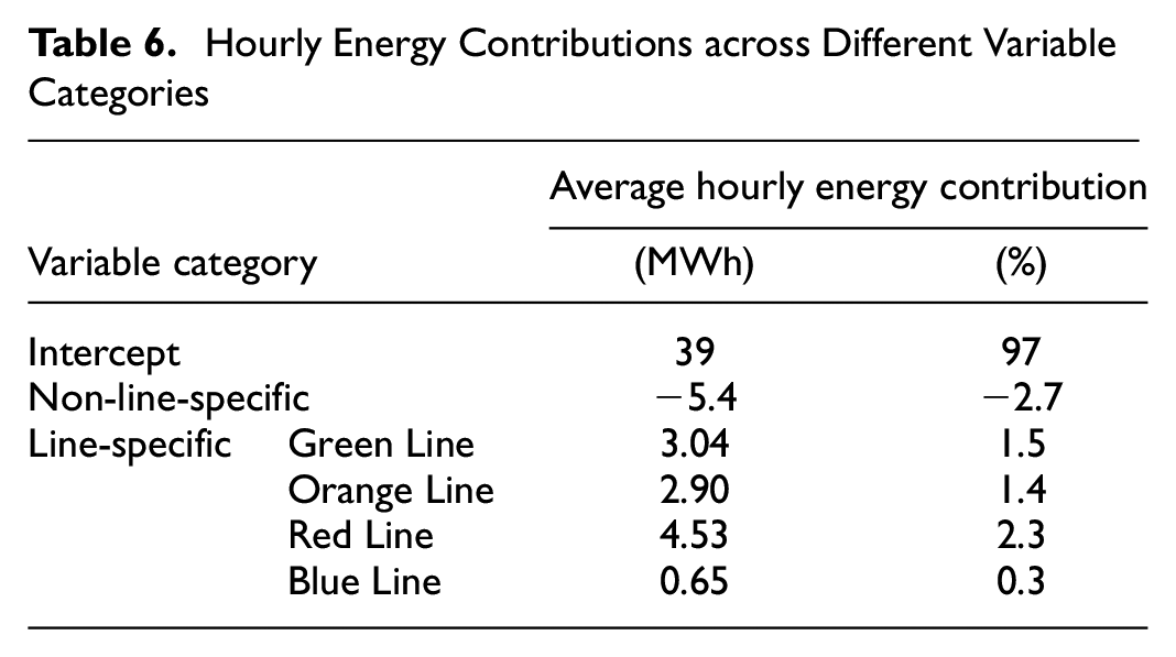
We also captured the energy contributions from line-specific variables as shown in Table 6. Of the four lines, the Red Line accounted for the highest contribution (4.53 MWh) to the average hourly energy consumption. Although the Green Line had the busiest schedule, as shown in Figure 8, it had the second highest contribution from the lines. On average, the Blue Line-specific variables contributed 0.65 MWh to the hourly energy—the lowest of the four. This may be because the Blue Line has the largest proportion of trains with regenerative braking.

Conclusion

The main goal of this study is to explore how the factors of different lines influence system-wide energy consumption. We obtained data on hourly temperature, hourly precipitation, tap-in ridership, and train coordinates from various data sources. To explore the endogenous relationship between energy and train movement, we created different bins for each line to indicate train movement variables under various combinations of speed and acceleration bins. We trained an RF model on 70% data to extract the most relevant variables and then estimated a ridge regression model with the selected variables based on the same training set. The model had an $R^{2}$ of 0.91 and it reliably predicted the energy in the test set with an RMSE of 2.46 MWh and MAPE of 3.95%. The non-train variables made significant contributions to system energy and indicated strong seasonal changes across time. The Red Line dominated the energy contribution among train movement variables and the Blue Line made negative contributions to the energy because it has the largest proportion of trains with regenerative braking.

According to Figure 14, all lines exhibit the highest unit energy consumption under high accelerations at low speeds, except for the Red Line (and only marginally so, as its train spent comparatively much less time in this regime). On the other hand, all lines had significant negative effects on system consumption when accelerating at higher speeds. These observations indicate that energy consumption during acceleration can be divided into two periods. The start-up period will initially require more energy, but, as the trains continue to accelerate, energy consumption will gradually decrease. In comparison to system statistics such as the overall number of operating trains and hours of operation, the interaction terms are more sensitive to the system’s energy consumption.

The strong seasonality of energy consumption was captured in Figures 2 and 15, which motivated us to explore how energy varies across time series. The ongoing research is focusing on estimating a time series model to forecast energy by historical energy observations at different time scales, which depends on the lag we will define in the model. In future work, we plan to train a deep-learning framework to map the low-level movement variables to strategic planning metrics, which could be potentially further used to generate synthetic data.

There are a few potential policy implications of our findings. Our model results indicate that non-movement factors are most significant to system energy consumption. Thus, policymakers might more successfully reduce energy use by focusing on strategies that limit energy use for heating, lighting, signaling, and other non-train operations, instead of reducing transit service. The results of this study specifically reveal that the system consumes more energy in the winter for heating, which could be reduced by installing more insulation. Moreover, the model results indicate that the Blue Line—which has more trains with regenerative braking—made the lowest contributions to the system energy consumption. Increasing the number of trains with regenerative braking may reduce energy consumption.

The data-driven modeling framework developed in this study is highly effective for analyzing any URT system. To predict system energy consumption of a URT, the model relies solely on train location and system-wide energy data, as well as non-line-specific variables listed in Table 4. These variables are readily available from the industrial data set, making the prediction process straightforward. The model must be robust enough to provide accurate information about the energy contributions from all components in the system. Additionally, the model is also able to capture variations in energy consumption caused by factors such as changes in train operations or weather conditions. By carefully designing and testing such a model, we can ensure that it provides accurate and reliable information about energy usage in URT systems, thus enabling more efficient operation and reducing energy consumption. To enhance the interpretability of the model, we will investigate the relationship between the physical model and the estimated machine learning model. Using this approach, the model will not only accurately predict system energy, but also better identify the contributing sources involved. In future research, we plan to validate the impacts of regenerative braking trains on system energy consumption. To achieve this, we will collaborate with URT operators to obtain further line-specific energy data in to validate our model.

Footnotes

Acknowledgements

We would like to thank Sean Donaghy of MBTA for providing the data used in this study.

Author Contributions

The authors confirm their contribution to the paper as follows: study conception and design: J. Oke, E. Christopha, E. Gonzales, Z. Han; data collection: Z. Han; analysis and interpretation of results: Z. Han, J. Oke, E. Christopha, E. Gonzales; draft manuscript preparation: Z. Han, J. Oke. All authors reviewed the results and approved the final version of the manuscript.

Declaration of Conflicting Interests

The author(s) declared no potential conflicts of interest with respect to the research, authorship, and/or publication of this article.

Funding

The author received no financial support for the research, authorship, and/or publication of this article.

ORCID iDs

Zhuo Han

Eric Gonzales

Eleni Christofa

Jimi Oke

Data Accessibility Statement

All the code used in generating the results and figures in this paper are publicly available at . A sample data set is also included for reproducing the methods.

The authors are solely responsible for the facts, the accuracy of the data and analysis, and the views presented here.

References

Oke

J. B.

Aboutaleb

Y. M.

Akkinepally

Azevedo

C. L.

Han

Zegras

P. C.

Ferreira

Ben-Akiva

M. E.

A Novel Global Urban Typology Framework for Sustainable Mobility Futures. Environmental Research Letters, Vol. 14, No. 9, p. 095006. https://doi.org/10.1088/1748-9326/ab22c7

The World Bank. Global Mobility Report: Measuring Progress Toward Safe, Clean, Efficient, and Inclusive Transport. https://www.worldbank.org/en/results/2020/11/11/globalmobility-report-measuring-progress-toward-safe-cleanefficient-and-inclusive-transport, 2017.

American Public Transportation Association. Public Transportation Fact Book. APTA, Washington, D.C., 2021.

Han

Gonzales

Christofa

Oke

Modeling System-Wide Urban Rail Transit Energy Consumption: A Case Study of Boston. Transportation Research Record: Journal of the Transportation Research Board, 2022. 2676: 627–640.

Tang

Yin

Yang

Guo

Predicting the Electricity Consumption of Urban Rail Transit Based on Binary Nonlinear Fitting Regression and Support Vector Regression. Sustainable Cities and Society, Vol. 66, 2021, p. 102690. https://doi.org/10.1016/j.scs.2020.102690

Peng

Wen

Yan

Integrated Optimization on Energy Saving and Quality of Service of Urban Rail Transit System. Journal of Advanced Transportation, 2020, Vol. 2020, p. e3474020. https://doi.org/10.1155/2020/3474020

Guan

Liu

Zhang

Wang

Hourly Energy Consumption Characteristics of Metro Rail Transit: Train Traction Versus Station Operation. Energy and Built Environment, 2022. https://doi.org/10.1016/j.enbenv.2022.05.001

González-Gil

Palacin

Batty

Powell

J. P.

A Systems Approach to Reduce Urban Rail Energy Consumption. Energy Conversion and Management, Vol. 80, 2014, pp. 509–524. https://doi.org/10.1016/j.enconman.2014.01.060

Chenchen

Dongyin

Xuemei

Yanhui

Modeling and Analysis of Global Energy Consumption Process of Urban Rail Transit System Based on Petri net. Journal of Rail Transport Planning & Management, Vol. 21, 2022, p. 100293. https://doi.org/10.1016/j.jrtpm.2021.100293

10.

Yang

Zhu

Lin

Deep-Reinforcement-Learning-Based Energy Management Strategy for Supercapacitor Energy Storage Systems in Urban Rail Transit. IEEE Transactions on Intelligent Transportation Systems, Vol. 22, No. 2, 2021, pp. 1150–1160. https://doi.org/10.1109/TITS.2019.2963785

11.

Lin

Liu

Yang

Zhao

Yang

Sun

Multi-Train Energy Saving for Maximum Usage of Regenerative Energy by Dwell Time Optimization in Urban Rail Transit Using Genetic Algorithm. Energies, Vol. 9, No. 3, 2016, p. 208. https://doi.org/10.3390/en9030208

12.

Ćwil

Bartnik

Jarzębowski

Railway Vehicle Energy Efficiency as a Key Factor in Creating Sustainable Transportation Systems. Energies, Vol. 14, No. 16, 2021, p. 5211. https://doi.org/10.3390/en14165211

13.

Meteomatics. World’s Most Accurate Climate and Weather Data. https://www.meteomatics.com/en/weather-data/, 2022.

14.

Azdy

R. A.

Darnis

Use of Haversine Formula in Finding Distance Between Temporary Shelter and Waste End Processing Sites. Journal of Physics: Conference Series, Vol. 1500, No. 1, 2020; p. 012104. https://doi.org/10.1088/1742-6596/1500/1/012104

15.

Wang

Rakha

H. A.

Electric Train Energy Consumption Modeling. Applied Energy, Vol. 193, 2017, pp. 346–355. https://doi.org/10.1016/j.apenergy.2017.02.058

16.

Wilcox

Chapter 2 -A Foundation for Robust Methods. In Introduction to Robust Estimation and Hypothesis Testing ( R.

Wilcox

, ed.), 4th ed. Statistical Modeling and Decision Science. Academic Press, Amsterdam; Boston, pp. 25–43.

17.

Leo Breiman

Random Forests. Machine Learning, Vol. 45, No. 1, 2001, pp. 5–32. https://doi.org/10.1023/A:1010933404324

Line-Specific Energy Modeling Framework for Urban Rail Transit Systems: A Case Study of Boston

Abstract

Keywords

Related Work

Data

Study Area

Train Location

Energy

Temperature and Precipitation

Ridership

Methods

Trajectory Computation

Speed and Acceleration Binning

Train Operation Variables

Variable Integration

Random Forest (RF) Model

Ridge Regression Model

Results

Train Movement Interaction Terms

Feature Extraction

Line-Specific System Energy Model

Analysis of Energy Contributors

Conclusion

Footnotes

Acknowledgements

Author Contributions

Declaration of Conflicting Interests

Funding

ORCID iDs

Data Accessibility Statement

References