Sage Journals: Discover world-class research

Abstract

Consider a bidirectional arterial road along which several junctions are controlled by fixed-time traffic signals. The driving times between the junctions are far from showing the ideal condition of integer multiples of half the cycle time. At the junctions, separate left-turn phases have to be scheduled. In particular, the two opposite directions of the arterial can but do not need to be scheduled at the same time. This paper provides an integrated mathematical optimization model that maximizes the widths and lengths of the green bands of both directions of the arterial. Within this, the model selects among three predefined signal programs with different phase sequences, and computes optimum offsets for the selected signal programs at each junction. Arranging the left-turn phases before or after the arterial’s through-traffic in a dedicated way provides much better results in the optimization model than always scheduling them at the same time. To validate the optimization result, we implemented a microscopic traffic flow simulation model (using the SUMO simulation package) inspired by certain arterials in the city of Berlin, Germany. With 11 crossings, the result was an average of less than 1.7 stops per car—already including one possible stop at the two entry points of the coordinated arterial. This compares favorably with the average number of at least 3.4 stops per car when the straight traffic in both directions is always scheduled at the same time, that is, in parallel.

Keywords

operations microscopic traffic simulation arterial optimization signal phase traffic light

Despite the availability of traffic-responsive control of street crossings, fixed-time controlled signal programs can still be a matter of choice ( 1 ), in particular, during times that show relatively high traffic volumes in various directions and dense networks with relatively short distances between junctions. When considering one isolated junction (or intersection, or node), there are essentially the following decisions to be taken:

definition of the phases (signal groups that are showing green at the same time),

sequence of the phases, and

lengths of the phases.

When counting any intermediate times as “phases” too, the sum of the lengths of all phases yields the so-called cycle length, after which the very same signal program repeats in a fixed-time control. In practice, given the coordination between neighboring junctions, a common cycle length might be set first, and then the lengths of the phases are computed as fractions of the cycle length (red–green split).

As long as only one direction of traffic flow has to be considered along an arterial, the coordination of a sequence of junctions is simple, because one only has to follow the movement of the first and last cars that can pass at green (and thus, delimit the so-called “platoon” of all cars in between) with their progression speed and propagate their passing times to the subsequent junctions. This may be a viable procedure in the case of a one-way street, or at least if one of the two directions of the traffic flow has a very small traffic volume.

In the more general case where both directions deserve attention, things become more complicated. In particular, in the case of junctions with only two phases, so-called “green waves” typically can only be established in both directions if the well-known driving time condition between two consecutive junctions is met, that is: the driving time equals half of the common cycle length, or some integer multiple of it. Of course, this condition is only rarely met along real-world streets. Even with the best possible coordination (or synchronization) of the relative offsets (or shifts) of the signal programs of subsequent junctions, it is then not possible to establish green waves in both directions.

This is why this paper goes beyond the pure coordination of predefined signal programs. Rather, the aim of this study is to optimize the sequences of the phases, and even select among a predefined small set of alternative phases at each junction.

In the literature, there can be found applications of mathematical optimization for the coordination of traffic lights, even for intermeshed street networks ( 2 , 3 ), involving sophisticated objective functions to measure the waiting times of arriving cars appropriately (Wünsch [ 4 ], in particular, Section 1.3.5). Yet, even for just one given bidirectional arterial in the case where the well-known driving time condition is not met, this approach has to remain limited when the signal programs at the nodes remain fixed.

In the practice of traffic engineering, other methods such as genetic algorithms and simulated annealing algorithms ( 5 ) are also applied. These go beyond the pure inter-node synchronization of predefined fixed signal programs, but make adjustments to the intra-node sequences and even lengths of the phases. However, these algorithmic approaches are not designed to prove optimality, whatever objective function is considered (i.e., minimize the waiting times and/or stops). Gartner et al. ( 6 ) and Zhang et al. ( 7 ) consider decisions of phase sequencing along two arterials that are similar to those studied in the present paper. But in their multi-band and AM-band models, they also take the freedom to adjust the cycle times as well as the progression speeds to compute (at least narrow) green bands along the entire arterial in both directions, and compute their solutions by means of integer linear optimization models. A somewhat different setting of non-overlapping phases for through-traffic, that is, so-called split phases, was considered by Jing et al. ( 8 ) in their Pband model.

Köhler and Strehler ( 9 ) propose a cyclically time-expanded optimization model to compute optimum relative offsets for the fixed signal programs of fixed-time controlled traffic lights, while keeping the phase sequences fixed. In subsequent work ( 10 ), they generalize their model also to select appropriate sequences for the different phases. One instance, for which an optimum solution can usually be found within a few seconds, involves seven junctions, but there is only one cycle in the directed graph, while six junctions are just connected by a unidirectional traffic flow. In contrast, for a larger and intermeshed network of 32 signalized intersections, “a gap of 20 percent between the obtained solution and the lower bound remains when solving this scenario with CPLEX or Gurobi even after hours of computation” ( 10 ).

With this background, the contribution of this paper lies in the combination of:

using compact mathematical models and optimization methods,

broadening their scope to decisions of phase sequencing and even partial selection among a limited number of predefined alternative phases, at the price of,

limiting the use case to arterials (with separate left-turn signal groups) instead of scheduling general road networks, and

finally evaluating the planned results by a microscopic traffic flow simulation.

In addition, our computational results show that allowing for selection among different strategies for the left-turn phases can be highly beneficial. This is supported by an evaluation based on microscopic traffic flow simulation. The mathematical model that is presented in this paper (see also Liebchen [ 11 ]) should be understood merely as an instrument to enable such findings from a traffic engineering point of view. In contrast, tuning the performance of solving the integer linear programs, for example, for longer arterials and/or even intermeshed networks, is left to possible merely mathematical contributions in the future.

To summarize, using the notation of Eom and Kim ( 12 ), the setting considered in this paper has the following properties:

Network type: A (Arterial network)

Real-time strategies: Fixed time

Objectives: TS (Minimization of total vehicle stops, being approximated in the optimization model)

Cycle length: F (Fixed cycle length)

Green phase duration: M, X (green phase duration limited by the same minimum and maximum)

Phase sequence: S (Phase sequence is selected among phase groups).

Basic Setting

The setting is an arterial road along which the left-turn traffic is secured by separate signal groups. For instance, in Berlin, Germany, this scenario applies to several radial road axes in the eastern part of the city (e.g., Prenzlauer Allee), where tramway tracks are located in between the roadways for the inbound and outbound traffic.

A well-established goal for the coordination of subsequent traffic lights along a main street is defined in the German street capacity manual, HBS ( 13 , Sec. S4.4.12):

The quality of the traffic flow in a sequence of coordinated traffic lights can be assessed by a so-called coordination measure k. […] This coordination measure k describes the mean portion of nodes with traffic lights in the coordinated sequence, which can be passed by the cars of the coordinated traffic stream without stop.

While adhering to this “official” goal in the evaluation by simulation, in the mathematical optimization model we approximate this global goal somewhat more locally by maximizing the portion of the entire green interval of an upstream node that arrives at the subsequent node downstream at green. A first reason for the difference between the actual goal and our approximating objective is that the probability for a car to pass the green interval at some node is not distributed uniformly over this interval. Rather, the first seconds of a green interval collect any car that was “stranded” during the red phase (because of lack of coordination, cars entering the arterial from a crossing street, etc.). Moreover, cars do not always drive precisely at the assumed progression speed.

To keep the optimization model local and simple, we refrain from following each car from its entry point to each node of the arterial (see, e.g., Köhler and Strehler [ 10 ]). Otherwise, we would have to detect by appropriate variables in the model down to which subsequent nodes which part of the green interval of the starting node of the path reaches the first, second, third node and so forth downstream without being held at red, see Figure 1. Moreover, if incoming traffic from crossing streets were to be incorporated, these traffic volumes must be available, at least relative to the volume along the arterial.

Figure 1.

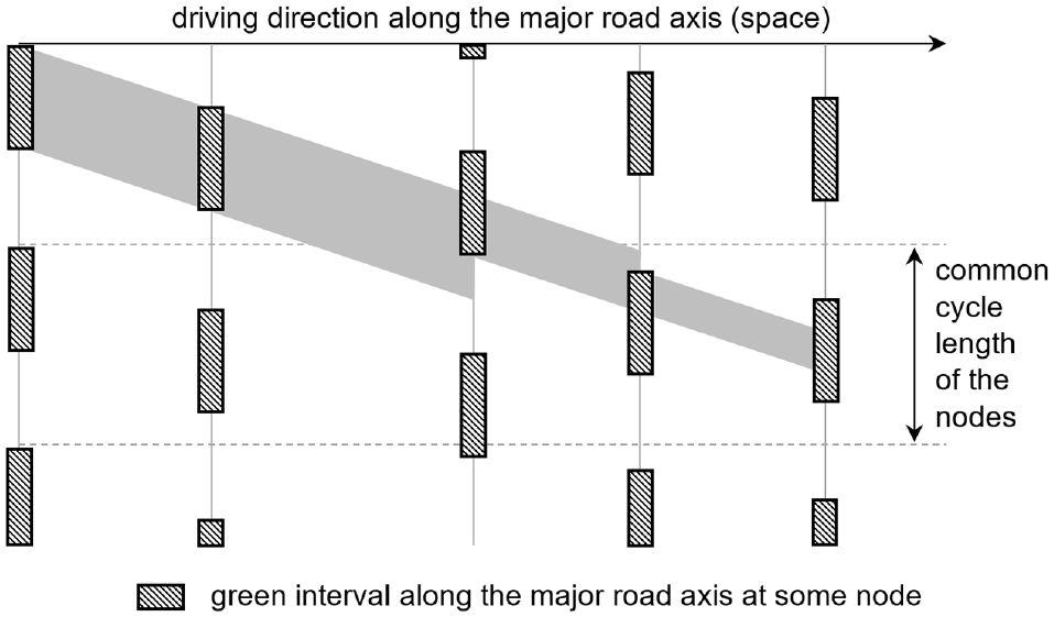
Time–space diagram (time passing top-down) to illustrate the different portions of an initial green interval at the leftmost junction ending in the third and the two next nodes downstream, respectively ( 11 ).

The method for extension of the solution space of the proposed mixed-integer linear mathematical optimization model (MIP) compared with solely optimizing offsets (or shifts) between fixed programs at the junctions is described next. To this end, first, the four relevant basic phases for through-traffic along the arterial and the separate left-turn traffic are shown in Figure 2.

Figure 2.

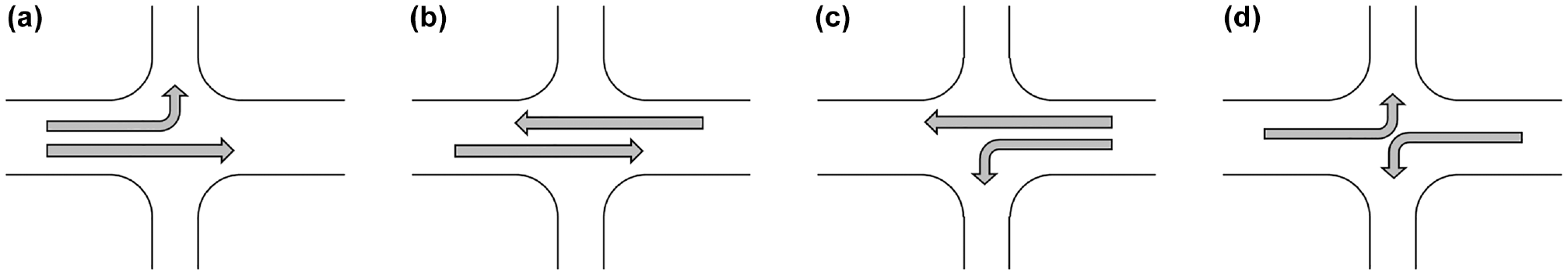
Four relevant basic signal phases for through-traffic along the arterial together with separate left-turn signal groups: (a) west-east through-traffic together with its left-turn phase, (b) parallel through-traffic into both directions along the arterial, (c) east-west through-traffic together with its left-turn phase, (d) both left-turns only.

In the experimental setup, without loss of generality (w.l.o.g.) for the mathematical model, we consider a cycle time of 90 s for all the nodes along the arterial (see also Traffic Signal Timing Manual ( 14 ), Table 6–1). To realize green durations of 50 s for the through-traffic and 15 s for the left-turn traffic, the four combinations and sequences of the four relevant basic phases shown in Table 1 are feasible, but non-uniform green durations at the junctions could also be modeled.

Table 1.

Overview of the Four Relevant Sequences I-IV of the Four Relevant Basic Signal Phases (a)-(d)

Sequence	First phase	Second phase	Third phase	Sum straight	Sum left-turn
I	(a) 15 s	(b) 35 s	(c) 15 s	50 s	15 s
II	(c) 15 s	(b) 35 s	(a) 15 s	50 s	15 s
III	(b) 50 s	(d) 15 s	n/a	50 s	15 s
IV	(d) 15 s	(b) 50 s	n/a	50 s	15 s

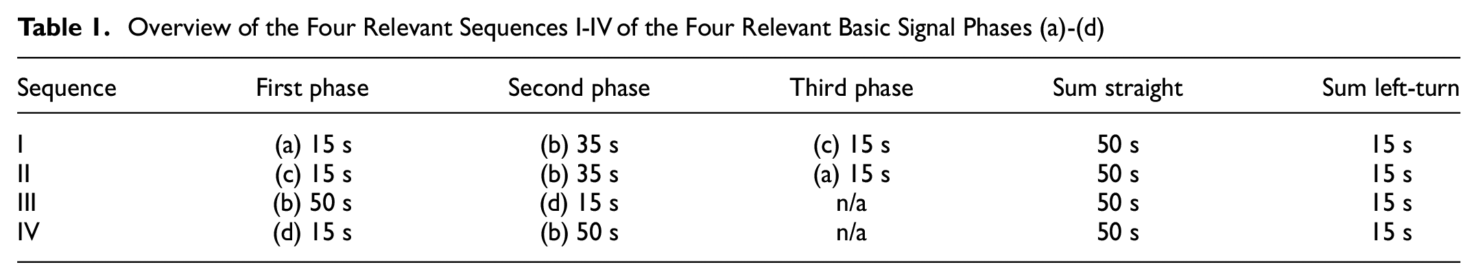
The mathematical optimization model will then select one sequence for each junction, and in an integrated way compute optimum offsets, to maximize the length and the width of the green waves in both directions for the arterial. Of course, Sequence IV will not behave differently for the arterial; for this reason, w.l.o.g. we continue only with Sequences I to III.

As a preliminary, before going into the details of the optimization model, several simplifying assumptions adopted in the mathematical optimization model are listed below:

The model does not count any intermediate times for the changes from one phase to the next during operations (e.g., yellow, all red).

The model does not consider time losses from acceleration or deceleration. In particular, it is beyond the modeling scope of this paper that cars which have to accelerate after they had to wait at red at junction j risk preventing cars that arrive from the previous junction j−1 from continuing without any (slight) deceleration (i.e., queuing).

Apart from prioritizing some first seconds of a platoon, it is essentially assumed that the traffic flow is spread equally over the full length of a green phase.

In particular, when considering the first few seconds of a green phase at junction j as being prioritized when arriving at the next junction j+1, these may fit into the green phase there. However, further downstream their platoon does not need to be part of the prioritized part along the next edge leading to junction j+2 (see also Figure 1).

Notice that during our evaluation using a microscopic traffic flow simulation all of these simplifying assumptions are no longer necessary, and thus will no longer be in place.

Optimization Model

This section essentially follows the presentation in Liebchen ( 11 ), subdividing the presentation of the optimization model into three parts. First, the basic notation used in the model is introduced. Second, it presents the basic structure to compute consistent time values, in particular for the points in time of the beginning of the green phases (node potentials) and for the time durations (e.g., between two junctions or the two opposite directions) (periodic tensions). This basic structure is based on the Periodic Event Scheduling Problem (PESP) introduced in Serafini and Ukovich ( 2 ), also in the context of modeling traffic light signals, and applied for instance in Hassin ( 3 ) and Wünsch ( 4 ). Following that, third, the measurement of certain time durations is described. If a green phase starts a certain number of seconds before or after the upstream platoon arrives, what part of the platoon can pass the junction without having to stop? Quantifying this objective turns out to yield more complex shapes of the objective function than the linear one that is typically applied to periodic tensions when optimizing over a PESP structure.

Notation of Sets and Input Parameters

We are considering an ordered set J = (1,2,…,|J|) of junctions along the arterial to which the optimization model is applied. The two directions of the arterial are D = {WE,EW}, where driving from node j to j+1 shall be from west to east (WE).

The driving time from junction i to junction j, with either j = i+1 in the direction WE or j = i−1 in the direction EW is denoted by d_ij. Next, we consider the duration of the green phase along the arterial. This is assumed to be the same for both directions. To focus on the few first seconds of a green phase—which shall be scheduled preferably without any stop at the next junction with a certain priority—a priority parameter q is introduced for the duration of either the entire green phase (q = “no”) or just the first prioritized seconds (q = “yes”). To conclude, gd_iq denotes the green duration at junction j. In addition, T represents the cycle time that applies to the entire system (e.g., 90 s).

Finally, at each node j, we consider the offset between the possible beginning of the green phase in direction WE and that in direction EW. This offset, or shift, is denoted with s_j. In the above-mentioned Sequences I to III, therefore, we find s_j = 15 s, and thus the green phases of the two directions may be shifted against each other by −15 s, 0 s, or 15 s.

Basic Structure of Variables and Essential Constraints

The periodic events in question are either the starting points of a green phase at junction j in a certain direction, or the points in time when the platoon from the previous upstream junction starts arriving at junction j. The set V of events—or nodes in a graph model—therefore contains two different kinds of beginnings B: green begin nodes GB and arrival begin nodes AB. The actual solution of the optimization model is the values of the node variables in Equation 1,

π_{j, d, b} \in [0, T), j \in J, d \in D and b \in B .

(1)

Notice that the two combinations

j = 1, d = WE and b = AB

j = |J|, d = EW and b = AB

are of no relevance, because the arrival times of the platoons at the first node in their respective direction is beyond the scope of our consideration.

Three types of time durations—or activities, or arcs in a graph model—are considered:

Driving activities A_d, a = (v₁,v₂) ∈ A_d, where v₁ = (j,WE,GB) and v₂ = (j + 1,WE,AB) or v₁ = (j,EW,GB) and v₂ = (j–1,EW,AB);

Offset (shift) activities A_s, a = (v₁,v₂) ∈ A_s, where v₁ = (j,WE,GB) and v₂ = (j,EW,GB), within junction j;

Activities A_w, at the junctions, where cars could face waiting times in case of a stop, a = (v₁,v₂) ∈ A_w, where v₁ = (j,d,AB) and v₂ = (j,d,GB).

See Figure 3 for an illustration of the interplay between vertices and arcs A = A_d∪A_s∪A_w.

Figure 3.

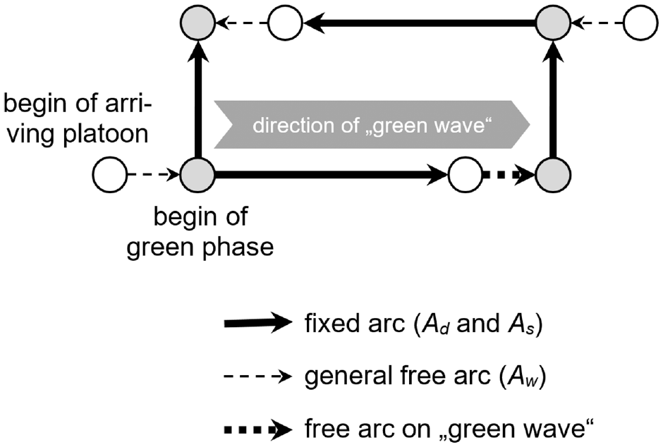
Highlighting the arcs with possible slack along an arterial, where the four leftmost vertices belong to junction j, while the four rightmost vertices belong to junction j+1 ( 11 ).

As is well established when working with PESP-based optimization models, for each arc a = (v₁,v₂) ∈ A we start by considering the pure time difference (aperiodic tension) between the two events v₁ and v₂ and denote it according to Equation 2 (see also Liebchen [ 15 ] 6.26):

y_{a} = {π_{v}}_{2} - {π_{v}}_{1},

(2)

With π_j,d,b ∈ [0, T), the time difference in Equation 2 could become negative. To cope with this, for each arc a ∈ A periodic tension variables x_a are introduced for which an appropriate lower bound ℓ_a ∈ [0, T) and upper bound u_a ∈ [ℓ_a, ℓ_a + T) are defined. This requires Equation 3:

x_{a} \in [ℓ_{a}, u_{a}] .

(3)

The connection between the aperiodic tension variables y_a and the periodic tension variables x_a is established by adding some appropriate integer multiple p_a of the cycle time T, as shown in Equation 4 (see also Liebchen [ 15 ] 6.30), which in fact models the modulo-division operator,

x_{a} = y_{a} + p_{a} \cdot T, for all a \in A .

(4)

The lower and upper bounds for different subsets of the arcs are defined as follows

[ℓ_a, u_a] = [d_ij, d_ij] where a ∈ A_d is the driving activity from junction i to junction j, and

[ℓ_a, u_a] = [0, T−1] for a ∈ A_s.

Since we are only allowing for particular offsets (shifts) to incorporate aspects of phase selection and phase sequencing, the situation for the arc set A_s is slightly more complicated. The general PESP structure is enriched by adding dedicated integer variables and constraints. The possible time differences between the beginnings of the green phases of the two directions at the same junction j are {−s_j, 0, +s_j}. By introducing a variable c_j ∈ {−1, 0, +1}, the expression c_j · s_j immediately provides these three desired possible time differences. Yet, it turns out that the scalings in Equations 1 and 3, respectively, prevent us from simply requiring either y_a = c_j · s_j or x_a = c_j · s_j. Instead, an artificial integer multiplier r_j ∈ {0,1} is introduced to turn the negative value −s_j into T−s_j, and make use of it in Equation 5:

x_{a} = c_{j} \cdot s_{j} \cdot + T \cdot r_{j},

(5)

for all j ∈ J and a ∈ A_s being the offset activity of junction j.

To summarize, the PESP-based model is set up to compute consistent points in time and time durations. The latter consist of directed driving activities between two adjacent junctions, offset (shift) activities between the two directions within the same junction, and activities A_w with possible waiting times along one direction at a junction. It thus remains to weigh the periodic tensions on the arcs A_w by some appropriate objective function.

Objective Function Including Further Constraints

Inspired by the so-called coordination measure of the HBS ( 13 ), this study has the following optimization goal: for each platoon that arrives at a junction, maximize the portion of it that can immediately pass without any stop.

We are aware that the distribution of the cars in an arriving platoon might not be equal. Cars which have just turned from some other crossing street into the arterial will arrive at the next junction at red, if the two junctions are coordinated ideally. We suppose the first seconds of a green phase to contain relatively more cars than later parts of it. Our mathematical optimization model puts particular focus on coordinating the traffic signals such that the first few seconds of an arriving platoon will pass the next junction downstream at green, that is, without any stop. This will be achieved by essentially the same type of objective function that is used to coordinate the entire green phases.

The proposed model is a piecewise linear convex objective function on the arcs of A_w, which the aim of the model is to maximize. This will, of course, require artificial binary variables to separate the different linear parts of the objective function from each other.

Let us start by considering the case of Equation 6, where

g d_{i, no} \leq \frac{T}{2} .

(6)

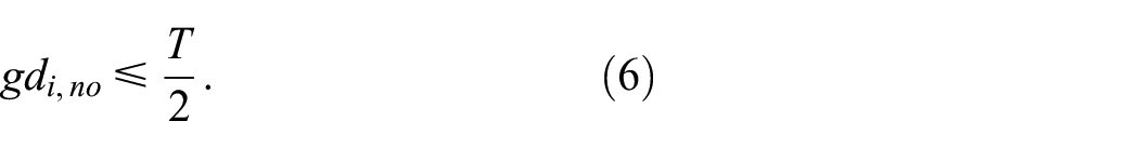
The objective function is presented in Figure 4 and its shape is explained below. The x-axis represents the value of x_a ∈ [0, T), a ∈ A_w, and the value of the objective function is displayed on the ordinate for the example values od gd_i,_no = 30 s and T = 90 s.

Figure 4.

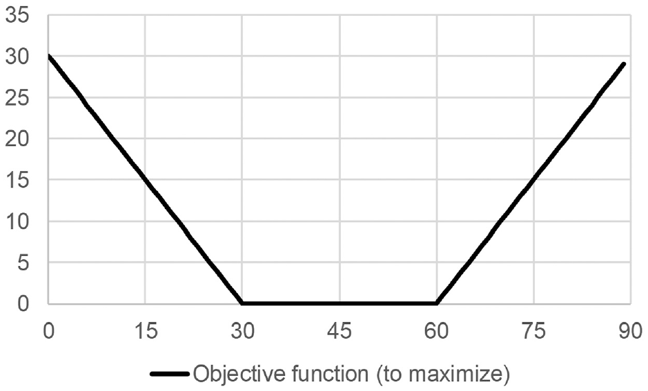
Shape of the piecewise linear convex objective function to be maximized in the case of gd ≤ T/2 ( 11 ).

The value x_a = 0 means that there is no time difference between the beginning of the arriving platoon and the beginning of the green phase at this junction. This is the only relative shift x_a between these two events, where the entire arriving platoon—having length gd_i,_no = 30 s—can continue immediately without any stop, and the objective value may count the full value of gd_i,_no, here 30 s.

Any offset either to the front or to the end will decrease the number of seconds of the arriving platoon that may continue without any stop accordingly. When following the objective function from zero to gd_i,_no or from T−1 to T−gd_i,_no, therefore, it decreases with slope one. Finally, if the offset from the beginning of the arriving platoon to the beginning of the green phase is between gd_i,_no and T−gd_i,_no seconds (recall that we are first considering the case T≥2 gd_i,_no here), then no part of the arriving platoon can continue without stopping, such that the objective function has to remain at value zero.

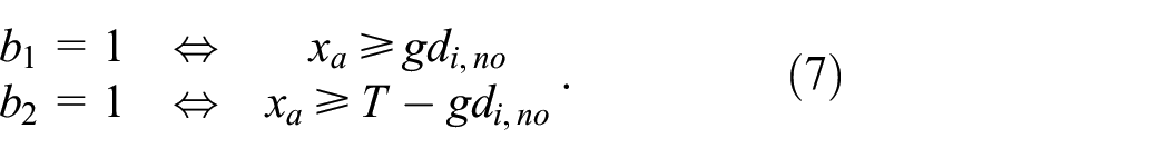
To identify the part of the curve in Figure 4 that is relevant for a given shift x_a, two binary variables, b₁ and b₂, are introduced, see Equation 7:

\begin{matrix} b_{1} = 1 & \Leftrightarrow & x_{a} \geq g d_{i, no} \\ b_{2} = 1 & \Leftrightarrow & x_{a} \geq T - g d_{i, no} \end{matrix} .

(7)

This behavior is obtained by the two pairs of constraints in Equations 8 and 9:

\begin{matrix} x_{a} \leq g d_{i, no} + T \cdot b_{1} \\ x_{a} \geq g d_{i, no} - T \cdot (1 - b_{1}) \end{matrix}

(8)

\begin{matrix} x_{a} \leq T - g d_{i, no} + T \cdot b_{2} \\ x_{a} \geq T - g d_{i, no} - T \cdot (1 - b_{2}) \end{matrix}

(9)

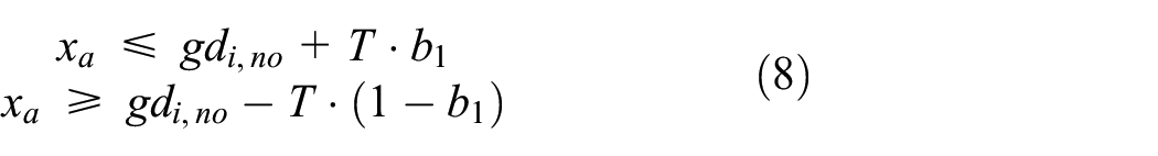
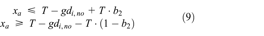
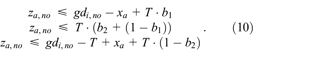
Observe that the value T is playing the role of a “big M value” to (de-)activate the respective constraints depending on the actual value of b₁ and b₂. Finally, we introduce a variable z_a,_no to model the actual value of the maximization objective function, that is, the y-value in Figure 4, whose upper bound shape is divided into three linear parts, according to Equation 10.

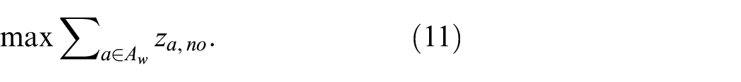
\begin{matrix} z_{a, no} \leq g d_{i, no} - x_{a} + T \cdot b_{1} \\ z_{a, no} \leq T \cdot (b_{2} + (1 - b_{1})) \\ z_{a, no} \leq g d_{i, no} - T + x_{a} + T \cdot (1 - b_{2}) \end{matrix} .

(10)

The objective function then simply turns out to be the term in Equation 11:

max \sum_{a \in A_{w}} z_{a, no} .

(11)

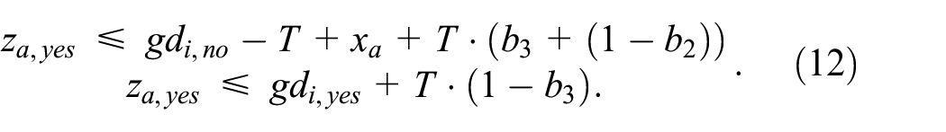
In the alternative case of q = “no” but gd_i,_no ∈ [T/2, T), the graph of the objective function is still divided into three piecewise linear segments. But the middle part does not have a value of zero, but rather 2 gd_i,_no−T; see Liebchen ( 11 ) for further details. Finally, to set up the objective function variable z_a,_yes accordingly, we again simply introduce a third artificial binary variable b₃ with b₃ = 1 ⇔x_a≥T−(gd_i,_no−gd_i,_yes) and finally replace the last inequality in Equation 10 and add one for the last interval, where z_a,_yes = gd_i,_yes, see Equation 12:

\begin{matrix} z_{a, yes} \leq g d_{i, no} - T + x_{a} + T \cdot (b_{3} + (1 - b_{2})) \\ z_{a, yes} \leq g d_{i, yes} + T \cdot (1 - b_{3}) . \end{matrix} .

(12)

Data Set

The study area is a 3 km long bidirectional arterial with two lanes each for driving in both directions. Along this arterial, there are 11 junctions, where separate left-turn lanes always ensure that at least one through lane will not be blocked by any turning cars. This situation is similar to several major road axes in the city of Berlin, for example, Prenzlauer Allee. As on several other streets in Berlin, there is a tramway line in the middle between the two roadways for the two directions. To provide safe left turns from the arterial, there are separate green phases, when the trams have to stop, see Figure 5. In both parts of it, the left signal (white bars) is the special signal for the tramway, the signal in the middle (left arrows) applies to the left-turn traffic, and the signal on the right is for the straight traffic that continues along the arterial. In the left part of the figure, the special signal for the tramway (white vertical bar) gives allowance for the tramway in parallel to the straight traffic, while the left-turn arrow is showing red, see Phase (b) in Figure 2. In contrast, in the right part of the figure, the tramway has to stop (white horizontal bar) so that there is no conflict with the green arrow for the left-turn traffic, see Phase (a) in Figure 2.

Figure 5.

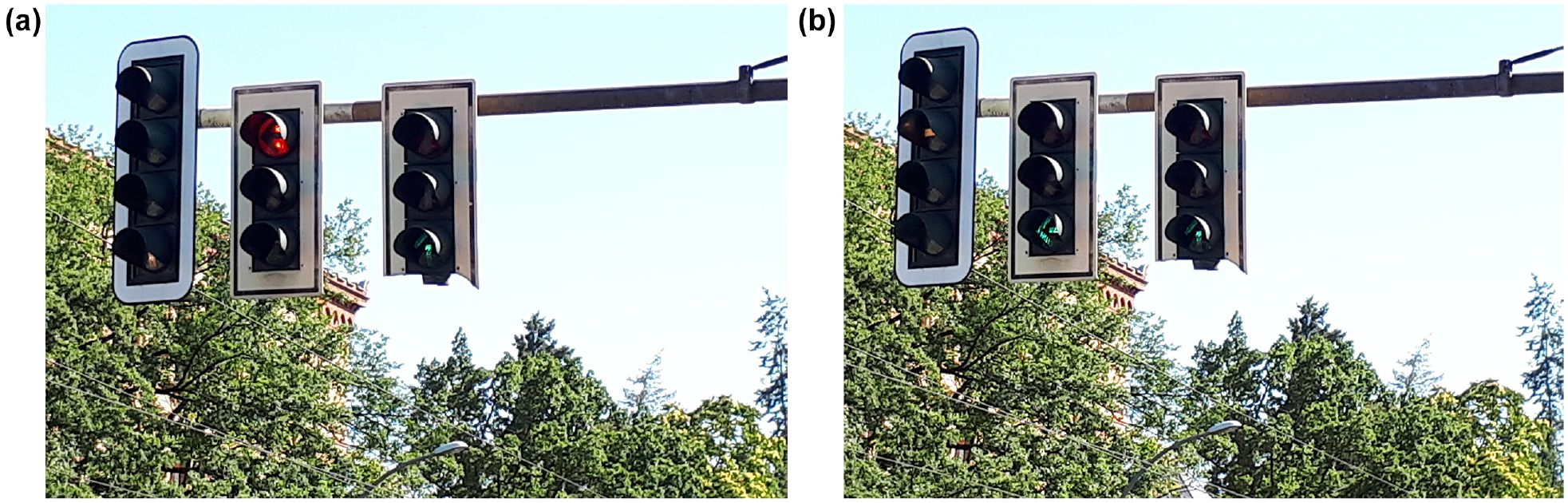
Traffic light signals to ensure safe left turns from an arterial with a tramway line in between the two roadways on Prenzlauer Allee, Berlin: (a) corresponds to fig. 2 (b); (b) corresponds to fig. 2 (a) or (c).

We assume a cycle time of T = 90 s, as it is often used in Germany. For the straight traffic along the arterial, the green phase duration is 47 s, plus a yellow phase of 3 s. For the left turns, we schedule 12 s of green, again plus a yellow phase of 3 s. For the sake of completeness, let us mention explicitly that the crossing roads have 22 s of green, plus the 3 s yellow phase.

To demonstrate the full potential of the proposed integer linear optimization model, we avoid the ideal driving times of half the cycle time (i.e., 45 s) and integer multiples of it. Figure 6 depicts the driving times (in seconds) between two adjacent junctions. Although only the interplay between driving times and the cycle time is relevant, the total driving time of 200 s could be translated to a distance of 3 km (corresponding to the 10 segments between Torstraße and Ostseestraße along Prenzlauer Allee), when assuming an average free flow progression speed of about 15 m/s (54 km/h), which can be typically measured when the allowed maximum speed is 50 km/h.

Figure 6.

Visualization of the driving times (in seconds) between two adjacent junctions along the bidirectional arterial.

Next, in Table 2, observe that even when summing the driving times for up to six consecutive road segments, there are only five entries that show values in a ±5 s interval around an integer multiple of half the cycle time (in particular 45 s, 90 s, or 135 s), as shown in bold italic.

Table 2.

Partial Sums of the Driving Times in Figure 6

From/to	2	3	4	5	6	7	8	9	10	11
1	20	48	72	84	96	120	148	168	184	200
2	-	28	52	64	76	100	128	148	164	180
3	-	-	24	36	48	72	100	120	136	152
4	-	-	-	12	24	48	76	96	112	128
5	-	-	-	-	12	36	64	84	100	116
6	-	-	-	-	-	24	52	72	88	104
7	-	-	-	-	-	-	28	48	64	80
8	-	-	-	-	-	-	-	20	36	52
9	-	-	-	-	-	-	-	-	16	32
10	-	-	-	-	-	-	–		-	16

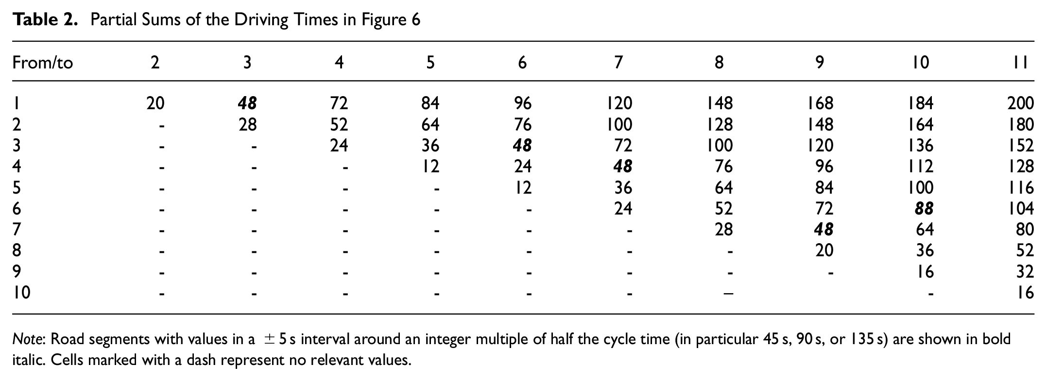
Note: Road segments with values in a ±5 s interval around an integer multiple of half the cycle time (in particular 45 s, 90 s, or 135 s) are shown in bold italic. Cells marked with a dash represent no relevant values.

With these values, the computational study will indeed show that if at each junction the times of the green phases of both directions are precisely the same, that is, c_j = 0, then the quality of the coordination probably has to remain limited.

Optimization Results

Recall that the following parameters in the mathematical optimization model must be set to some value to perform a computation:

the length of the prioritized green duration gd_j,_yes,

the degree of freedom whether both directions must have green at the very same time (i.e., c_j = 0), or if we may select the phase sequence at each junction independently from any other junction (i.e., c_j ∈ {–1,0,+1}). Since Liebchen ( 11 ) did not report any truly interesting solutions if the same pattern c_j should apply to each junction, we omit this setting for the present series of computations,

the requirement whether an ideal green wave in one direction (w.l.o.g., WE) has to be established (i.e., x_a = 0, for a ∈ A_w in direction d = WE), and

global objective weights by which the sum over q = yes and q = no may be weighted by either 1 or 10.

Within the optimization model, we optimize the objective function (Equation 11). Still by only using the variables that are defined in the optimization model, we also report the fraction (in percent) of

\sum_{d \in {WE, EW}} \sum_{j \in J} g d_{j, q}, q \in {yes, no}

(13)

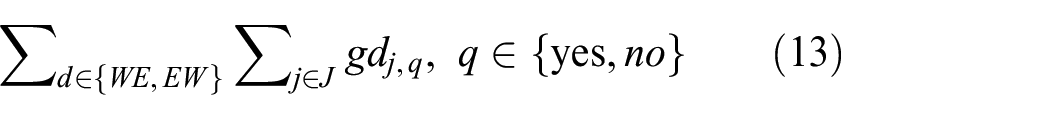
which the proposed model is could attain as hypothetical maximum value. Later, in the evaluation with the simulation model, the average number of stops of the cars, per direction, as well as the time loss that the cars are facing on average along the arterial, will serve as the main performance indicators that are reported.

The computational results that are reported in Table 3 were obtained on an Intel Core i5-5200U at 2.20 GHz with 8 GB RAM, where the mathematical optimization model was implemented in AIMMS 4.86.6.2 and finally solved with CPLEX 20.1. The reference value for q = no is computed by multiplying for both directions the maximum possible width of the green band (50 s) that can pass at one of the 10 junctions (the first uncoordinated one being excluded) without having to stop, that is, 2 · 50 · 10 = 1,000.

Table 3.

Computational Results of the Mathematical Optimization Model

ID	gd_j ,_yes	Objective weight for q=yes	Objective weight for q=no	Sequence requirement	Green wave WE?	Computation time (s)	Solution quality for q=yes	Solution quality for q=no
	10			(reference)			200 (100%)	1,000 (100%)
03	10	10	1	c_j = 0	no	2.1	200 (100%)	600 (60%)
07	10	1	10	c_j = 0	no	20.9	164 (82%)	660 (66%)
11	10	10	1	c_j ∈ {−1,0,+1}	yes	0.9	192 (96%)	794 (79%)
13	10	10	1	c_j ∈ {−1,0,+1}	no	9.5	192 (96%)	794 (79%)
15	10	1	10	c_j ∈ {−1,0,+1}	yes	3.8	172 (86%)	846 (85%)
17	10	1	10	c_j ∈ {−1,0,+1}	no	6,346.1	172 (86%)	846 (85%)
	25			(reference)			500 (100%)	1,000 (100%)
02	25	10	1	c_j = 0	yes	0.1	360 (72%)	660 (66%)
04	25	10	1	c_j = 0	no	2.8	488 (98%)	600 (60%)
08	25	1	10	c_j = 0	no	40.8	404 (81%)	660 (66%)
12	25	10	1	c_j ∈ {−1,0,+1}	yes	0.8	469 (94%)	794 (79%)
14	25	10	1	c_j ∈ {−1,0,+1}	no	3.6	492 (98%)	794 (79%)
16	25	1	10	c_j ∈ {−1,0,+1}	yes	1.6	442 (88%)	846 (85%)
18	25	1	10	c_j ∈ {−1,0,+1}	no	5,903.2	442 (88%)	846 (85%)

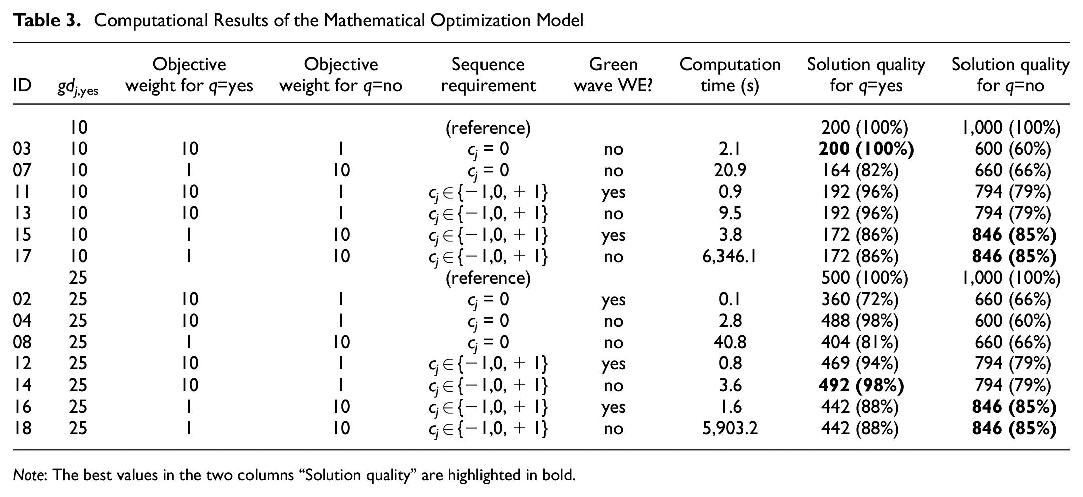
Note: The best values in the two columns “Solution quality” are highlighted in bold.

Before reporting the quality of the signal plans according to the simulation runs, let us briefly point to three details. First, in the combination of both c_j = 0 and “green wave WE” equal to “yes”, the entire plan (ID02) becomes fixed. Thus, we refrain from reporting the same row in the table for gd_j,_yes. Second, in particular in cases with objective weight for q = “no” equal to 10, the fact that the solution quality for q = “no” (in both directions together) is the same no matter whether we require a priori a green wave WE or not (i.e., ID15 versus ID17, and ID16 versus ID18), just mirrors the proposition of Theorem 1 in Liebchen ( 11 ). Third, consider the solution behavior for ID18. The chart in Figure 7 reports the evolution of the quality of both the primal solution and the dual bound during the branch and bound process. Similar to the findings of Lindner and Liebchen ( 16 ) for a pure PESP model, the optimum solution is found relatively early (after 47 s), while the optimality proof is only available after 5,903 s. Recall that large duality gaps are also reported in Köhler and Strehler ( 9 ).

Figure 7.

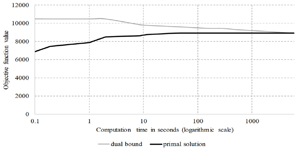
Computational performance of the mixed-integer linear programming (MIP) solver. An optimum solution has been found after 47 s, while after 2,000 s still an optimality gap of 2% pertained and optimality is proved only after 5,903 s.

Simulation Setup

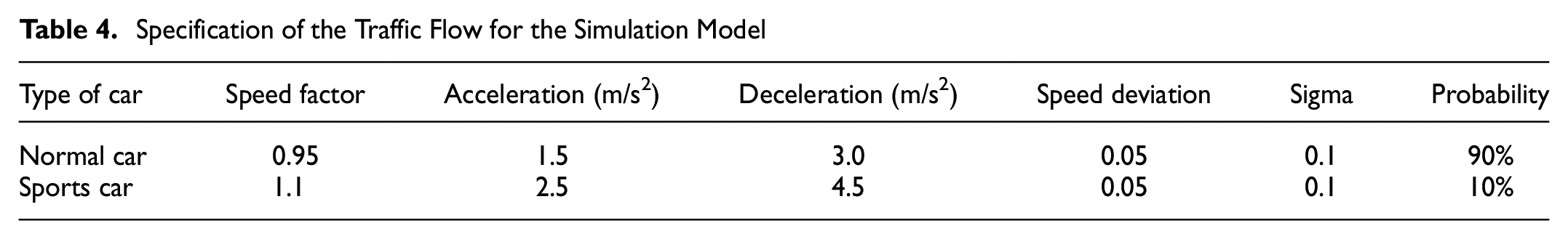
For evaluation of the results obtained from the mathematical optimization model, we use the microscopic traffic flow simulation tool SUMO (Version 1.4.0) ( 17 ). The traffic flow for the simulation model has been chosen at a probability of 18% for each of the two directions, that is, almost every 5 s there is a car entering the arterial at both of its ends, or about 16 cars per green phase (50 s) during one cycle (90 s) on average. The cars are chosen among two different types of cars, whose characteristics are displayed in Table 4.

Table 4.

Specification of the Traffic Flow for the Simulation Model

Type of car	Speed factor	Acceleration (m/s²)	Deceleration (m/s²)	Speed deviation	Sigma	Probability
Normal car	0.95	1.5	3.0	0.05	0.1	90%
Sports car	1.1	2.5	4.5	0.05	0.1	10%

To avoid isolated artifacts, for each optimization result, five simulation runs were performed with the following different random seeds: 301, 801, 903, 2,508, and 2,712, providing between 407 and 500 cars. Then, for each of the two directions separately, we can report the average number of stops of the cars, as well as the “time loss” ( 17 ) that the cars faced on average along the arterial, by having to drive slower than desired (cf. speed factor in Table 4), including waiting times. We refrain from reporting the values of each single run, because for each ID, the standard deviations turned out to be relatively small: at most 0.11 (ID17) for the number of stops and at most 6.91 (ID03) for the time loss. Instead, Table 5 reports the average number of stops per car and the average time loss per car separately for the two different directions. In more detail, for each case, five simulation runs were conducted with the five different random seeds. Within each such simulation run, the average number of stops and average time losses for each of the 407 to 500 cars was first computed. Finally, Table 5 reports for each case the average value of the aforementioned five average values.

Table 5.

Computational Results of the Simulation Model

ID	gd_j ,_yes	Sequence requirement	Green wave WE?	Solution quality for q=yes	Solution quality for q=no	Stops WE	Stops EW	Time loss WE	Time loss EW
00	–	c_j = 0, π_j,d,_GB = 0	no	(reference)		4.40	4.39	173	167
03	10	c_j = 0	no	200 (100%)	600 (60%)	4.70	3.67	185	147
07	10	c_j = 0	no	164 (82%)	660 (66%)	5.35	2.87	203	110
11	10	c_j ∈ {−1,0,+1}	yes	192 (96%)	794 (79%)	0.56	3.68	31	136
13	10	c_j ∈ {−1,0,+1}	no	192 (96%)	794 (79%)	1.36	3.23	62	123
15	10	c_j ∈ {−1,0,+1}	yes	172 (86%)	846 (85%)	0.55	3.29	30	120
17	10	c_j ∈ {−1,0,+1}	no	172 (86%)	846 (85%)	0.97	2.34	49	93
02	25	c_j = 0	yes	360 (72%)	660 (66%)	0.55	7.55	30	281
04	25	c_j = 0	no	488 (98%)	600 (60%)	3.80	4.69	144	181
08	25	c_j = 0	no	404 (81%)	660 (66%)	3.36	3.41	133	127
12	25	c_j ∈ {−1,0,+1}	yes	469 (94%)	794 (79%)	0.62	4.26	33	163
14	25	c_j ∈ {−1,0,+1}	no	492 (98%)	794 (79%)	2.28	2.57	91	109
16	25	c_j ∈ {−1,0,+1}	yes	442 (88%)	846 (85%)	0.57	3.26	31	119
18	25	c_j ∈ {−1,0,+1}	no	442 (88%)	846 (85%)	1.49	1.64	60	73

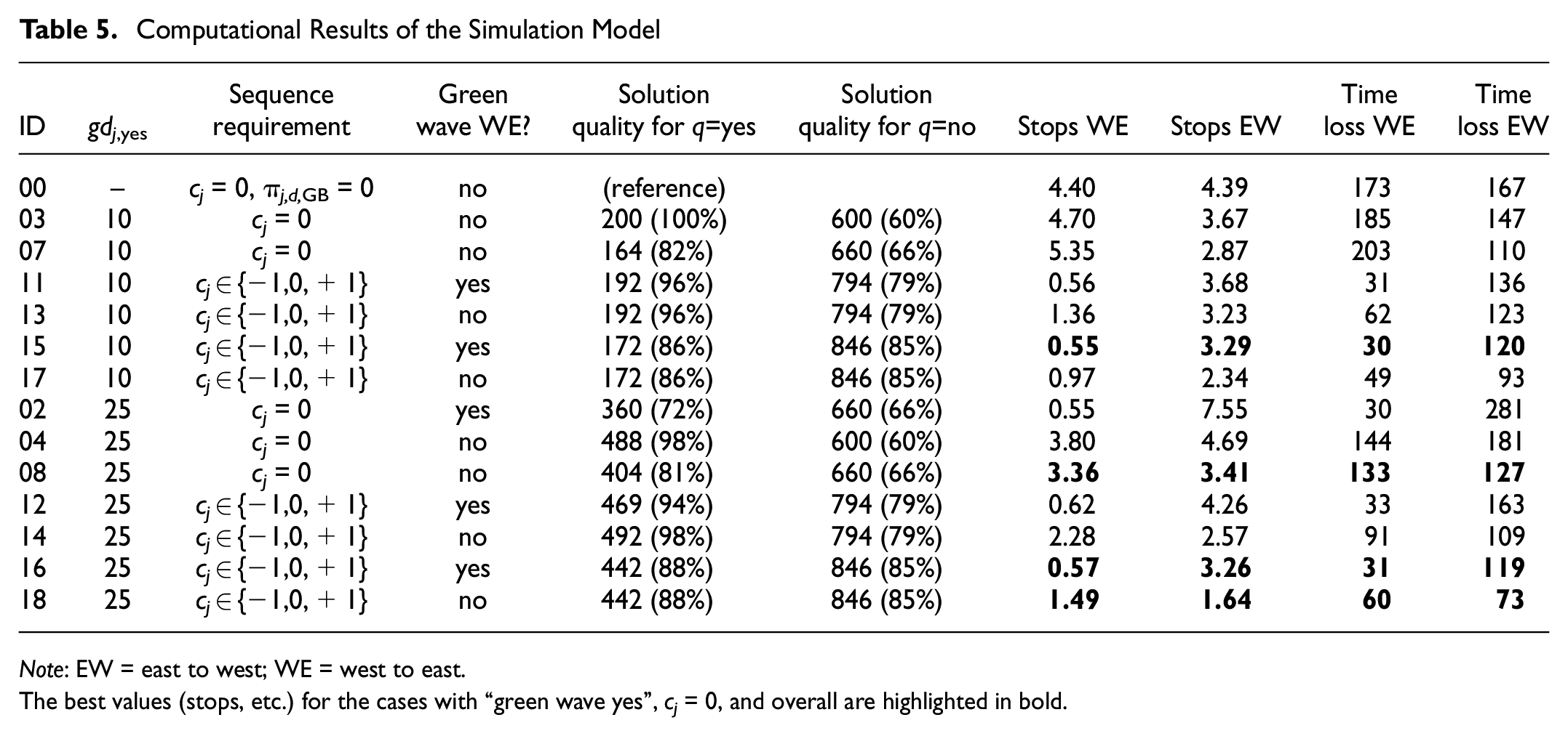
Note: EW = east to west; WE = west to east.

The best values (stops, etc.) for the cases with “green wave yes”, c_j = 0, and overall are highlighted in bold.

The best results have been obtained for ID18, in which

the left-turn phases may be arranged in an optimum way,

no green wave has to be established in one direction,

the portion of the green band that contributes with an extra weight to the objective function is 50% (i.e., 25 s of 50 s), and

within the objective function, priority is put on the entire green band (50 s) as a whole.

Recall that the values in Table 5 include the first junction, where the traffic flow is arriving uniformly at random. Therefore, one may expect already 40/90 = 0.44 stops there (red duration divided by the cycle time), amounting to expected average time losses of 20 s (half of the red duration). So, despite the explicitly unfavorable driving times between the junctions (cf. Table 2), coordination measures k larger than 88%—computing 1.64−0.44 = 1.2, (10−1.2)/10—have been achieved for both directions, while the green portion is just 55% (50 s/90 s) at each junction. According to the HBS ( 13 ), this is interpreted as “good quality.”

The two best cases with “green waves” are ID15 and ID16. The quality in this direction is of course “very good.” An expected number of stops of 0.13 = 0.57−0.44 and time loss of 11 s = 31 s−20 s could occur because, in the course of traveling along the arterial, platoons tend to spread out in the microscopic simulation because of the random distribution of their speeds. But the quality in the opposite direction is not even “medium,” but only “moderate,” because k = (10−2.82)/10 = 72%, where 2.82 = 3.26−0.44.

Finally, let us compare these cases in which the mathematical optimization model selected the phase sequences in an optimum way, with the best case in which at each junction both directions always have green at the same time. The best such case is ID08. The sum of the values of the average number of stops in both directions is more than twice as large as in the best case ID18—if we subtracted the expected number of stops at the first junction, the factor even amounts to as much as 2.6. With even more stops on average in both directions than in ID16 in the uncoordinated direction, the coordination quality is thus only “moderate” in both directions, somehow mirroring the explicitly unfavorable driving times between the junctions (cf. Table 2). Interestingly enough, this optimized result (ID08) does only show a small improvement over the totally uncoordinated reference case ID00, in which at each junction the green phases in both directions simply start at time zero.

We conclude the presentation of the computational results by illustrating the green bands of the two cases ID08 in Figure 8 and ID18 in Figure 9 in time–space diagrams.

Figure 8.

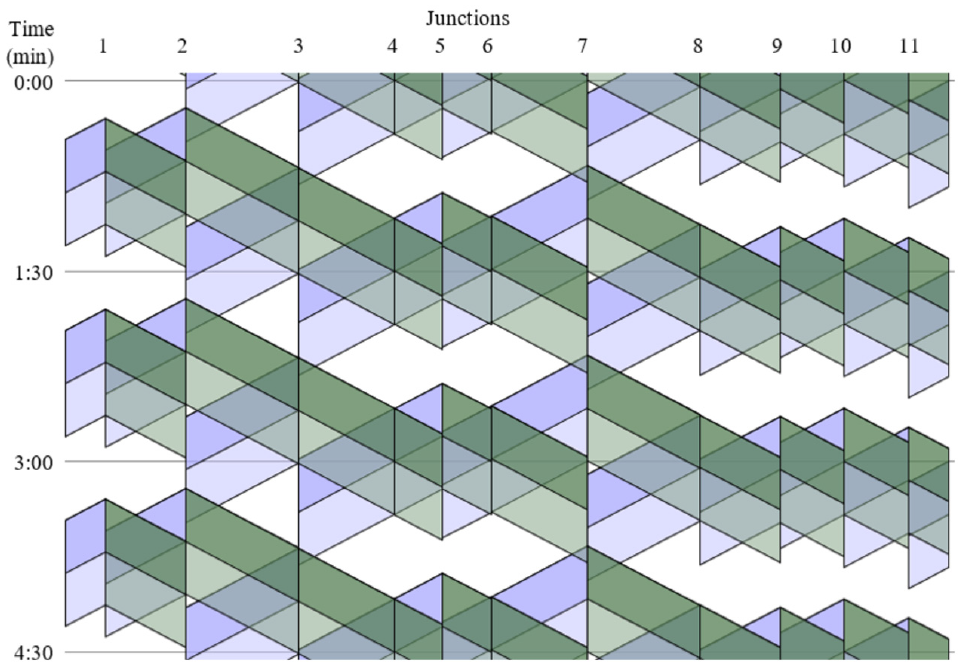
Illustration of the green bands in both directions for the best scenario, ID08, in a time–space diagram. The first 25 s of the green bands are displayed as solid, while the last 25 s of the green bands are displayed as more transparent. At all junctions j, both directions are always green at the same time (i.e., c_j = 0).

Figure 9.

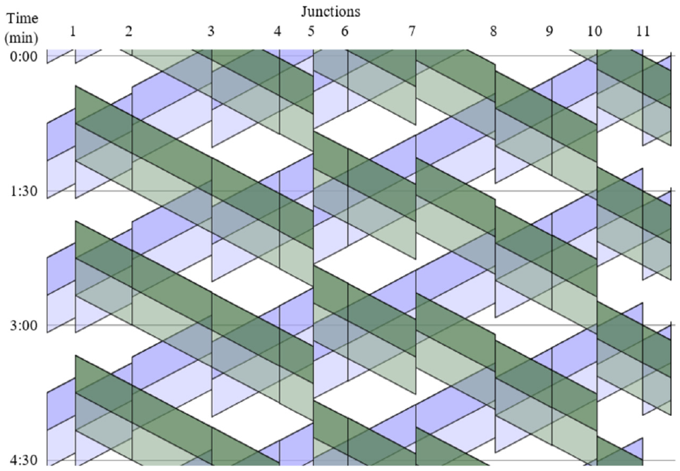
Illustration of the green bands in both directions for ID18 in a time–space diagram. The first 25 s of the green bands are displayed as solid, while the last 25 s of the green bands are displayed as more transparent. In the optimization result, there is no junction j at which both directions are green at the same time (i.e., c_j = 0).

Please refer to the appendix to see the time–space diagrams of two IDs with green waves in the WE direction (ID02 and ID16): the former with identical green phases for both directions, the latter with adjusted left-turn phases for the two directions independently from each other. Finally, let us also increase the traffic volume. To this end, we evaluate ID18 with a traffic flow probability of 50%, instead of only 18% as was applied in Table 5. Here, it might be worth recalling that the green portion is 55%. The number of expected stops per direction increases only slightly, by no more than 0.3, to 1.79 and 1.91. Similarly, the average time loss increases by only 15 s and 18 s, to 76 s and 90 s, respectively (random seed 2,712, 1,180 cars). The interested reader may continue to work with this publicly available data set ( 18 ).

Conclusion

The paper proposes a PESP-based integer linear optimization model that adds decisions of phase sequencing, partly even phase selection, to the task of coordinating the offsets between fixed-time traffic light programs. This model is applied to an artificial arterial road with 11 junctions. The computational results provide clear evidence for the benefit of including decisions of phase sequencing (phase selection). In the data set, first, immediately in the optimization model, the solution quality for the parts of all arriving platoons which may pass the next junction without any stop increases from 66% to 85% (cf. IDs 02, 07, and 08 versus 15–18).

Moreover, second, this improvement is also reflected in the detailed evaluation in a microscopic traffic flow simulation. There, compared with offsets that are optimal with respect to the objective function, the best case with a dedicated selection of the actual phases and their sequences reduced the average number of stops from 3.36 (WE) and 3.41 (EW) to 1.49 (WE) and 1.64 (EW), that is, a reduction by more than 53%. It would be of interest to compare the results on the used data set ( 18 ) with results achieved by the (commercial) software that is frequently applied in practice, such as LISA, Synchro or TRANSYT ( 5 ).

In particular, when comparing the somewhat local objective function (Equation 11) in this case with the actual coordination measure according to the HBS ( 13 ), one relevant potential line of improvement becomes obvious. That is to turn the local nature of our objective function into one that follows the green band over more than just the immediately next junction, that is, along (small) paths rather than just edges.

Supplemental Material

sj-docx-1-trr-10.1177_03611981231170129 – Supplemental material for Bidirectional Green Waves for Road Arterials: Optimization and Simulation

Supplemental material, sj-docx-1-trr-10.1177_03611981231170129 for Bidirectional Green Waves for Road Arterials: Optimization and Simulation by Christian Liebchen in Transportation Research Record

Footnotes

Acknowledgements

The author thanks Berenike Masing and Niels Lindner for a fruitful discussion in the early stages of the development of the optimization model, in particular its objective function. In addition, the author thanks Bernhard Friedrich, Klaus Nökel, and Peter Wagner for worthwhile comments.

Author Contributions

The author confirms sole responsibility for the following: study conception and design, data collection, analysis and interpretation of results, and manuscript preparation.

Declaration of Conflicting Interests

The author declared no potential conflicts of interest with respect to the research, authorship, and/or publication of this article.

Funding

The author received no financial support for the research, authorship, and/or publication of this article.

ORCID iD

Christian Liebchen

Supplemental Material

Supplemental material for this paper is available online.

References

Foresite Group. A Beginners’ Guide to Traffic Signal Timing. 2021. https://www.foresitegroup.net/post/a-beginner-s-guide-to-traffic-signal-timing/. Accessed April 28, 2023.

Serafini

Ukovich

A Mathematical Model for Periodic Scheduling Problems. SIAM Journal on Discrete Mathematics, Vol. 2, No. 4, 1989, pp. 550–581.

Hassin

A Flow Algorithm for Network Synchronization. Operations Research, Vol. 44, No. 4, 1996, pp. 570–579.

Wünsch

Coordination of Traffic Signals in Networks. PhD thesis, Technical University Berlin, Germany, 2008.

Binning

J. C

. TRANSYT 16 User Guide. TRL Ltd., Crowthorne, 2010.

Gartner

N. H.

Assmann

S. F.

Lasaga

Hou

D. L.

A Multi-Band Approach to Arterial Traffic Signal Optimization. Transportation Research Part B: Methodological, Vol. 25, No. 1, 1991, pp. 55–74.

Zhang

Yuanchang

Gartner

N. H.

Stamatiadis

Arsava

AM-Band: An Asymmetrical Multi-Band Model for Arterial Traffic Signal Coordination. Transportation Research Part C: Emerging Technologies, Vol. 58, 2015, pp. 515–531.

Jing

Lin

Shou

Pband: A General Signal Progression Model With Phase Optimization Along Urban Arterial. IEEE Transactions on Intelligent Transportation Systems, Vol. 23, No. 1, 2022, pp. 344–354.

Köhler

Strehler

Traffic Signal Optimization Using Cyclically Expanded Networks. Networks, Vol. 65, No. 3, 2015, pp. 244–261.

10.

Köhler

Strehler

Traffic Signal Optimization: Combining Static and Dynamic Models. Transportation Science, Vol. 53, No. 1, 2019, pp. 21–41.

11.

Liebchen

Maximizing Bidirectional Green Waves for Major Road Axes. Preprint. Technische Hochschule Wildau, Germany, 2021. https://doi.org/10.15771/2827.

12.

Eom

Kim

B.-I.

The Traffic Signal Control Problem for Intersections: A Review. European Transport Research Review, Vol. 12, 2020, pp. 1–20.

13.

Forschungsgesellschaft für Straßen- und Verkehrswesen (FGSV). Handbuch für die Bemessung von Straßenverkehrsanlagen (HBS) – Teil S: Stadtstraßen. FGSV-Verlag GmbH, Köln, 299, 2015 (in German).

14.

Chapter 6, Coordination. Traffic Signal Timing Manual. U.S. Department of Transportation, Federal Highway Administration, 2021. https://ops.fhwa.dot.gov/publications/fhwahop08024/chapter6.htm. Accessed October 5, 2021.

15.

Liebchen

Periodic Timetable Optimization in Public Transport. PhD dissertation. Verlag im Internet, Technische Universität, Berlin, Germany, 2006.

16.

Lindner

Liebchen

Determining All Integer Vertices of the PESP Polytope by Flipping Arcs. In Proc., ATMOS 2020 ( Huisman

Zaroliagis

, eds.), OASIcs, 2022, Schloss Dagstuhl - LeibnizZentrum für Informatik, Germany, Vol. 85, pp. 5:1–5:18.

17.

Deutsches Zentrum für Luft- und Raumfahrt (DLR). SUMO – Simulation of Urban Mobility. 2022. https://www.eclipse.org/sumo/. Accessed July 18, 2022.

18.

Liebchen

Bidirectional Road Arterial - Traffic Signal Optimization - 11 Junctions. Mendeley Data, Version 1, 2023. http://dx.doi.org/10.17632/928hch53cp.1.

Supplementary Material

Please find the following supplemental material available below.

For Open Access articles published under a Creative Commons License, all supplemental material carries the same license as the article it is associated with.

For non-Open Access articles published, all supplemental material carries a non-exclusive license, and permission requests for re-use of supplemental material or any part of supplemental material shall be sent directly to the copyright owner as specified in the copyright notice associated with the article.

0.00 MB

0.21 MB

From/to	2	3	4	5	6	7	8	9	10	11
1	20	48	72	84	96	120	148	168	184	200
2	-	28	52	64	76	100	128	148	164	180
3	-	-	24	36	48	72	100	120	136	152
4	-	-	-	12	24	48	76	96	112	128
5	-	-	-	-	12	36	64	84	100	116
6	-	-	-	-	-	24	52	72	88	104
7	-	-	-	-	-	-	28	48	64	80
8	-	-	-	-	-	-	-	20	36	52
9	-	-	-	-	-	-	-	-	16	32
10	-	-	-	-	-	-	–		-	16

From/to	2	3	4	5	6	7	8	9	10	11
1	20	48	72	84	96	120	148	168	184	200
2	-	28	52	64	76	100	128	148	164	180
3	-	-	24	36	48	72	100	120	136	152
4	-	-	-	12	24	48	76	96	112	128
5	-	-	-	-	12	36	64	84	100	116
6	-	-	-	-	-	24	52	72	88	104
7	-	-	-	-	-	-	28	48	64	80
8	-	-	-	-	-	-	-	20	36	52
9	-	-	-	-	-	-	-	-	16	32
10	-	-	-	-	-	-	–		-	16

From/to	2	3	4	5	6	7	8	9	10	11
1	20	48	72	84	96	120	148	168	184	200
2	-	28	52	64	76	100	128	148	164	180
3	-	-	24	36	48	72	100	120	136	152
4	-	-	-	12	24	48	76	96	112	128
5	-	-	-	-	12	36	64	84	100	116
6	-	-	-	-	-	24	52	72	88	104
7	-	-	-	-	-	-	28	48	64	80
8	-	-	-	-	-	-	-	20	36	52
9	-	-	-	-	-	-	-	-	16	32
10	-	-	-	-	-	-	–		-	16