Sage Journals: Discover world-class research

Abstract

Assessing sulfate concentration levels and their distributions within road alignments is crucial for the design of highway projects. Sulfate minerals in soils react with calcium-based additives, leading to sulfate-induced heaving and pavement failures. However, a reasonable assessment of the extent and levels of sulfate concentration using current practices, such as conventional laboratory-based methods, is still challenging because of the spatial heterogeneity of sulfate minerals and their seasonal fluctuations. This study aims to assess the application of electrical resistivity imaging (ERI) to determine levels and distributions of sulfate concentration. Finite element and least-squares optimization were used to process the data and generate subsurface inverted resistivity profiles. Fourteen ERI surveys were carried out for two sites with a potentially high risk of sulfate-induced heaving to help determine the extent of critical sulfate concentration zones. Laboratory tests (sulfate and moisture content tests) were conducted on ten samples collected from the field sites to validate ERI findings. The results showed that electrical resistivities of critical sulfate concentration zones are significantly lower than typical ranges of electrical resistivity of earth materials because of the abundance of salt ions in pore water, which facilitates the flow of electric current. The findings of this study were consistent with laboratory test results in determining the sulfate concentration levels. This study showed that ERI successfully provides a rapid and continuous assessment of critical sulfate concentration zones within highway alignments. The findings of this study will help materials and pavement engineers determine where alternative materials and pavement designs are needed.

Keywords

infrastructure stability electrical resistivity imaging sulfate concentration risk of sulfate-induced heaving subsurface exploration

Heaving and premature failure of pavements constructed on stabilized soils are primarily caused by the reaction of calcium-based stabilizers with sulfate-rich soils. Calcium-based stabilizers react with sulfate and clay minerals, specifically montmorillonite, in the presence of water and form new expansive minerals such as ettringite ( 1 , 2 ). Hydration of these minerals or growth of the crystalline minerals leads to the failure of pavements known as “sulfate-induced heaving.” In the United States, more than fifteen state Departments of Transportation (DOTs) deal with pavement failures associated with sulfate-induced heaving, resulting in high maintenance costs and safety concerns ( 3 ). The repairing cost of such pavements is in the order of millions of dollars and exceeds the cost of soil stabilization ( 4 – 6 ). Road maintenance activities consume a large share of state transportation budgets, which are limited to the maintenance of different assets of transportation agencies ( 7 – 12 ). Extensive research has been conducted to associate the risk of sulfate-induced heaving with sulfate concentration levels. For example, the Texas Department of Transportation (TxDOT) has guidelines for stabilizing sulfate-rich soils and associates a low risk of sulfate-induced heaving in soils with sulfate concentrations below 3,000 ppm ( 13 ). Conversely, the potential risk of sulfate-induced heaving is high in soils with sulfate concentrations above 8,000 ppm. There is a moderate risk of sulfate-induced heaving in soils with sulfate concentrations between 3,000 and 8,000 ppm. Identifying the risk of sulfate-induced heaving (i.e., determining the sulfate concentration levels) before soil investigation is crucial to help develop effective site exploration and sampling techniques, define sampling and testing intervals, and specify required controls during construction ( 14 ).

Sulfate concentration in soils is commonly measured by conventional laboratory-based methods such as chromatography, colorimetry, and gravimetry. For areas with potentially high sulfate concentrations, a minimum frequency of every 152 m (500 ft) along the roads is recommended between the sampling locations ( 13 ). The conventional methods of sulfate testing provide accurate measurements of sulfate concentration; however, this information is point specific and sparse. In other words, these methods do not yield a continuous assessment of sulfate concentrations and could miss a critical sulfate concentration zone if it lies between the sampling locations.

Another way to identify areas with a potentially high risk of sulfate-induced heaving is through web-based maps. One of the largest natural resource information systems is the Web Soil Survey (WSS), operated by the United States Department of Agriculture. Although the WSS provides information about the gypsum content and soil salinization risk for different geologic regions, this information has a high level of detail and lacks enough resolution ( 15 ). In addition, this information might not be accurate, as sulfate concentrations in soils are subject to seasonal fluctuations ( 13 ). Other maps that show soil mineralogy and subsurface formations (e.g., maps from the Bureau of Economic Geology) also suffer from the limitations of the WSS map ( 15 ).

A few researchers have used an electrical conductivity mapping system to develop prediction models for determining sulfate concentration based on soil electrical conductivity (i.e., reciprocal of soil electrical resistivity). They utilized the Veris 3150 system, commonly used for agriculture applications, to collect electrical conductivity values in three different fields. This system is equipped with multiple heavy-duty Coulter electrodes that are attached to a disk harrower. The Veris 3150 system measures the soil electrical conductivity as the disks cut through the soil. Harris et al. collected electrical conductivity data from field sites using the Veris 3150 system and measured the sulfate concentrations for specific locations ( 15 ). They analyzed the obtained data by linear regressions and found that the sulfate concentration has a direct non-linear relationship with soil electrical conductivity ( 15 ). They used a natural logarithm to transform the sulfate concentration values and developed a regression based on electrical conductivities. Shon et al. ( 16 ) replicated Harris et al.’s ( 15 ) approach and used a linear regression model for generating color-coded maps for sulfate concentrations in specific areas. There are some challenges and limitations to these studies. The developed linear regressions might lead to misleading results as they cannot handle non-linear relationships between response and predictor variables, which is evident between electrical conductivity and sulfate concentration ( 17 – 19 ). In addition, the electrical conductivity mapping system cannot provide continuous measurements throughout the depth and only collects the data at two depths of 0.3 m and 1 m (1 and 3 ft) ( 20 ). The maximum penetration depth of the electrical conductivity mapping system is 1 m, which provides inadequate information for assessing the subsurface conditions for pavement designs (at least 2 m is required) ( 21 ). Moreover, the system cannot be employed along the highway’s rights-of-way, and its applicability highly depends on the site accessibilities because of the large dimensions of the system.

Recently, instead of determining the sulfate concentration levels, Puppala studied the heaving potential of cement- and lime-stabilized soils in a field to help evaluate practical methods for treating sulfate-rich soils ( 3 ). He developed a hybrid sensor and found that the risk of sulfate-induced heaving can be identified by the loss of soil stiffness (small-strain shear modulus). The loss of soil stiffness is higher in cement-stabilized than lime-stabilized soils ( 3 ). Despite the importance of this study, it has some challenges and problems. First, it cannot provide continuous information about the soil heaving potential. The hybrid sensor must be embedded in soil at 20 cm (8 in.) deep to monitor the water content and soil stiffness at different periods ( 3 ). Second, sufficient water content should be supplied continuously during the experiment to stimulate chemical reactions; insufficient water content results in inaccurate interpretations of the soil heaving potential. Third, the hybrid sensor is subject to tear and wear because of the movement of vehicles. Last, the experiment is time-consuming and requires monitoring and collection of data for about 10–30 days ( 3 ).

In summary, a reasonable assessment of the extent and levels of sulfate concentration using the current practices, such as laboratory-based methods, is challenging for two main reasons: (1) sulfate minerals are not uniformly distributed along the roads, and the current methods might miss a high sulfate concentration zone because of the lack of information between the measurements ( 14 , 15 ), and (2) sulfate concentrations in soil are highly variable because of variations in precipitation and seasonal fluctuations in the groundwater table which result in uncertainty to the risk level associated with chemical stabilization ( 14 , 22 ). This study aims to assess the application of electrical resistivity imaging (ERI) to determine the levels and distributions of sulfate concentration for specific sites. Federal Highway Administration (FHWA) recommends ERI as one of the geophysical methods for improving site characterization and maximizing return-on-investment ( 18 ). The ERI is a powerful tool to evaluate subsoil heterogeneity and provide fill-in data between the boreholes through a cost-effective and rapid approach ( 18 ). Therefore, a complete assessment of subsurface conditions can be accomplished by combining geotechnical and electrical resistivity data. However, like all other geophysical methods, the ERI method provides non-unique results and the findings from surveys are specific to the geology and site conditions. The proposed approach in this paper is expected to assist the state DOTs in determining highway segments that are unlikely to suffer from sulfate-induced heaving and identify areas that may contain critical concentrations of sulfate.

Study Approach

Study Sites

Two case studies with a potentially high risk of sulfate-induced heaving in the north-central part of the U.S. state of Texas were selected to be the focus of this research (Figure 1). Site 1 is situated in a region mapped with Eagle Ford formation and is bound by a lake to the west. The Eagle Ford formation consists of shale, siltstone, and limestone, and has an estimated thickness of 90–120 m (300–400 ft) in north Texas. Geotechnical analysis (from September 2021) from two boreholes indicates that the existing asphalt pavements consist of a dense crushed limestone layer (<1 m depth) at the surface. Directly beneath the limestone layer, stiff to hard, fat (CH) and lean (CL) clays are extended to a depth of 6 m (20 ft). The sulfate concentration at the top layer was measured in the range of 20 to 22,080 ppm. Dry-auger drilling technique was used for the two borings, allowing short-term groundwater observations. Groundwater was not observed in any soil test borings at Site 1 during drilling.

Figure 1.

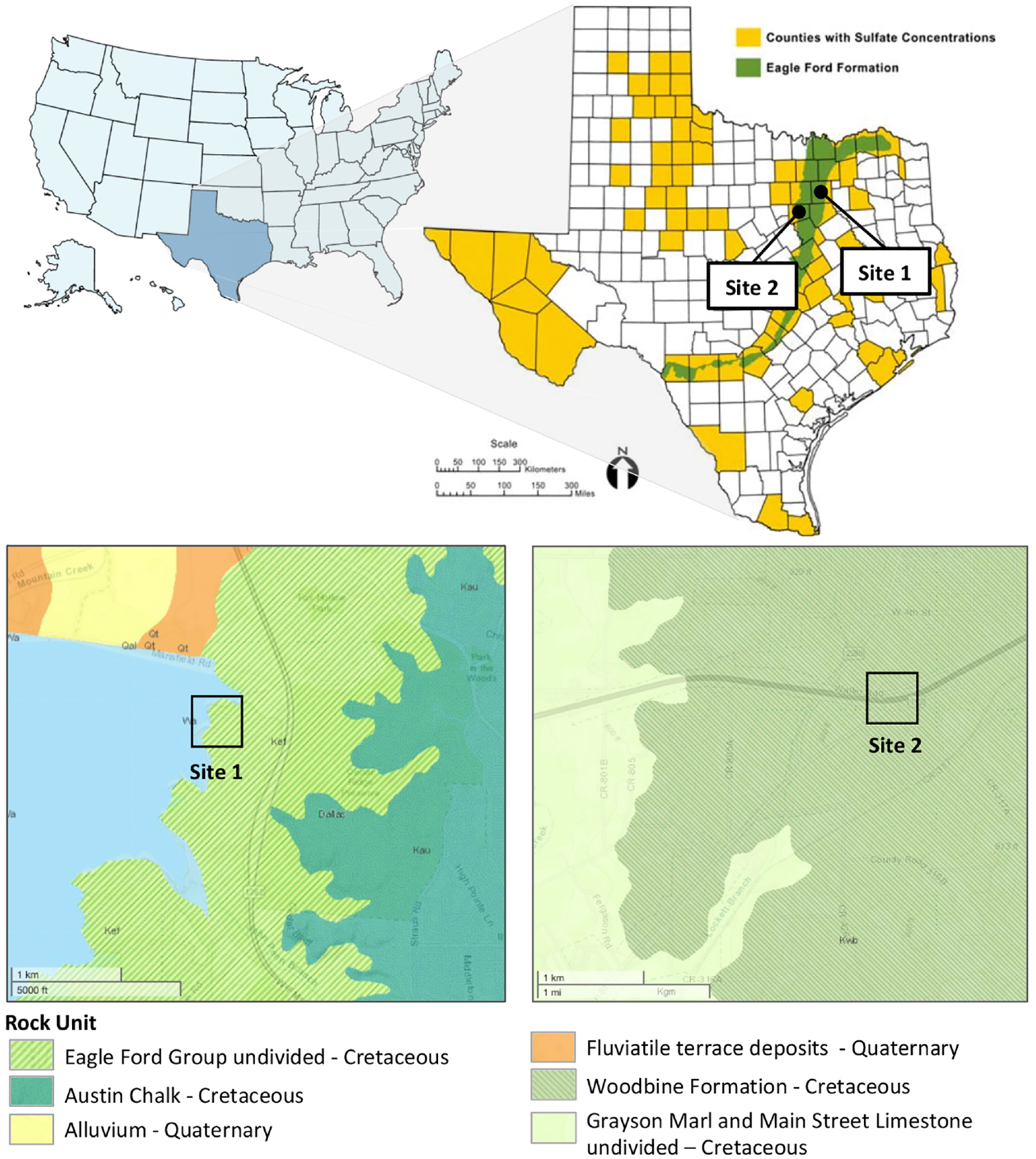
Location of the case studies on the map of Texas and the geologic maps.

Site 2 is situated in a region mapped with the Woodbine formation. The Woodbine formation consists primarily of sandstone and shale with a thickness of about 100 m (320 ft). Geotechnical analysis (from December 2020) from three boreholes indicates complex geology at this site, consisting of fat (CH) and lean (CL) clays underlain by clayey sand (SC) at some locations. The depth of the clayey sand layer varies from 0.3 to 3 m (1 to 9 ft). In some areas, there is a dense layer (shale) at a minimum of 3 m (9 ft) deep. The observations of sulfate concentration at Site 2 were higher than at Site 1 and ranged from 82 to more than 40,000 ppm. During dry-auger drilling, a trace of water was observed at a minimum of 3 m (10 ft) at two of the soil borings at Site 2.

Because of the observed high sulfate concentrations, these study sites required further investigation to help determine appropriate methods for stabilizing the soil.

Data Collection

Electrical Resistivity Imaging

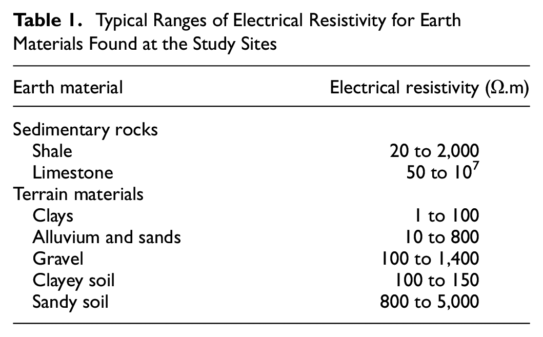
ERI is one of the suggested geophysical methods by FHWA that complements conventional geotechnical site investigations to provide fill-in information about the characteristics and heterogeneities of subsurface materials ( 18 ). The electrical resistivity of the subsurface is measured by inducing an electrical current into the ground across two electrodes and receiving the resulting voltage from the other two electrodes. In practice, many electrodes (e.g., twenty-eight, fifty-six, or more) and multi-electrode cables are used to speed up the data acquisition and improve the quality of large datasets ( 23 ). Simultaneous measurements can be recorded using a multi-electrode array; a switching box automatically selects and switches the relevant four electrodes based on the predefined sequence (defined in a command file) stored in the resistivity meter ( 24 ). A continuous subsurface pseudo-section is then generated using the measured apparent electrical resistivities. For plotting the pseudo-sections from the 2D data, electrical resistivity measurements are displayed at the intersection of two 45° lines starting from the center of the current and potential electrode pairs ( 25 ). Table 1 lists typical ranges of electrical resistivity for earth materials found at the study sites. The soil and rock matrix, the percentage of fluid saturation, and the conductivity of pore fluids (which is proportional to the concentration of salt ions such as sulfate) mainly influence the electrical properties of earth materials (26 –28).

Table 1.

Typical Ranges of Electrical Resistivity for Earth Materials Found at the Study Sites

Earth material	Electrical resistivity (Ω.m)
Sedimentary rocks
Shale	20 to 2,000
Limestone	50 to 10⁷
Terrain materials
Clays	1 to 100
Alluvium and sands	10 to 800
Gravel	100 to 1,400
Clayey soil	100 to 150
Sandy soil	800 to 5,000

Fourteen 2D ERI surveys were conducted using different electrode spacings to investigate the extent of high sulfate concentration zones at the study sites. The arrangement of ERI lines is illustrated in Figure 2. The ERI lines were conducted on top of the borings performed by the dry-auger drilling technique at Site 2. However, as the surface is paved at Site 1, the unpaved sections at the closest distances to the borehole locations were selected to perform the ERI lines, where there was enough space to spread the electrodes and lay out the resistivity lines. Electrodes’ contact resistance with the soil was below a threshold level of 2,000 ohm for all ERI lines ( 29 ).

Figure 2.

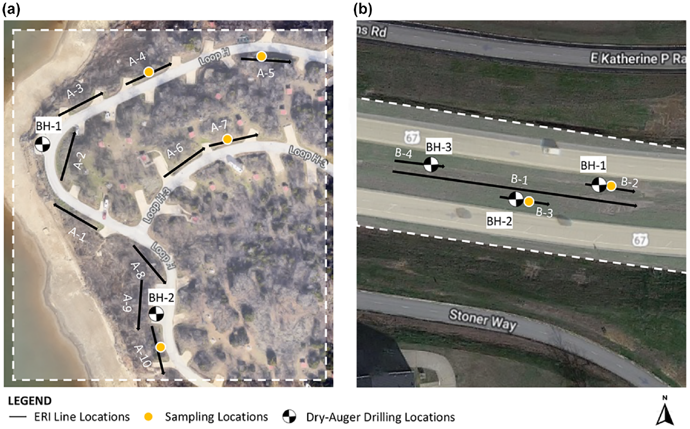
Arrangement of ERI lines and sampling locations: (a) Site 1 and (b) Site 2.

The electrical resistivity measurements were conducted using the AGI SuperSting R8/IP instrument, multi-electrode cables, and stainless-steel electrodes. The electrode spacings were determined based on the desired penetration depth and sites’ accessibility, ranging from 0.6 and 2.4 m (2 ft and 8 ft). The electrodes were installed into the ground at equal distances, and a dipole-dipole array was employed to explore the subsurface conditions. The apparent electrical resistivity value is calculated by Equation 1 using the dipole-dipole array.

ρ_{a} = π n (n + 1) (n + 2) a \frac{Δ V}{I}

(1)

where n is a factor ranging from 1 to 6, a is the electrode spacing, ΔV is the voltage drop, and I is the electrical current. The sensitivity of the dipole-dipole array to the horizontal variations is more than the vertical variations ( 25 ). The dipole-dipole array can provide detailed information at shallow depths ( 30 ). It can therefore better delineate the subsurface anomalies, such as critical sulfate concentration zones, than other electrode configurations. Moreover, forward modeling was carried out to further examine the capability of various electrode configurations in delineating horizontal anomalies such as a high sulfate concentration zone. Figure 3 shows a synthetic resistivity model with two conductive blocks (representing different zones of high moisture and sulfate concentration) embedded in a low resistive medium (representing moist clayey soil). The model was constructed using twenty-eight electrodes spaced every 0.6 m (2 ft) to be consistent with the majority of the conducted ERI lines.

Figure 3.

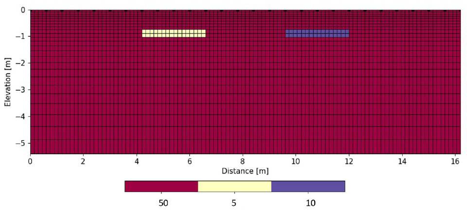
Synthetic resistivity model with two conductive blocks embedded within a low resistive area.

Figure 4 shows the inversion results obtained by forward modeling for the synthetic model using four built-in electrode configurations in ResIPy software (dipole-dipole, Wenner, Schlumberger, multi-Gradient) and 2% noise in the data. Each model inversion was completed within five iterations with a root mean square error of less than 1.2%. According to Figure 4, each of the four electrode configurations can reconstruct the two conductive blocks of the synthetic model to a certain degree. The conductive zones are at least twice the thickness of the known blocks (0.3 m) in all models reconstructed. The Schlumberger and multi-Gradient arrays reconstructed more vertical than horizontal shapes, which is inconsistent with the shape of known blocks. However, the dipole-dipole and Wenner arrays show more consistent reconstructed shapes and produced less heterogeneity than the other two arrays. Although dipole-dipole and Wenner represent similar reconstructed models, a major difference between them is the thickness of the transition zones within the conductive blocks and the background in the horizontal direction. The dipole-dipole array better defines the horizontal extent of the conductive blocks at the correct depth. Besides, the reconstructed model based on the dipole-dipole array shows a more consistent medium at the shallow subsurface with less heterogeneity compared with the reconstructed models based on the Wenner array.

Figure 4.

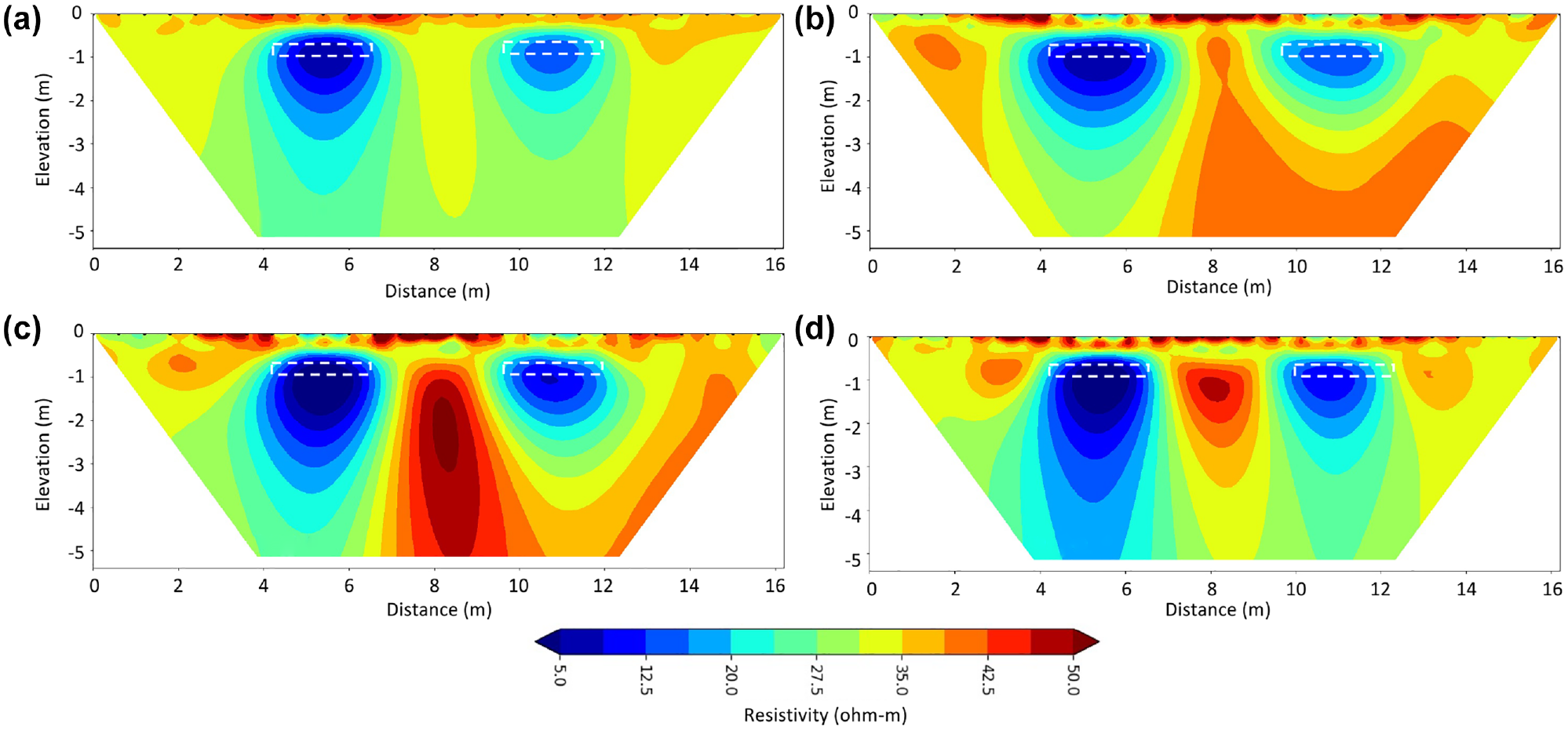
Inversion results for synthetic resistivity model based on four array configurations: (a) dipole-dipole, (b) Wenner, (c) Schlumberger, and (d) multi-gradient.

Furthermore, forward modeling was carried out based on a synthetic model shown in Figure 5 to illustrate how a saltwater saturated zone (high sulfate concentration zone) can be differentiated from freshwater saturated clays. These blocks are overlaid by a more resistive block at the top. Figure 5b shows the inversion results of the synthetic model using a dipole-dipole array. According to Figure 5b, a low electrical resistivity anomaly distinguishes the zone of high sulfate concentration (conductive block) which is centered at 8 ft distance. Although the reconstructed model does not match the actual depth of the conductive block, it accurately represents the extent of the conductive block that is of interest in determining zones with potential sulfate-induced heaving.

Figure 5.

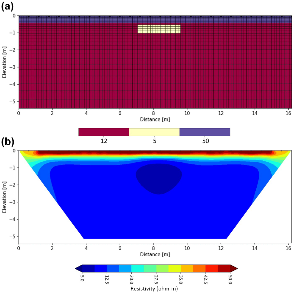
Forward modeling of: (a) synthetic model with three blocks and (b) inversion results using a dipole-dipole array.

Laboratory Testing

To later validate the ERI findings, ten soil samples were collected from the shallow subsurface (the top 0.6 m) along the ERI lines. The locations of the collected samples are also shown in Figure 2. Table 2 presents the laboratory test results for the soil samples associated with ERI lines. The sulfate concentration of the soil samples was determined using a colorimetric method based on TxDOT 145-E. The moisture contents of the soil samples were also measured following ASTM D2216-90.

Table 2.

Summary of Laboratory Test Results

ERI line	Sample	Depth in m (ft)^a	Moisture content (%)	Sulfate concentration from sampling (ppm)	Sulfate concentration from dry-auger drilling (ppm)
A-2	BH-1	0.4 (1–1.5)	NA	NA	22,080
A-4	S1	0.2 (0–1.0)	14.4	Below 250	NA
A-5	S2	0.3 (0.5–1.5)	23.3	13,650	NA
	S3	0.6 (1.5–2.5)	28.7	33,550	NA
A-7	S4	0.2 (0–1.0)	14.5	Below 250	NA
A-9	BH-2	0.4 (1–1.5)	NA	NA	17,835
A-10	S5	0.3 (0.5–1.5)	14.8	4,500	NA
	S6	0.5 (1.0–2.0)	16.6	3,000	NA
B-2	S7	0.4 (1.0–1.5)	25.9	3,800	NA
	S8	0.6 (1.5–2.5)	29.7	17,000	19,200
	BH-1	1.2 (3–4)	NA	NA	40,000
B-3	S9	0.4 (1.0–1.5)	28.3	550	NA
	S10	0.6 (1.5–2.5)	30.1	1,250	667
	BH-2	1.2 (3–4)	NA	NA	21,378
B-4	BH-3	0.4 (1.0–1.5)	NA	NA	780
	BH-3	1.2 (3–4)	NA	NA	300

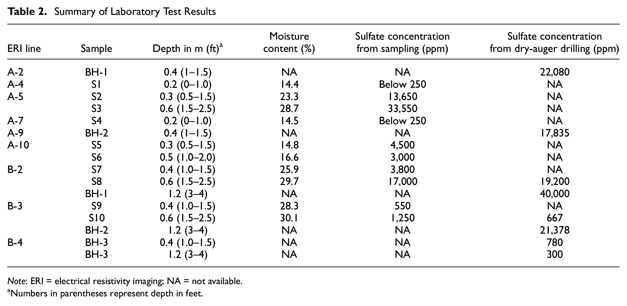
Note: ERI = electrical resistivity imaging; NA = not available.

Numbers in parentheses represent depth in feet.

Data Processing

The measured apparent resistivities were inverted using the EarthImager program to generate subsurface resistivity profiles. Figure 6 shows a typical flowchart of electrical resistivity data processing.

Figure 6.

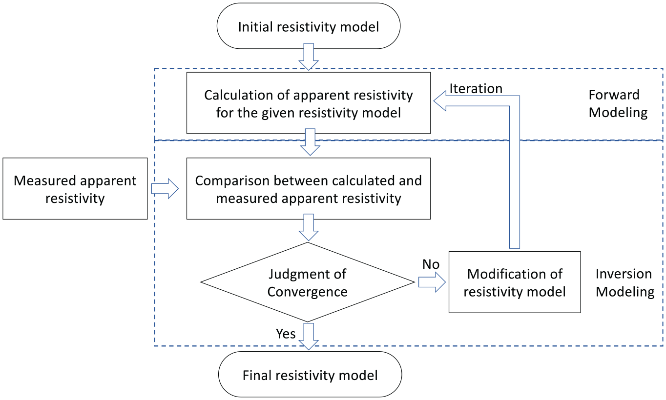
Typical flowchart of data processing.

In forward modeling, apparent resistivities are calculated using the resistance measurements and the geometric factor of the electrode configuration (Equation 1). The subsurface area is divided into many rectangular cells using a finite element method, and theoretical apparent resistivities are calculated based on Poisson’s equation for each block under certain conditions ( 32 , 33 ). Half the distance between electrodes was selected as the width of each cell ( 34 ). The mesh was then transformed based on the elevation data obtained from Google Earth to reflect the surface topography into the inverted resistivity profiles. In inversion modeling, the true apparent resistivities for each cell were predicted using a non-linear least-square optimization method, while reducing the misfit values between the predicted and measured apparent resistivities ( 25 , 35 ). The error difference between the measured and predicted models is evaluated by the root mean squared (RMS) error and is defined by Equation 2.

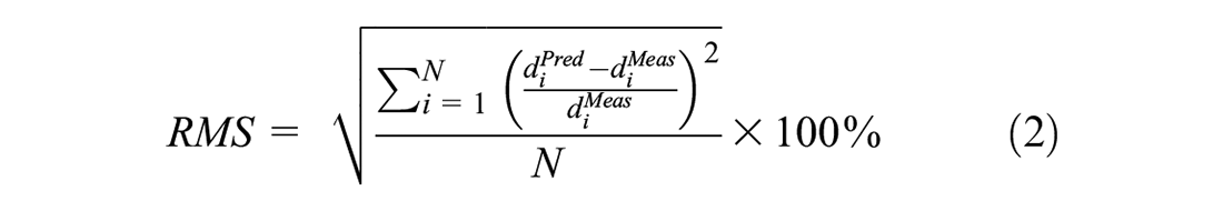
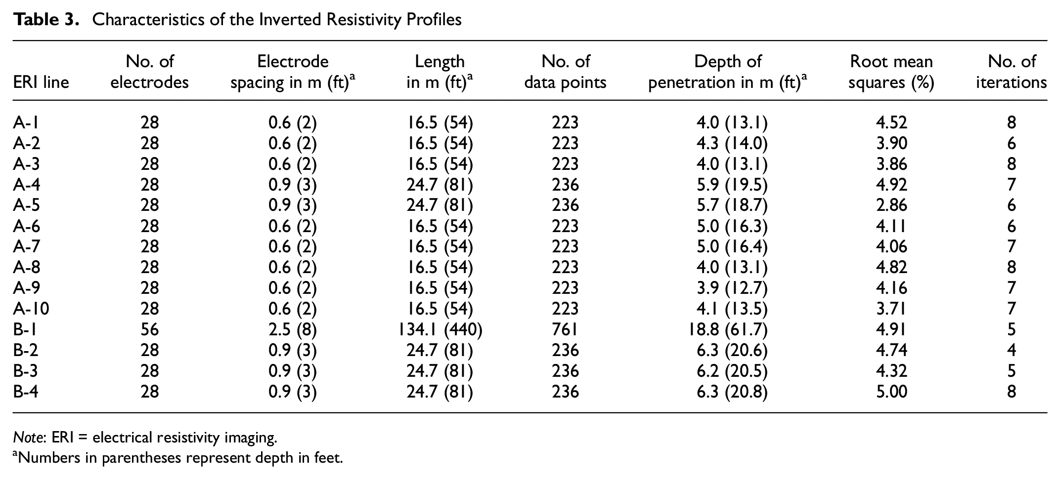
R M S = \sqrt{\frac{\sum_{i = 1}^{N} {(\frac{d_{i}^{P r e d} - d_{i}^{M e a s}}{d_{i}^{M e a s}})}^{2}}{N}} \times 100 %

(2)

where N is the number of measurements, d^Pred is the predicted apparent resistivity, and d^Meas is the measured apparent resistivity. RMS threshold of 5% was considered a stopping criterion through the inversion process ( 29 , 36 ), which was satisfied after four to eight iterations for most of the ERI lines. However, the error convergence was not achieved after several iterations for a few datasets because of noisy readings. Therefore, the poorly fit data were removed in a few steps, and the inversion process was repeated after each step to obtain the best model fit. Table 3 shows the main characteristics of the inverted resistivity profiles for study sites. Some factors were selected based on the data quality while generating the inverted resistivity sections to avoid much artifact development. For example, the starting model for inversion plays a critical role in data processing; an interpolated pseudo-section was adapted as the starting model for the clean resistivity data. Also, to ensure that the obtained resistivity profiles are consistent with the subsurface conditions, the resistivity profiles were regenerated multiple times with different settings, and the most representative images were considered for interpretation.

Table 3.

Characteristics of the Inverted Resistivity Profiles

ERI line	No. of electrodes	Electrode spacing in m (ft)^a	Length in m (ft)^a	No. of data points	Depth of penetration in m (ft)^a	Root mean squares (%)	No. of iterations
A-1	28	0.6 (2)	16.5 (54)	223	4.0 (13.1)	4.52	8
A-2	28	0.6 (2)	16.5 (54)	223	4.3 (14.0)	3.90	6
A-3	28	0.6 (2)	16.5 (54)	223	4.0 (13.1)	3.86	8
A-4	28	0.9 (3)	24.7 (81)	236	5.9 (19.5)	4.92	7
A-5	28	0.9 (3)	24.7 (81)	236	5.7 (18.7)	2.86	6
A-6	28	0.6 (2)	16.5 (54)	223	5.0 (16.3)	4.11	6
A-7	28	0.6 (2)	16.5 (54)	223	5.0 (16.4)	4.06	7
A-8	28	0.6 (2)	16.5 (54)	223	4.0 (13.1)	4.82	8
A-9	28	0.6 (2)	16.5 (54)	223	3.9 (12.7)	4.16	7
A-10	28	0.6 (2)	16.5 (54)	223	4.1 (13.5)	3.71	7
B-1	56	2.5 (8)	134.1 (440)	761	18.8 (61.7)	4.91	5
B-2	28	0.9 (3)	24.7 (81)	236	6.3 (20.6)	4.74	4
B-3	28	0.9 (3)	24.7 (81)	236	6.2 (20.5)	4.32	5
B-4	28	0.9 (3)	24.7 (81)	236	6.3 (20.8)	5.00	8

Note: ERI = electrical resistivity imaging.

Numbers in parentheses represent depth in feet.

Results and Discussion

Site 1

Figure 7 shows 2D inverted resistivity profiles for ERI lines from A-1 to A-10. Except for lines A-2 and A-5, the inverted resistivity profiles display significant resistivity contrast ranging from 1 to 1300 Ω.m. The high resistive layers at less than 1 m deep with electrical resistivities of greater than 50 Ω.m are attributed to the crushed limestone. According to the borehole data and literature, the low resistive layers at the bottom of profiles (electrical resistivity < 10 Ω.m) are associated with water-saturated clay layers ( 33 , 78).

Figure 7.

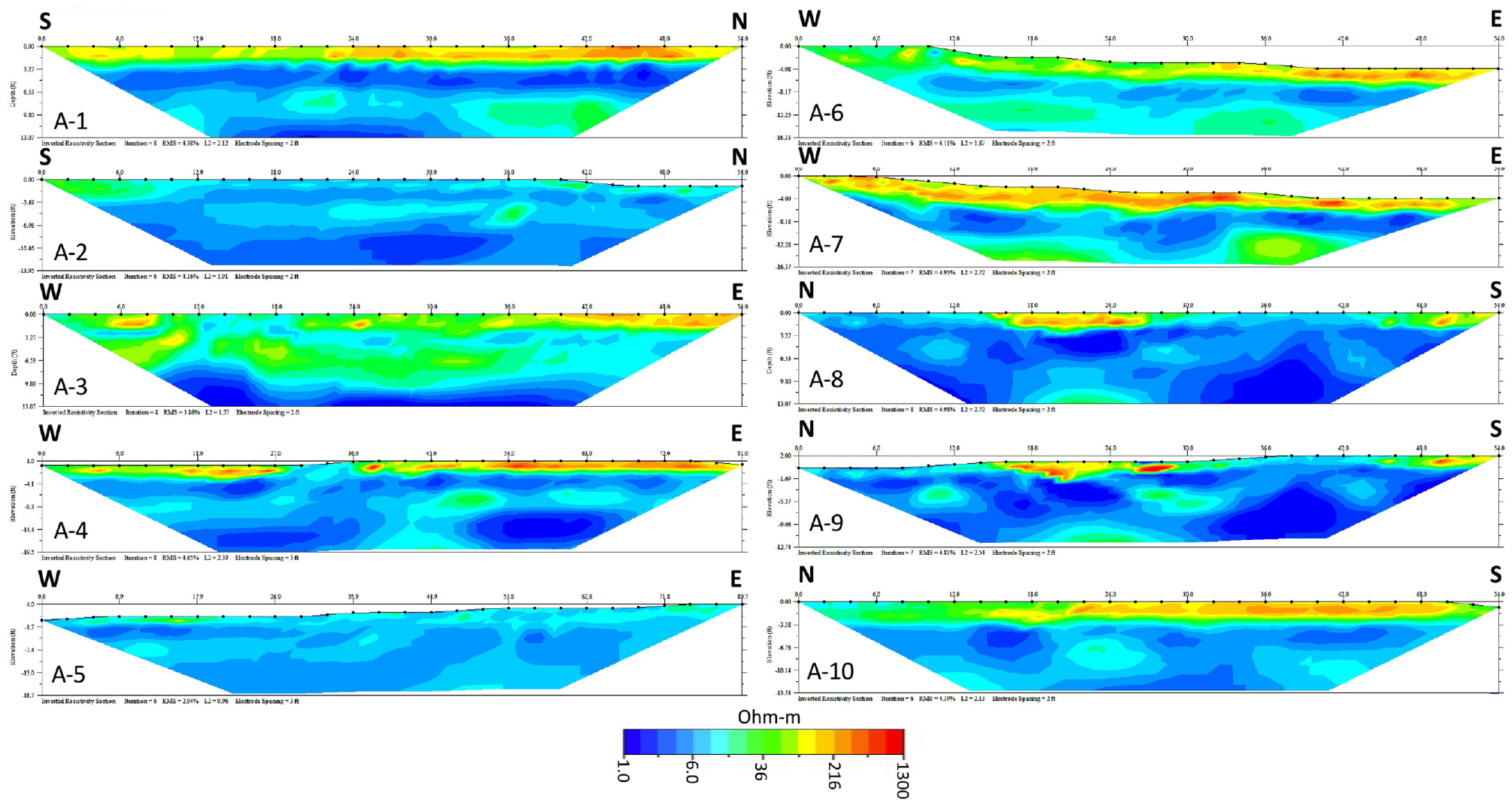
2D inverted resistivity profiles of lines A-1 to A-10.

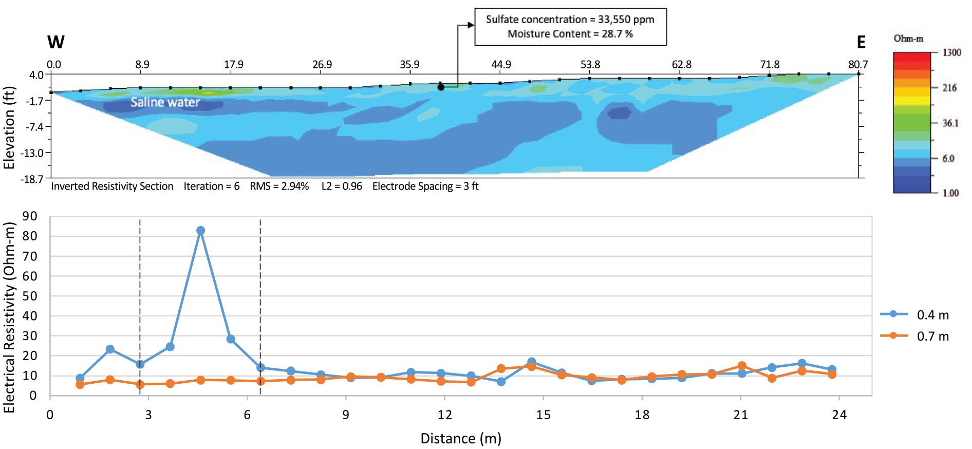
Below is a detailed discussion of five profiles that best represent subsurface conditions at Site 1. Figure 8 illustrates the inverted resistivity profile of line A-2. The electrical resistivity variations along the resistivity profile at a depth from which a soil sample was taken (0.4 m) are also plotted in Figure 8. The borehole BH-1 at a 4.3 m (14 ft) distance shows a layer of crushed limestone at the top, which is underlaid by stiff to very stiff clays up to a depth of 6 m (20 ft). On the other hand, the profile shows low variations in the electrical resistivity between 1 to 50 Ω.m through the length and depth of the profile, indicating the existence of similar earth materials. The inconsistencies between the observations imply that high moisture and sulfate concentration levels exist in the shallow subsurface between 2 and 16 m distance, which is consistent with the borehole results; note that the typical values of electrical resistivity for limestone are larger than 50 Ω.m (Table 1). Soluble sulfate in soils can significantly decrease the resistance of earth materials to a flow of electric currents; however, disaggregation of the impacts of sulfate concentration and moisture content on the variations of electrical resistivity is challenging.

Figure 8.

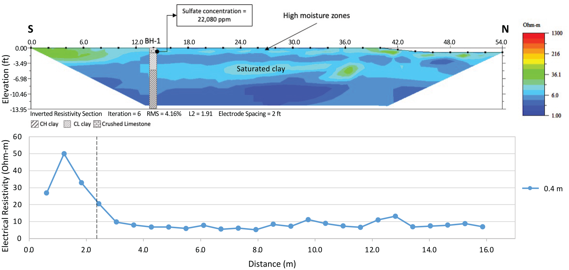
2D resistivity profile of line A-2 and electrical resistivity variations along the profile.

During 15 days before implementing the ERI surveys (April 2022), no precipitation was observed at the study site ( 38 ). The potential groundwater table level is distinguished by vertical changes in the electrical resistivities all along the profile below 1.5 m (5 ft) depth. The high water content in the shallow subsurface is caused by the transition of water from the groundwater table to the soil pores—capillary action ( 39 , 40 ). In silt or clay, the upper boundary of the capillary zone may extend up to a few meters and have an irregular shape ( 39 , 41 ).

Figure 9 shows similar subsurface conditions with line A-2. According to Figure 9, the low resistive areas at the shallow subsurface within a 6 to 24 m (21 to 78 ft) distance are associated with high moisture and sulfate concentration zones that are confirmed by the laboratory test results. The more resistive layer is shown within a distance of 2 to 6 m (6 to 21 ft). The electrical resistivity drops from 83 to 8 Ω.m at 1 m deep. A conductive zone underlies the resistive layer, which indicates a potential area of accumulated sulfate concentrations. The salt minerals are washed through the cracks and accumulate in water zones. The accumulated salts in underlying layers can be transported to the top layer by fluctuations in the groundwater table level and capillarity rise ( 14 ).

Figure 9.

2D resistivity profile of line A-5 and electrical resistivity variations along the profile.

Figure 10 specifies three layers in the subsurface: a resistive layer at the top with electrical resistivities >60 Ω.m (dense crushed limestone), a transition layer with electrical resistivities of about 30 Ω.m, and a conductive layer with electrical resistivities <9 Ω.m. A sharp drop in the electrical resistivities through the depth indicates the potential groundwater table level at approximately 2.5 m (8 ft) below the ground surface. No evidence of high sulfate concentration is observed through the length of the profile up to a depth of about 1 m (3 ft). The results of laboratory tests confirm that the subsurface materials contain low water and sulfate concentrations at a 7 m (24 ft) distance.

Figure 10.

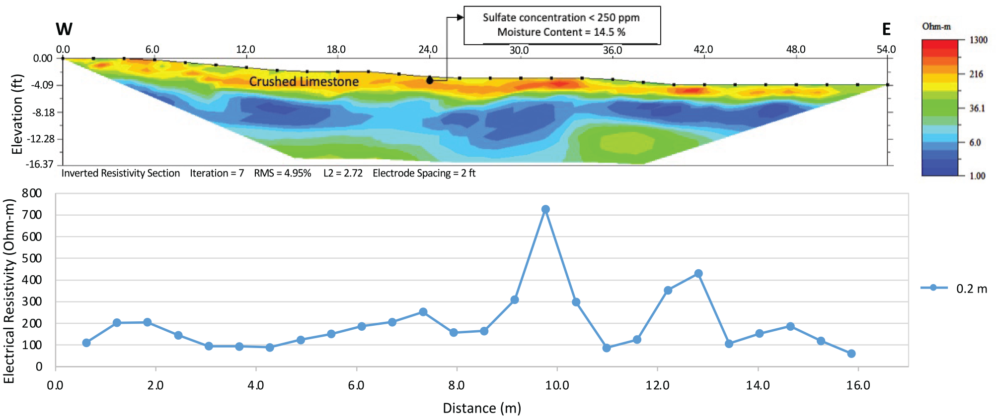
2D resistivity profile of line A-7 and electrical resistivity variations along the profile.

According to Figure 11, two conductive zones with electrical resistivities below 10 Ω.m indicate high levels of moisture and sulfate concentration. The borehole results also show high sulfate concentrations (17,835 ppm) at 0.6 m distance. The more resistive zones centered at 6.5 m and 15 m distance, show no evidence of high sulfate concentrations at the shallow subsurface.

Figure 11.

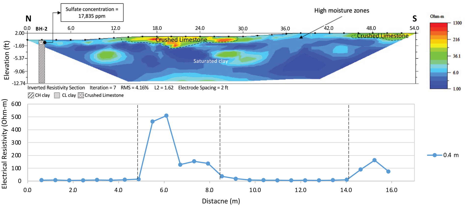
2D resistivity profile of line A-9 and electrical resistivity variations along the profile.

As shown in Figure 12, electrical resistivities at the shallow subsurface vary from 10 Ω.m on the left to 500 Ω.m on the right side of the resistivity profile. According to the laboratory test results (S5 and S6 in Table 2), a less resistive zone at the sampling location is attributed to a moderate sulfate concentration zone. No evidence of high sulfate concentration can be observed between 6.5 to 15 m distance by generalizing the previous findings; however, a conductive zone at the top left corner of the A-10 profile could indicate a high sulfate concentration zone. Potential groundwater table could be found at 4 ft depth.

Figure 12.

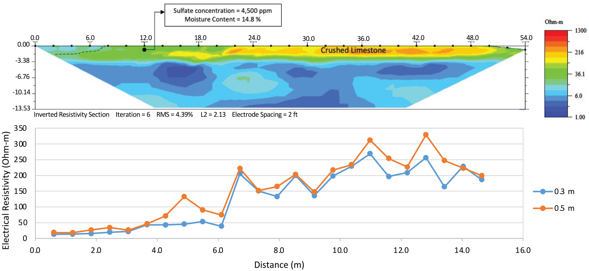
2D resistivity profile of line A-10 and electrical resistivity variations along the profile.

Site 2

Figure 13 shows the 2D inverted resistivity profiles of lines B-1 to B-4. The profiles show consistent subsurface conditions through the depth of profiles, except for line B-4, with electrical resistivity ranging from 1 to 40 Ω.m. Low electrical resistivity variations imply the existence of similar earth materials with similar geotechnical properties. However, according to the site geology, a variety of earth materials (e.g., sand, shale, and clay) can be found at the study site up to 6 m (20 ft) deep. The inconsistency between existing soil layers and ranges of electrical resistivities indicates the high sulfate concentrations all along the profiles. The inverted resistivity profile of line B-4 shows relatively high variations in the electrical resistivities ranging from 1 to 150 Ω.m. The conductive areas (<3 Ω.m) below the resistive top layer indicate saline water zones that increase the risk of sulfate-induced heaving in those locations. The source of water could be an 8 mm (0.33 in.) precipitation at the site two days before conducting the ERI surveys (November 2021) ( 38 ).

Figure 13.

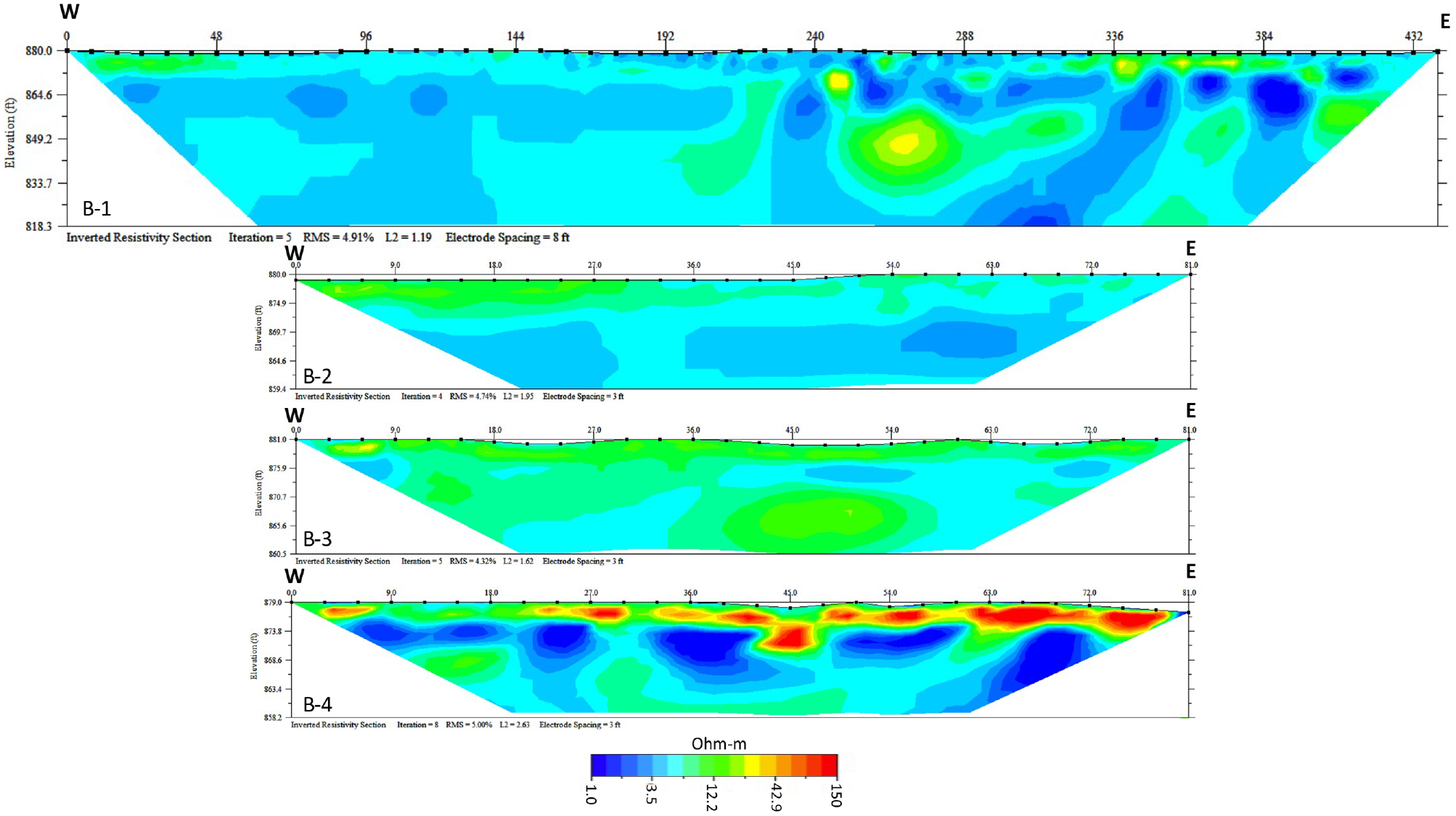
2D inverted resistivity profiles of lines B-1 to B-4.

A discussion of two profiles that best reflect the subsurface conditions at Site 2 is provided below. Figure 14 indicates low variations in the electrical resistivities, ranging from 3 to 18 Ω.m. The borehole data show different earth materials up to about 4.7 m (15.5 ft), consisting of a clayey sand layer (top 0.3 m), soft to hard high plasticity clay with a trace of gypsum lenses (0.3 to 3.7 m), and shale with a trace of calcareous deposits (3.7 to 4.7 m). However, the observed electrical resistivities do not represent clayey sand in the shallow subsurface; the typical range of electrical resistivities for sands is above 10 Ω.m. The low resistive areas at the shallow subsurface show high sulfate concentration areas within a 9 to 24 m (30 to 81 ft) distance, distinguished by a threshold electrical resistivity of 8 Ω.m. The laboratory test results confirm a minimum sulfate concentration of 17,000 ppm at a 12 m (40 ft) distance in the clay layer (S8 in Table 2).

Figure 14.

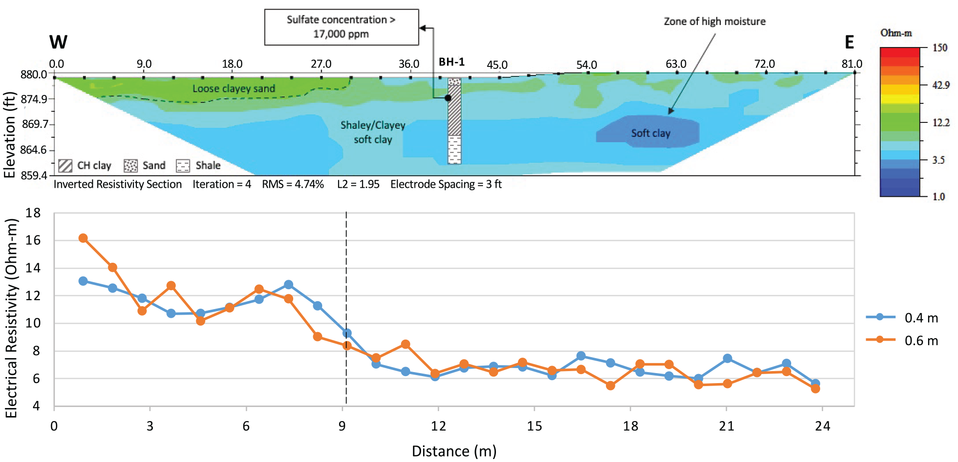
2D resistivity profile of line B-2 and electrical resistivity variations along the profile.

More resistive areas can be observed along line B-3 (Figure 15) than line B-2 (Figure 14) at the shallow subsurface centered at 11 and 23 m (36 and 75 ft) distance. These areas are associated with moist, clayey sands containing low sulfate concentrations. The laboratory test results also agree with the ERI findings (S9 and S10 in Table 2). However, at deeper depths, high sulfate concentration is distinguished by less resistive zones (<5 Ω.m) within clayey soil ( 37 ).

Figure 15.

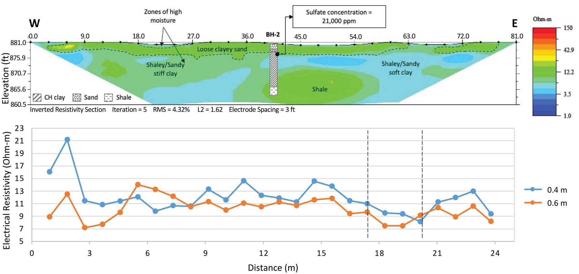
2D resistivity profile of line B-3 and electrical resistivity variations along the profile.

Conclusion

Assessment of the extent and levels of sulfate concentration is still challenging because of the limitations of the current methods in considering the spatial heterogeneity of sulfate minerals in soils and their seasonal fluctuations. ERI has been of interest in assessing the subsurface conditions and providing fill-in information between the measurements. This study aimed to explore the application of ERI in determining the extent and levels of sulfate concentrations. Several ERI surveys were conducted in two sites in Texas with the potential high risk of sulfate-induced heaving. A few soil samples were also collected to determine the sulfate concentrations and moisture contents in the field sites to help validate the ERI results. This study showed that soluble sulfate in soils decreases the electrical resistivities of earth materials below their typical ranges. The results also showed that the reduction in the electrical resistivities for soils with high sulfate concentrations is more significant than for soils with low and moderate sulfate concentrations. The proposed approach could be used by state DOTs to identify areas where traditional methods of site investigation, which are costly and time-consuming, are not necessary.

Although this study identified different limits for differentiating low to high sulfate concentration zones, more investigations need to be performed to generalize the ERI findings for other earth materials. Once the range of electrical resistivities with the sulfate concentration levels is validated at a few locations by the laboratory test results, a continuous assessment of the levels of sulfate concentration could be achieved through a rapid operation for long sections of a highway. It is also intriguing to evaluate the variations of sulfate concentrations at different periods during the wet and dry seasons at the exact locations.

Supplemental Material

sj-pdf-1-trr-10.1177_03611981231167162 – Supplemental material for Electrical Resistivity Imaging for Identifying Critical Sulfate Concentration Zones Along Highways

Supplemental material, sj-pdf-1-trr-10.1177_03611981231167162 for Electrical Resistivity Imaging for Identifying Critical Sulfate Concentration Zones Along Highways by Mina Zamanian, Yatindra Anand Thorat, Natnael Asfaw, Prakash Chavda and Mohsen Shahandashti in Transportation Research Record

Supplemental Material

sj-pdf-2-trr-10.1177_03611981231167162 – Supplemental material for Electrical Resistivity Imaging for Identifying Critical Sulfate Concentration Zones Along Highways

Supplemental material, sj-pdf-2-trr-10.1177_03611981231167162 for Electrical Resistivity Imaging for Identifying Critical Sulfate Concentration Zones Along Highways by Mina Zamanian, Yatindra Anand Thorat, Natnael Asfaw, Prakash Chavda and Mohsen Shahandashti in Transportation Research Record

Supplemental Material

sj-pdf-3-trr-10.1177_03611981231167162 – Supplemental material for Electrical Resistivity Imaging for Identifying Critical Sulfate Concentration Zones Along Highways

Supplemental material, sj-pdf-3-trr-10.1177_03611981231167162 for Electrical Resistivity Imaging for Identifying Critical Sulfate Concentration Zones Along Highways by Mina Zamanian, Yatindra Anand Thorat, Natnael Asfaw, Prakash Chavda and Mohsen Shahandashti in Transportation Research Record

Supplemental Material

sj-pdf-4-trr-10.1177_03611981231167162 – Supplemental material for Electrical Resistivity Imaging for Identifying Critical Sulfate Concentration Zones Along Highways

Supplemental material, sj-pdf-4-trr-10.1177_03611981231167162 for Electrical Resistivity Imaging for Identifying Critical Sulfate Concentration Zones Along Highways by Mina Zamanian, Yatindra Anand Thorat, Natnael Asfaw, Prakash Chavda and Mohsen Shahandashti in Transportation Research Record

Footnotes

Acknowledgements

The authors are grateful to TxDOT for supporting this work and for their valuable feedback.

Author Contributions

The authors confirm their contribution to the paper as follows: study conception and design: MZ, NA, PC, MS; data collection: MZ, YTA; analysis and interpretation of results: MZ, MS; draft manuscript preparation: MZ, MS, NA, PC. All authors reviewed the results and approved the final version of the manuscript.

Declaration of Conflicting Interests

The author(s) declared no potential conflicts of interest with respect to the research, authorship, and/or publication of this article.

Funding

The author(s) disclosed receipt of the following financial support for the research, authorship, and/or publication of this article: This study was supported by the Texas Department of Transportation (Project No. 5-7008-01).

ORCID iDs

Mina Zamanian

Natnael Asfaw

Mohsen Shahandashti

Data Accessibility Statement

The data that support the findings of this study are available from the corresponding author on reasonable request.

Supplemental Material

Supplemental material for this article is available online.

References

Puppala

A. J.

Intharasombat

Vempati

R. K.

Experimental Studies on Ettringite-Induced Heaving in Soils. Journal of Geotechnical and Geoenvironmental Engineering, Vol. 131, No. 3, 2005, pp. 325–337.

Puppala

A. J.

Wattanasanticharoen

Intharasombat

Hoyos

L. R.

Studies to Understand Soil Compositional and Environmental Variables on Sulfate Heave Problems. Proc., Soil Rock America, 12th Pan American Conference on Soil Mechanics and Geotechnical Engineering, Cambridge, MA, 2003.

Puppala

An Innovative Hybrid Sensor for Rapid Assessment of Sulfate-Induced Heaving in Stabilized Soils. NCHRP-IDEA Program Project Final Report. Transportation Research Board, Washington, D.C., 2013.

Chen

D. H.

Harris

Scullion

Bilyeu

Forensic Investigation of a Sulfate-Heaved Project in Texas. Journal of Performance of Constructed Facilities, Vol. 19, No. 4, 2005, pp. 324–330.

Adams

A. G.

Dukes

O. M.

Tabet

Cerato

A. B.

Miller

G. A.

Sulfate Induced Heave in Oklahoma Soils Due to Lime Stabilization. Proc., GeoCongress 2008: Characterization, Monitoring, and Modeling of GeoSystems, American Society of Civil Engineers, Reston, VA, 2008, pp. 444–451.

Talluri

Stabilization of High Sulfate Soils. Civil & Environmental Engineering, Arlington, TX, 2013.

Shahandashti

Mattingly

Darghiasi

Baral

Abediniangerabi

Snowplow Operations Management System. No. FHWA/TX-22/5-6996-01-1. Texas Department of Transportation, Research and Technology Implementation Office, Austin, 2022.

Baral

Shahandashti

Risk-Averse Rehabilitation Decision Framework for Roadside Slopes Vulnerable to Rainfall-Induced Geohazards. Journal of Infrastructure Preservation and Resilience, Vol. 3, No. 1, 2022, pp. 1–13.

Baral

Shahandashti

S. M.

Identifying Critical Combination of Roadside Slopes Susceptible to Rainfall-Induced Failures. Natural Hazards, Vol. 113, No. 2, 2022, pp. 1177–1198.

10.

Darghiasi

Baral

Abediniangerabi

Shahandashti

A Multi-Purpose All-in-One Mobile Data Collection System for Snowplow Operation Management. Proc., International Conference on Transportation and Development, Seattle, WA, 2022, American Society of Civil Engineers, pp. 39–50.

11.

Darghiasi

Baral

Mattingly

Shahandashti

Estimation of Road Surface Temperature Using NOAA Gridded Forecast Weather Data for Snowplow Operations Management. Journal of Cold Regions Engineering. Forthcoming 2023. https://doi.org/10.1061/JCRGEI/CRENG-691.

12.

Darghiasi

Baral

Shahandashti

Developing a Cost-Effective Mobile-Based System for Collecting On-Demand Road Condition Images for Snowplow Operations Management. Proc., International Conference on Transportation and Development, Austin, TX, Forthcoming 2023.

13.

Guidelines for Treatment of Sulfate-Rich Soils and Bases in Pavement Structures. Texas Department of Transportation (TxDOT), 2005. www.ftp.dot.state.tx.us/pub/txdot-info/cmd/tech/sulfates.pdf. Accessed July 14, 2022.

14.

National Academies of Sciences, Engineering, and Medicine. Recommended Practice for Stabilization of Sulfate-Rich Subgrade Soils. The National Academies Press, Washington, D.C., 2009. https://doi.org/10.17226/22997.

15.

Harris

Harvey

Sebesta

Rapid Field Detection of Sulfate and Organic Content in Soils. Technical Report No. FHWA/TX-11/0-6362-1. Texas Transportation Institute, College Station, 2011.

16.

Shon

C. S.

Sebesta

Scullion

Implementation of Technology for Rapid Field Detection of Sulfate and Organic Content in Soils. Technical Report No. FHWA/TX-12/5-6362-01-1. Texas Transportation Institute, College Station, 2012.

17.

Muñoz

Felicísimo

Á. M.

Comparison of Statistical Methods Commonly Used in Predictive Modelling. Journal of Vegetation Science, Vol. 15, No. 2, 2004, pp. 285–292.

18.

Shahandashti

Hossain

Zamanian

Akhtar

M. A.

Advanced Geophysical Tools for Geotechnical Analysis. No. FHWA/TX-20/0-7008-1. Texas Department of Transportation, Austin, 2021.

19.

Zamanian

Asfaw

Chavda

Shahandashti

Classifying Soil Sulfate Concentration Using Electrical Resistivity Imaging and Random Forest Algorithm. Proc., International Airfield Highway Pavements Conference, Austin, TX, Forthcoming 2023.

20.

Moral

F. J.

Terrón

J. M.

DaSilva

J. M.

Delineation of Management Zones Using Mobile Measurements of Soil Apparent Electrical Conductivity and Multivariate Geostatistical Techniques. Soil and Tillage Research, Vol. 106, No. 2, 2010, pp. 335–343.

21.

Austin District Pavement Design Standard Operating Procedures. Texas Department of Transportation (TxDOT), 2021. https://ftp.txdot.gov/pub/txdot/aus/specinfo/district-pavement-design-sop.pdf. Accessed July 14, 2022.

22.

Bheemasetti

T. V.

Chittoori

Zou

Puppala

A. J.

Thomey

Spatial Mapping of Soluble Sulfate Concentrations Present in Natural Soils Using Geostatistics. Journal of Geotechnical and Geoenvironmental Engineering, Vol. 143, No. 2, 2017, p. 04016090.

23.

Akingboye

A. S.

Ogunyele

A. C.

Insight into Seismic Refraction and Electrical Resistivity Tomography Techniques in Subsurface Investigations. Rudarsko-geološko-naftni zbornik (The Mining-Geological-Petroleum Engineering Bulletin), Vol. 34, No. 1, 2019. https://doi.org/10.17794/rgn.2019.1.9.

24.

Bernard

Leite

Vermeersch

Instruments

I. R.

Orleans

Multi-Electrode Resistivity Imaging for Environmental and Mining Applications. IRIS Instruments, Orléans, France, 2006.

25.

Loke

M. H.

Tutorial: 2-D and 3-D Electrical Imaging Surveys. 2004. https://sites.ualberta.ca/∼unsworth/UA-classes/223/loke_course_notes.pdf.

26.

Hossain

Kibria

Khan

Site Investigation Using Resistivity Imaging. CRC Press, London, 2018.

27.

Gomaa

M. M.

Salinity and Water Effect on Electrical Properties of Fragile Clayey Sandstone. Applied Water Science, Vol. 10, No. 5, 2020, pp. 1–9.

28.

Zamanian

Shahandashti

Investigation of Relationship Between Geotechnical Parameters and Electrical Resistivity of Sandy Soils. Proc., Construction Research Congress, Arlington, VA, 2022, American Society of Civil Engineers, pp. 686–695.

29.

Advanced Geosciences, Inc. Instruction Manual for EarthImager 2D, Version 2.4.0. Resistivity and IP Inversion Software, Austin, TX, 2009.

30.

Milsom

Field Geophysics, Vol. 31. John Wiley & Sons, New York, NY, 2003.

31.

The Society of Exploration Geophysicists of Japan. Application of Geophysical Methods to Engineering and Environmental Problems. The Society of Exploration Geophysicists of Japan, Tokyo, 2004.

32.

Day-Lewis

F. D.

Johnson

C. D.

Singha

Lane

J. W.

Best Practices in Electrical Resistivity Imaging: Data Collection and Processing, and Application to Data from Corinna, Maine. EPA Report. CLU-IN.org, Boston, MA, 2008.

33.

Zarroca

Bach

Linares

Pellicer

X. M.

Electrical Methods (VES and ERT) for Identifying, Mapping and Monitoring Different Saline Domains in a Coastal Plain Region (Alt Empordà, Northern Spain). Journal of Hydrology, Vol. 409, No. 1–2, 2011, pp. 407–422.

34.

Margiotta

Negri

Parise

Quarta

T. A. M.

Karst Geosites at Risk of Collapse: The Sinkholes at Nociglia (Apulia, SE Italy). Environmental Earth Sciences, Vol. 75, No. 1, 2016, pp. 1–10.

35.

Arjwech

Electrical Resistivity Imaging for Unknown Bridge Foundation Depth Determination. Doctoral dissertation. Texas A&M University, College Station, 2011.

36.

Loke

M. H.

RES2DINVx64 ver. 4.05: Rapid 2-D Resistivity & IP Inversion Using the Least-Squares Method. Geotomosoft Solutions, Geotomo Software PTY LTD, 2015.

37.

Goebel

Pidlisecky

Knight

Resistivity Imaging Reveals Complex Pattern of Saltwater Intrusion Along Monterey Coast. Journal of Hydrology, Vol. 551, 2017, pp. 746–755.

38.

Weather Underground. 2022. www.wunderground.com. Accessed July 14, 2022.

39.

Shen

Pennell

K. G.

Suuberg

E. M.

Influence of Soil Moisture on Soil Gas Vapor Concentration for Vapor Intrusion. Environmental Engineering Science, Vol. 30, No. 10, 2013, pp. 628–637.

40.

Zhang

Gao

Y. X.

Feng

Zhang

Y. Z.

Liu

J. C.

Zhang

Y. P.

Experimental Study on Height Simulation of Capillary Fringe. Journal of Groundwater Science and Engineering, Vol. 8, No. 2, 2020, pp. 108–117.

41.

Hodson

W. G.

Geology and Ground-Water Resources of Mitchell County, Kansas. Printed in the State Printing Plant, University of Kansas, 1959.

Supplementary Material

Please find the following supplemental material available below.

For Open Access articles published under a Creative Commons License, all supplemental material carries the same license as the article it is associated with.

For non-Open Access articles published, all supplemental material carries a non-exclusive license, and permission requests for re-use of supplemental material or any part of supplemental material shall be sent directly to the copyright owner as specified in the copyright notice associated with the article.

0.00 MB

0.09 MB

0.11 MB