Sage Journals: Discover world-class research

Abstract

Electrical resistivity imaging is gaining popularity in aiding the characterization of subsurface conditions and assessment of the stability of earth materials. Nevertheless, it remains challenging to identify the relationship between geotechnical properties and electrical resistivities because of their nonlinear and complex relationship. This study intends to assess the application of the deep learning model to explore the relationship between electrical resistivities and geotechnical properties of natural clayey soils. A full factorial design was used to study the effects of water content and dry unit weight on the electrical resistivities of soils composed of different fractions of fine and clay particles. A deep learning model with three hidden layers was trained using a dataset comprising 842 observations to investigate the association between electrical resistivities and geotechnical properties. Influencing geotechnical properties were identified by Spearman’s correlation and feature importance. The results show that most variabilities in the electrical resistivity can be explained by the water content and dry unit weight. The results also show that the plasticity index and fine fraction play a more substantial role in predicting the electrical resistivities of clayey soils than the liquid limit and clay fraction. A comparison between the accuracy metrics of the deep learning model with existing models in the literature shows that deep learning outperforms other models in discovering nonlinear and complex relationships between electrical resistivities and geotechnical properties. Enhanced knowledge of the relationship between geotechnical properties and electrical resistivities allows for better characterizing the subsurface conditions to improve reliability and reduce uncertainties caused by inadequate subsurface information.

Keywords

artificial intelligence deep learning infrastructure soil and rock properties subsurface exploration transportation systems resilience

Successful design and construction of infrastructure projects highly depend on the adequate characterization of subsurface conditions ( 1 , 2 ). Continuous mapping of earth materials in project sites on which infrastructure will be erected is crucial for the optimized design, construction, and maintenance of infrastructures, including highways and bridges ( 3 , 4 ). Conventional geotechnical site investigation methods provide accurate information about the subsurface conditions; however, this information is limited to specific locations in the field sites (i.e., point-specific data) ( 5 , 6 ). Because of heterogeneity and anisotropy, generalizing borehole information to the entire space between the boreholes may lead to incorrect interpretations, structural failures, interruptions in the project schedule, and additional labor or material costs ( 7 – 10 ). Since state transportation agencies have limited budgets for road maintenance activities ( 11 ), advanced geophysical techniques, such as electrical resistivity imaging, are used alongside conventional geotechnical site investigation methods to provide additional information between the boreholes to mitigate the maintenance costs.

Electrical resistivity imaging measures the soil resistance to an electrical current—soil electrical resistivity. Soil electrical resistivity is a function of the soil and rock matrix, degree of saturation, pore fluid conductivity, soil fabric structure, and soil compressibility ( 12 – 14 ). Among the hydraulic properties, soil water content plays a significant role in the variability of electrical resistivity since electrical current can easily be transmitted through the movement of ions in pore water ( 15 , 16 ). Shahandashti et al. ( 1 ) showed that 66% of the total variations of the electrical resistivity are attributed to variations in water content. Also, the degree of saturation and void ratio (one of the controlling factors of water content) significantly affect electrical resistivity variations ( 17 , 18 ). The variability of electrical resistivity is less sensitive to the variations of dry unit weight than the water content. An increase in dry density results in less pore space and more interparticle contacts, decreasing soil resistance to electrical current flow. Rashid et al. ( 19 ) observed a 50% reduction in electrical resistivity for a 20% increase in the dry density. However, the reduction rate in electrical resistivity with increasing dry density depends on the soil type. Besides, in soils characterized by a high plasticity index and liquid limit, a low electrical resistivity value is anticipated ( 17 , 20 ); the plasticity index shows a more significant correlation with the electrical resistivity of clayey soils than the liquid limit. Soils with a higher percentage of fines (percent of soil finer than 75 µm) and clays (percent of soil finer than 2 µm) yield lower electrical resistivity values because they have higher specific surface areas, which promotes the transmission of electrical current ( 21 ). Because of the correlation between electrical resistivity and geotechnical properties, electrical resistivity imaging offers a continuous assessment of subsurface conditions and identifies weak zones prone to failure ( 1 , 22 , 23 ). For instance, electrical resistivity can be used to estimate water content ( 24 ), determine the degree of compaction ( 25 ), detect and locate slope failures ( 26 ), estimate the soil liquefaction potential ( 27 ), and identify groundwater and soil pollution ( 28 ). Nevertheless, it remains challenging to determine the relationship between electrical resistivities and geotechnical properties because of the simultaneous effects of multiple geotechnical properties on electrical resistivities, which have complex relationships with one another ( 22 , 29 ).

Artificial intelligence (AI) techniques have the potential to revolutionize the designs, construction, and maintenance of infrastructure systems by providing advanced analytics, automation, and predictive capabilities ( 30 – 32 ). Researchers have employed AI techniques, such as linear regressions, artificial neural networks (ANNs), and support vector machines (SVMs), to establish relationships between geotechnical properties and electrical resistivities. Linear regressions have been widely used to quantify electrical resistivity variabilities based on geotechnical properties ( 33 ). The purpose of linear regression is to construct mathematical models that explain the relationships between two or more variables ( 34 ). Shahandashti et al. ( 1 ) adopted multivariate linear regressions (MLRs) to investigate the relationships among electrical resistivity with water content, dry unit weight, plasticity index, and fine fraction in clayey soils. By performing regression analysis and examining diagnostic tests, they found that the electrical resistivities have a nonlinear relationship with the geotechnical properties ( 1 ). Although linear regressions are easy to implement and their results are simple to interpret, they are incapable of handling the nonlinear relationship between input and output variables present in the electrical resistivity data. Alsharari et al. ( 35 ) compared the performance of MLRs with nonlinear regressions and ANNs in quantifying the electrical resistivity based on water content, dry unit weight, pore water salinity, and percentage of fine and coarse grains of soil samples synthetically made. They found that nonlinear regressions perform better than linear regressions in explaining the nonlinear and complex interdependencies between the electrical resistivities and geotechnical properties; however, both models show higher prediction errors than ANNs. Other researchers also explored the applicability of ANNs in predicting soil electrical resistivity based on geotechnical properties. Bian et al. ( 22 ) adopted ANNs to estimate electrical resistivities based on water content, degree of saturation, and porosity. In a similar study, Rashid et al. ( 19 ) performed an experimental study to investigate the variations in the electrical resistivities of kaolinite-dominant clay liners caused by variations in water content and dry unit weight. They developed ANNs to predict electrical resistivities and concluded that ANNs could be used to assess the level of heterogeneity of compacted clay liners. Samui ( 36 ) examined the application of SVMs and least square support vector machines (LSSVMs) in investigating the associations among electrical resistivity and soil thermal resistivity, the coarse-grained fraction, and the degree of saturation. He compared the accuracy of the developed SVMs and LSSVMs with ANNs and found that the SVMs and LSSVMs outperform the ANNs, with a slightly better performance of LSSVMs over SVMs. Likewise, Samui ( 37 ) found that ANNs do not perform as well as Gaussian process regression (GPR) in quantifying the soil electrical resistivities based on the soil thermal resistivity, degree of saturation, and coarse-grained fraction. Although ANNs are more flexible at handling nonlinear interactions between the variables, feature extraction and feature engineering are still necessary before training the networks to improve prediction accuracy. In other words, ANNs cannot derive meaningful features from unprocessed data because of their shallow structures ( 38 ).

Identifying the relationship between geotechnical properties and electrical resistivities is a complex problem ( 22 , 29 ). The current methods for determining electrical resistivity based on geotechnical properties pose two challenges: (1) the application of linear models such as MLR cannot reveal the nonlinear relationship between the input and output variables, and (2) the application of nonlinear models with shallow structures such as ANNs does not allow them to efficiently represent highly nonlinear patterns in the electrical resistivity data ( 39 ). Therefore, this paper explores the application of a deep learning model that can consider a high level of nonlinearity and complexity of interactions between electrical resistivities and geotechnical properties, such as the water content, plasticity index, dry unit weight, and fine fraction in clayey soils. The deep learning model performance is then evaluated and compared with the performance of ANNs, SVMs, and linear regressions. This research’s findings help better identify the influence of geotechnical properties on electrical resistivities. Enhanced knowledge of the relationship between geotechnical properties and electrical resistivities allows for better characterizing the subsurface conditions to improve reliability and reduce uncertainties caused by inadequate subsurface information.

Research Approach

This research assesses the application of deep learning modeling in investigating the relationship between geotechnical properties and electrical resistivities. The research approach comprises four main parts: (1) design of experiments; (2) performing laboratory electrical resistivity and soil physical property tests to collect data; (3) developing a deep learning model for estimating electrical resistivities based on geotechnical properties of clayey soils, such as the water content, plasticity index, dry unit weight, and fine fraction; and (4) comparing the trained deep learning model performance with the performance of ANNs, SVMs, and linear regressions. Figure 1 illustrates a flow diagram for the approach followed in this research.

Figure 1.

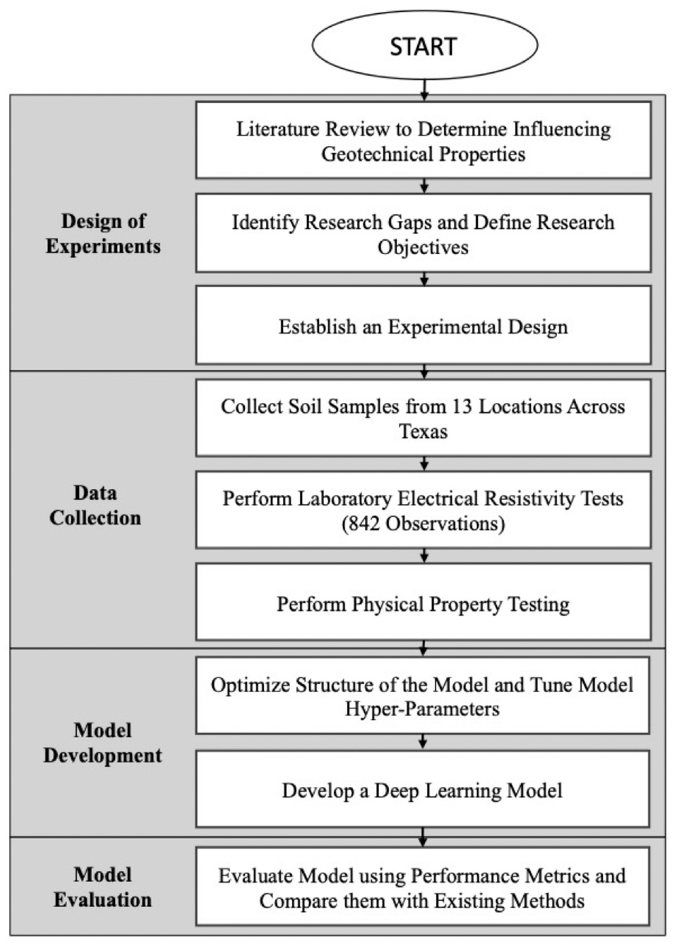
Research approach flow diagram.

Design of Experiments

A full factorial design was established to investigate the effects of water content and dry unit weight on the electrical resistivity of various soil samples with different fractions of fine and clay particles. A full factorial design generates observations by all possible combinations of factor levels in each complete experiment; it is particularly useful in studying the factor effects when the number of factors is less than five ( 40 , 41 ). The water content and dry unit weight were studied at four and three levels. The factors and corresponding factor levels are shown in Table 1. The design resulted in at least 12 experimental runs for each soil sample.

Table 1.

Factors and Corresponding Factor Levels in the Experimental Design

Factor	Unit	Factor levels
Factor	Unit	1	2	3	4
Water content	%	10	20	30	40
Dry unit weight	$kN / m^{3}$	11.8	13.4	14.9	na

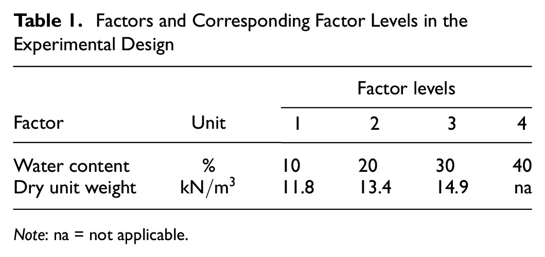
Note: na = not applicable.

Laboratory Testing

A total of 57 soil samples were obtained using wet rotary methods from 13 sites in five different districts across Texas to study the effects of the influencing geotechnical properties on the electrical resistivities of clayey soil. Figure 2 shows the locations of soil sample collection on the Texas map. These sites are located within a distance of up to 680 km.

Figure 2.

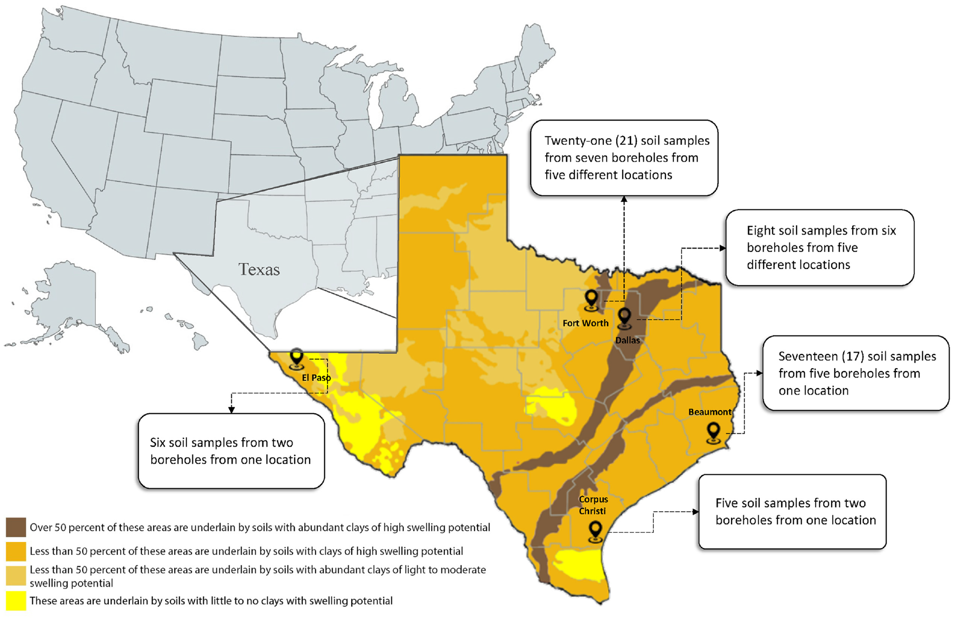
Locations of the soil sample collection on the Texas map.

Based on the experimental design, each soil sample was mixed with different amounts of water in the laboratory. Soil samples were then compacted in a soil box with three compaction efforts to conduct the electrical resistivity tests. A total of 842 observations were obtained using an AGI SuperSting R8 instrument following the standard test method for measuring electrical resistivity ( 42 ). The measured electrical resistivity of soil is dependent on the cross-sectional area of the soil box and electrode spacings ( 42 ) and can be expressed by $ρ = \frac{A R}{d}$ , where $ρ$ is electrical resistivity (Ω.m), A is the cross-sectional area of the soil box perpendicular to the current flow (m²), d is the inner distance between the potential electrodes (m), and R is the electrical resistance according to Ohm’s law.

In addition to the laboratory electrical resistivity measurements, soil physical property tests were conducted to quantify the plasticity index, fine fraction (particles smaller than sieve no. 200), clay fraction (particles smaller than 2 µm), and specific gravity of the soil samples. Table 2 summarizes the basic statistics (e.g., range of values, mean, variance) of the measured parameters. According to Table 2, the soil samples are classified as low (CL) to high (CH) plasticity clayey soils based on the unified soil classification system (USCS).

Table 2.

Basic Statistics of the Input and Output Variables

Parameters	Abbreviation	Minimum value	Maximum value	Mean	VAR	n
Water content	$ω$ (%)	6.6	66.0	24.1	125.7	842
Dry unit weight	$γ_{d} (kN / m^{3})$	7.8	15.8	12.7	1.3	842
Plasticity index	$PI$ (%)	6.5	46.5	28.4	65.6	842
Fine fraction	$F$ (%)	54.2	98.0	85.7	94.5	842
Clay fraction	C (%)	9.4	68.8	43.3	188.2	842
Specific gravity	$G_{s}$	2.6	2.72	2.65	0.001	842
Electrical resistivity	$ρ (Ω . m)$	2.3	995.0	27.3	5394.1	842

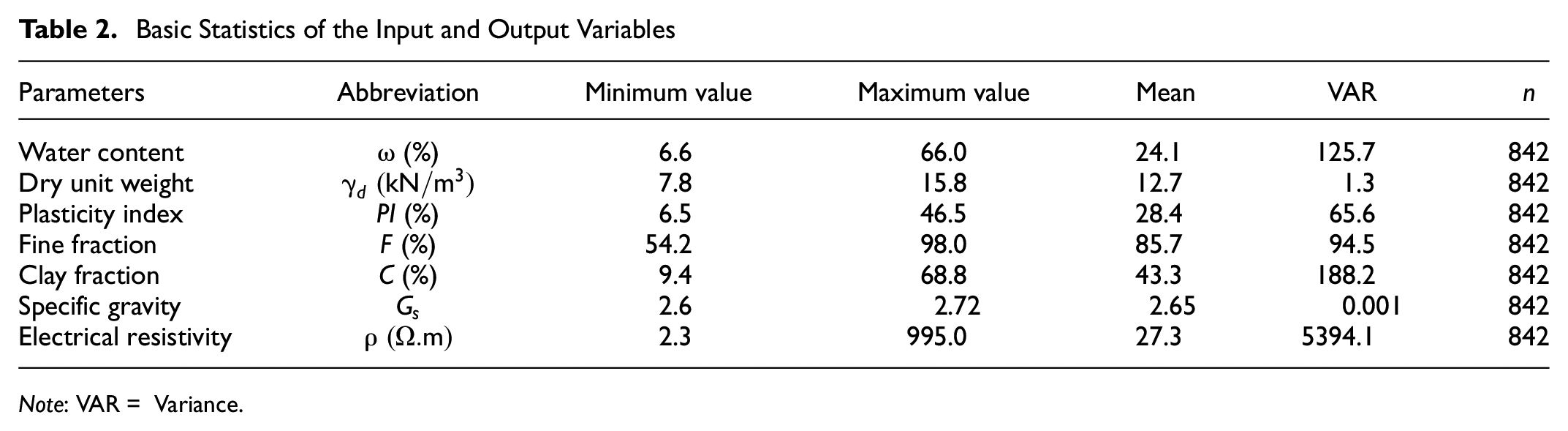
Note: VAR = Variance.

Deep Learning Model

ANNs mimic the biological learning mechanism of the human brain, enabling the exploration of intricate and nonlinear associations between input and output variables ( 38 ). The neural networks consist of a single input layer, one or multiple hidden layers, and a single output layer. Each layer comprises one or more neurons, and each layer’s neurons are interconnected to neurons at the subsequent layer by weighted connections. The neurons process elements of a neural network and resemble human brain cells ( 43 ). The networks that contain more than one hidden layer are called “deep learning” or “deep neural networks” (DNNs). Figure 3 shows the structure of the deep learning models developed for this study. The deep learning models use simple but nonlinear algorithms to extract multiple higher levels of representation from the raw data and reveal complex patterns ( 44 ). While shallow and DNNs possess the universal approximation property, research shows that deep network architectures, which consist of two or more hidden layers, outperform shallow network architectures, which consist of only one hidden layer, with an exponentially lower number of training parameters ( 45 ).

Figure 3.

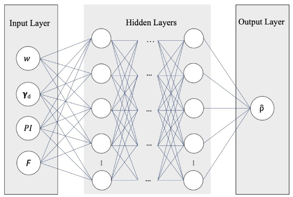
Structure of deep learning models.

The neural networks represent and compute the nonlinear associations between the input and output features in the hidden layers ( 23 ). Each hidden layer’s neuron uses a nonlinear activation function to establish a relationship between the input and output variables. Mathematically, a combination of the nonlinear weighted sum is approximated by Equation 1:

f (X) = ϕ (W^{T} X + b)

(1)

where X is the matrix of input variables, $ϕ$ is the activation function, W is the vector of neuron weights, and b is the bias term at a hidden layer. The commonly utilized activation functions in the neurons of hidden layers include the rectifier linear unit (ReLU), hyperbolic tangent, and sigmoid functions. Computationally, the ReLU function exhibits a faster learning rate than sigmoid and hyperbolic tangent functions in DNNs ( 46 ), since it does not saturate the output to a given value by increasing or decreasing the input variables ( 47 ). This study employed the ReLU function in all neurons of the hidden layers except for the last hidden layer. Instead, a linear function was used to connect the last hidden layer to the output layer. A backpropagation learning algorithm is extensively exploited for training the networks, involving a feedforward and a backward process ( 23 ). In the feedforward process, the past observations are fed into the input layer and then propagated to the hidden layers to extract further information. The connection weights are determined to transfer the extracted information to the output layer to predict the outputs. The backward process updates the connection weights and biases based on the predicted outputs and actual values. The training cycle of the networks is repeated many times to find the optimal combination of weights that will yield the optimal output for any input variable ( 48 ).

As discussed earlier, geotechnical properties, such as the degree of saturation and porosity, exhibit strong pairwise correlations with electrical resistivity values ( 49 ). Nevertheless, when exploring the simultaneous associations of geotechnical parameters with electrical resistivity, these properties insignificantly improve the performance accuracy of the model because of their interrelations with water content and dry unit weight. Moreover, incorporating numerous inputs into the model may result in excessive complexity and, consequently, lead to overfitting ( 50 ). In this study, deep learning models were trained by four input geotechnical properties, namely the water content, plasticity index, dry unit weight, and fine fraction, to estimate the soil electrical resistivities. The data were standardized by subtracting the mean from all observations and then scaling to unit variance to speed up the model training, which is essential when dealing with a large volume of data ( 51 ). The data were randomly split into two sets by a ratio of 80 to 20 before model training. In other words, 80% of the observations were used to train the deep learning models, and the remaining 20% of the observations were used to evaluate the model accuracies. Three hidden layers were chosen for deep learning models to ensure the best accuracy of the model ( 52 ). The maximum number of hidden layer neurons is determined by 2I+ 1, where I represents the number of input variables ( 53 ). Therefore, the optimum number of neurons for the hidden layers was selected based on trial-and-error by altering the number of neurons from one to nine. The selection of many hidden layers and neurons within layers could result in overfitting (i.e., high variance) if the level of complexity of the problem is disregarded ( 54 ). The model with the minimum root mean square of error (RMSE) and mean absolute error (MAE) for the testing dataset was then selected as the optimal model. The hyperparameters of the model, such as the epoch number and batch size, were chosen based on a grid search using 10-fold cross-validation with a learning rate of 0.001. In the n-fold cross-validation method, the training data is divided into n equal parts (i.e., folds). The model is trained based on n−1 parts and then evaluated on the remaining part. The process is repeated n times until every part is used once for validation ( 55 ). The performance of the final model is then calculated by averaging the results of each iteration ( 56 ). Table 3 presents the ranges of the model hyperparameters used in the grid search. The batch size was also examined in conjunction with the execution time of the training process ( 38 ).

Table 3.

Model Hyperparameter Ranges in the Grid Search

Hyperparameters	Values
Number of neurons in different layers	8, 8, 9
Number of epochs	10, 20, 30, 40, 50, 100, 150, 200, 300, 400, 500
Batch sizes	64, 128
Activation function	ReLU, linear
Optimizer	Adam
Learning rate	0.001
Losses	RMSE, MAE

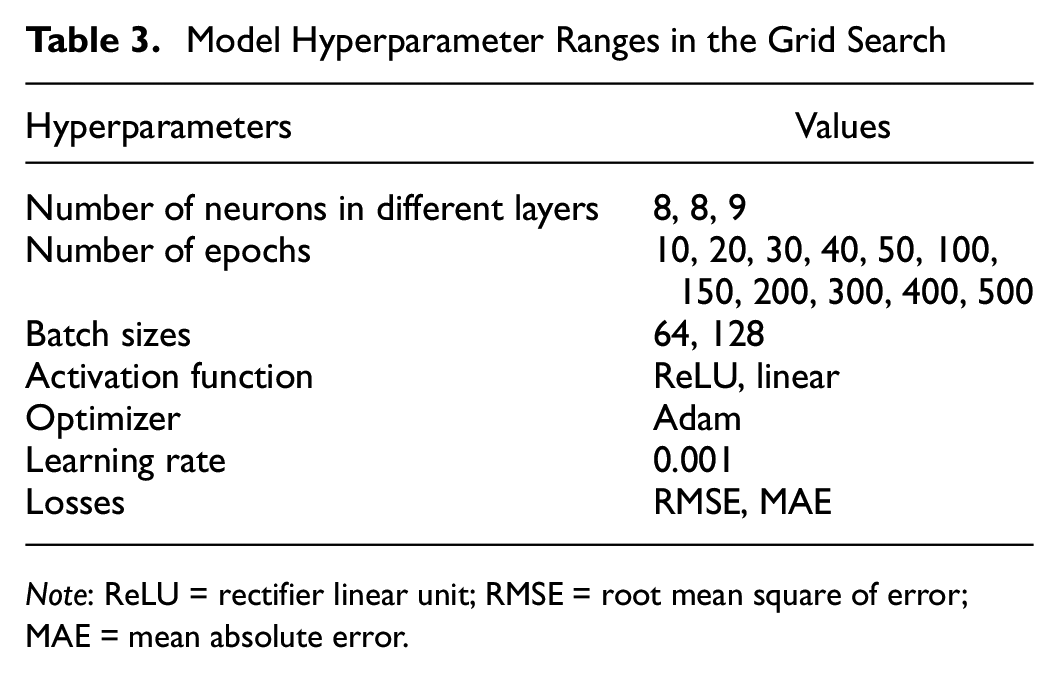
Note: ReLU = rectifier linear unit; RMSE = root mean square of error; MAE = mean absolute error.

As a result, a deep learning model composed of three hidden layers with eight (first hidden layer), eight (second hidden layer), and nine (third hidden layer) neurons was adopted to evaluate the applicability of DNNs in determining the associations between the geotechnical properties and electrical resistivities in clayey soils.

Research Results and Discussion

Descriptive Statistics

This section provides descriptive analyses of the data obtained by laboratory experiments to identify the most influencing factors affecting electrical resistivities. Figure 4 illustrates the frequency histograms of the measured geotechnical properties of the soil samples. According to Figure 4, all geotechnical properties show a wide range of values (i.e., high variance), except for the specific gravity. The high variance in the geotechnical properties (i.e., water content, plasticity index, dry unit weight, fine fraction, and clay fraction) indicates that these variables can be useful in determining the variance of the electrical resistivity.

Figure 4.

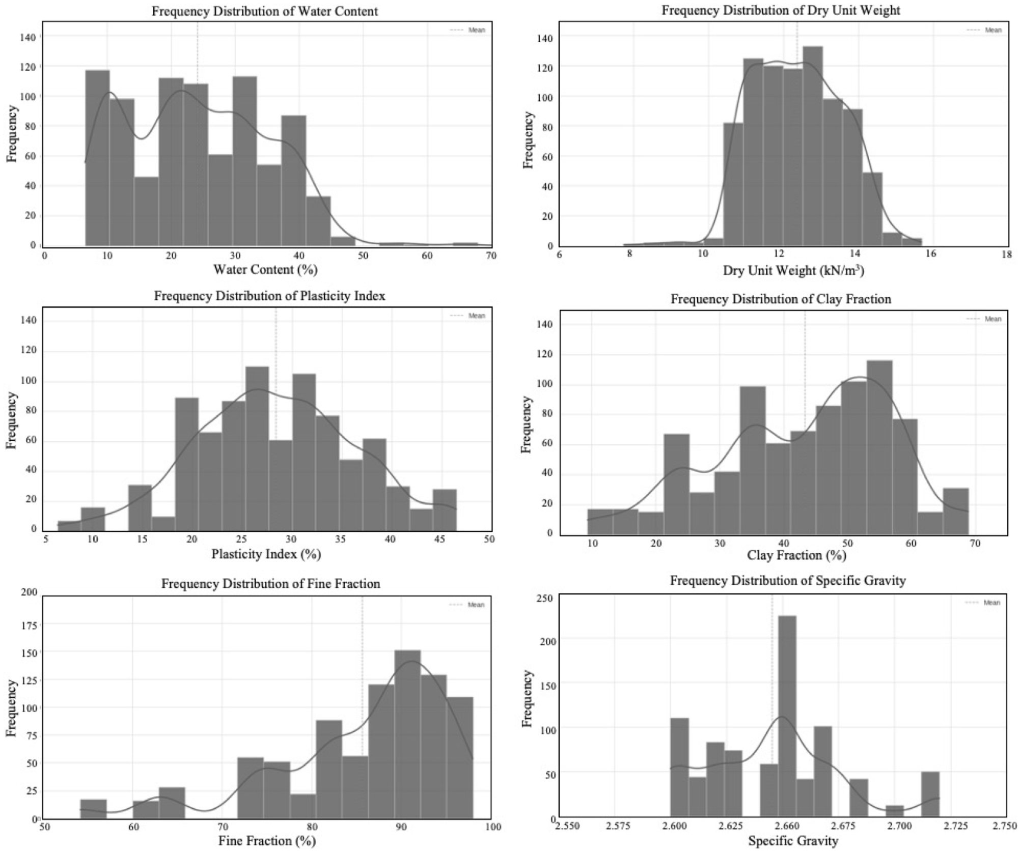
Frequency distribution of the geotechnical properties of soil samples.

Moreover, Spearman’s correlation analysis was performed to assess the strength of the pairwise relationships between electrical resistivities and geotechnical properties. Spearman’s correlation evaluates the existence of a monotonic dependence between the ranked values of two variables, without assuming linearity of the relationship ( 57 ). Figure 5 presents Spearman’s correlation coefficients for the electrical resistivity and geotechnical properties on a heatmap. Spearman’s coefficients range between −1 and 1. A positive coefficient indicates monotonic changes in the same direction, whereas a negative coefficient shows monotonic changes in the opposite direction ( 58 ). According to Figure 5, electrical resistivity indicates a strong inverse correlation with the water content (r_s = −0.77). In other words, the electrical resistivity of soil significantly decreases with an increase in the water content. The literature also confirms that the water content inversely influences the electrical resistivity of clayey or sandy soils ( 15 , 35 ). Based on Figure 5, electrical resistivity shows weak correlations with the dry unit weight, plasticity index, fine fraction, and clay fraction. Note that Spearman’s correlation solely measures the degree of a monotonic relationship between two variables. However, there might be strong non-monotonic relationships between the variables that cannot be captured by Spearman’s correlation ( 59 ).

Figure 5.

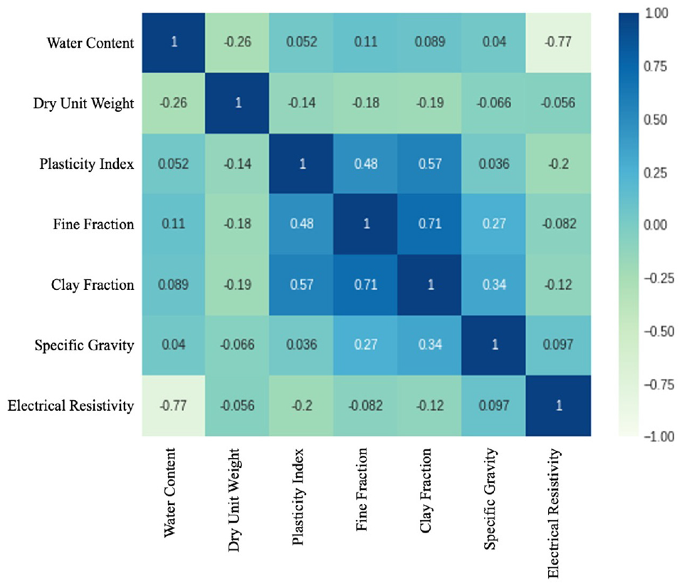
Spearman’s correlation coefficient heatmap of the electrical resistivity and geotechnical properties.

Deep Learning Results

A deep learning model consisting of three hidden layers was constructed, with the layers containing eight, eight, and nine neurons, respectively. Four geotechnical properties, namely water content, plasticity index, dry unit weight, and fine fraction, were fed into the neurons of the input layer to estimate the soil electrical resistivities. Figure 6 illustrates the training and testing loss functions (mean squared and absolute errors) for the developed deep learning model across different epochs, ranging from 1 up to 500. The epoch upper limit was set to the highest possible value to ensure that the loss functions converge during the training process ( 38 ). According to Figure 6, the deep learning loss functions converge to a constant value as the number of epochs increases. The mean squared error (MSE) and MAE loss functions start to saturate around the same value and converge in about 100 epochs. The fluctuations observed on the training and testing curves do not affect the model’s overall accuracy ( 60 ).

Figure 6.

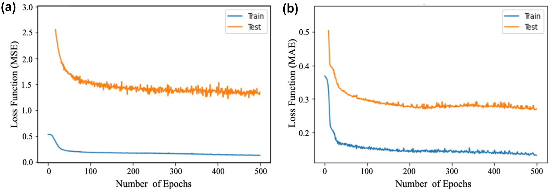
Training and testing loss functions of developed deep learning model: (a) mean squared error (MSE) and (b) mean absolute error (MAE).

Validating black-box models such as deep learning requires an understanding of the underlying relationships between input and output variables, which can be achieved by extracting features’ importance ( 61 ). Figure 7 illustrates the relative importance of each geotechnical property in predicting the electrical resistivities. A geotechnical property that contributes to more substantial losses in the model is assigned a higher importance score. Conversely, a feature with a score close to zero indicates the minimal impact of that feature on the predictions. According to Figure 7, water content exhibits the highest level of influence on the variability in the electrical resistivities. This finding also aligns with the results of Spearman’s correlation analysis. The results are consistent with the literature, which identifies water content as the primary factor affecting electrical resistivities ( 30 , 62 ). Pore water facilitates the passage of an electrical current through pore spaces by moving ions, which reduces Earth’s resistance ( 24 ). Shahandashti et al. ( 1 ) showed that about 66% of the variability of electrical resistivity can be explained by the water content. Moreover, Figure 7 indicates that the dry unit weight is the second most influencing geotechnical property affecting the electrical resistivity variations, following water content. Although this finding contradicts the result of the correlation analysis, which shows a weak correlation between the dry unit weight and electrical resistivity, the existing literature shows that the dry unit weight is useful in explaining the variability in the electrical resistivities ( 1 , 35 ). Changes in dry unit weights result in changes in pore spaces and interparticle contacts. Therefore, especially at low water contents, continuous pathways for the flow of electrical current can be created at high dry unit weights, which result in lower electrical resistivities ( 19 ). The plasticity index and fine fraction demonstrate significant but the least important scores among the other geotechnical properties, implying that they have lower impacts on the electrical resistivity predictions. Lin et al. ( 25 ) also found some correlations between the electrical resistivity of clayey soils and the plasticity index. Theoretically, fine-grained soil yields lower electrical resistivities than coarse-grained soil because they have higher specific surface areas, which promotes the transmission of an electrical current ( 21 ).

Figure 7.

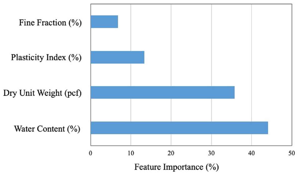
Relative importance of geotechnical properties in predicting electrical resistivity.

Model Comparison of Deep Learning Model with the ANN, the SVM, and MLR

A deep learning model with an optimal number of hidden layers (i.e., three layers) and hidden layer neurons (i.e., 8, 8, and 9 neurons) was adopted in this study to assess the applicability of DNNs in investigating the nonlinear and complex relationships between electrical resistivities and geotechnical properties. Four geotechnical properties, namely the water content, plasticity index, dry unit weight, and fine fraction, were fed into the neurons of the input layer to estimate the soil electrical resistivities.

The performance of the trained deep learning model was evaluated and compared to an ANN, a SVM, and MLR. An ANN was trained through 100 iterations to compare the performance of the shallow with deep network architectures in investigating the associations between electrical resistivities and geotechnical properties. The ANN comprises a single input layer with four neurons (i.e., water content, plasticity index, dry unit weight, and fine fraction), a single hidden layer with nine neurons, and a single output layer with one neuron (i.e., electrical resistivity). The number of neurons in hidden layers was chosen based on trial-and-error by changing the number of neurons from one to nine and examining the model accuracy for the testing dataset. A SVM with a radial basis function kernel was also trained to predict electrical resistivities using the same geotechnical properties. The radial basis function kernel transforms the nonlinear relationship between the input and output variables into a linear relationship within a higher-dimensional space. The adopted deep learning model, ANN, and SVM were compared to the multiple linear regression developed by Shahandashti et al. ( 1 ). A Box–Cox and a natural log transformation were used on the input and output variables to satisfy the linear regression assumptions (i.e., linearity, homoskedasticity, and normality) ( 1 ).

Figure 8 illustrates the measured and predicted electrical resistivities for the training and testing datasets by deep learning, ANN, SVM, and multiple linear regression models. The accuracy of the deep learning model (R-squared) is about 87% for the training and 70% for the testing datasets. According to Figure 8, it is concluded that the deep learning model shows more prediction accuracy on both the training and testing datasets when compared to other models. Moreover, the results imply that the deep learning model with three hidden layers is more robust than the other methods. In other words, because of the slight difference between the training and testing accuracies for deep learning, it is concluded that the model performance remains approximately the same for predicting out-of-sample data. On the other hand, the MLR shows the worst performance for the training and testing datasets.

Figure 8.

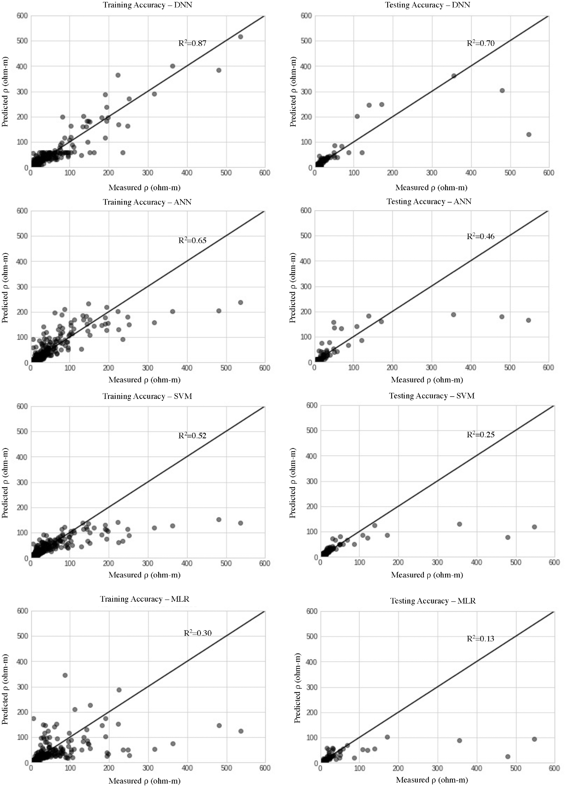
Training and testing accuracies for the developed deep learning, artificial neural network (ANN), support vector machine (SVM), and multivariate linear regression (MLR) models to predict the electrical resistivities.

Figure 9 shows the testing accuracy of deep learning, ANN, SVM, and MLR models for predicting electrical resistivity based on RMSE and MAE metrics. The testing accuracies show the outperformance of the deep learning model compared with the other models in predicting the electrical resistivities, with a RMSE of 68.9 and MAE of 17.8, followed by the ANN with a RMSE of 92.9 and MAE of 23.4. The outperformance of the deep learning model compared with the ANN is because of the ability of deep network architectures to discover more complex patterns and interactions between the input and output variables compared with shallow network architectures. Compared with all other methods, linear regression shows the most significant errors, with a RMSE of 115.5 and MAE of 25.7. The low performance of the multiple linear regression is because of its inability to handle the nonlinear and complex relationship between electrical resistivities and geotechnical properties.

Figure 9.

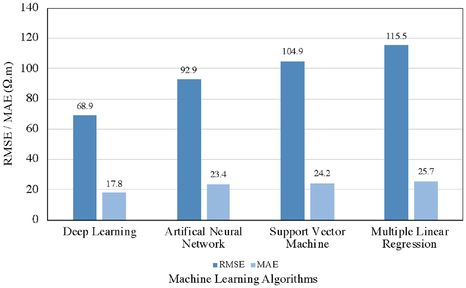
Accuracy metrics of the deep neural network, artificial neural network, support vector machine, and multiple linear regression for the testing dataset.

Conclusion

Accurate characterization of geotechnical properties and their variabilities in space is still challenging because of the heterogeneity of earth materials and the limitations of conventional geotechnical site investigation methods. Electrical resistivity imaging complements the geotechnical site investigation methods by providing fill-in data between the boreholes. However, there is a lack of an analytical tool for exploring the complex and nonlinear relationship between electrical resistivities and geotechnical properties. This research is the most rigorous study conducted on natural clayey soils to examine the applicability of the deep learning model to discover complex and nonlinear relationships between electrical resistivities and geotechnical properties. A full factorial experiment was performed to investigate the effects of different levels of water content and dry unit weight on the variabilities of electrical resistivity. A total of 842 laboratory electrical resistivity tests were conducted on 57 disturbed soil samples obtained from different locations across Texas.

This study developed a deep learning model comprising three hidden layers (with 8, 8, and 9 neurons in the hidden layers, respectively) to investigate the associations between electrical resistivities and geotechnical properties. The pairwise dependence of variables was analyzed by Spearman’s correlation. Besides, the relative importance of the geotechnical properties in predicting the electrical resistivities was derived from the trained model. The performance of the deep learning model was then compared to the performance of the ANN, SVM, and multiple linear regression. The results showed that the water content makes a significant contribution to the predictions of the electrical resistivities in clayey soils. The findings of this study show that the dry unit weight plays a crucial role in electrical resistivity variations, which can be attributed to the pore spaces that provide pathways for the electrical current. Furthermore, the results illustrated that the electrical resistivity of clayey soils is more influenced by the percentage of fines and plasticity index than the clay fraction and liquid limit. This study found that the deep learning model provides more accurate estimates for electrical resistivity compared to all other methods, with a RMSE of 68.9 and MAE of 17.8. This study also showed that the deep learning model yields a more robust and generalized model since there is a slight difference between the training and testing accuracies. The outperformance of the deep learning model compared with the ANN indicates a high level of complexity among the geotechnical properties and electrical resistivities. This research’s findings help one to better understand the variability of electrical resistivities caused by changes in geotechnical properties. The proposed methodology offers a means to enhance subsurface characterization for assessing the engineering properties of clayey soil, such as undrained shear strength ( 63 ), based on the electrical resistivities with a rapid and cost-effective method. In addition, this methodology can be applied to ascertain the salinity of pore water ( 25 ) and potentially identify zones with critical sulfate concentration ( 5 , 30 ). Such information is crucial for implementing effective subgrade stabilization methods. The proposed methodology helps in calibrating electrical resistivity images by utilizing geotechnical properties at specific points. This approach enhances the reliability of subsurface condition interpretations. Moreover, the research results can be applied to other applications where a comprehensive understanding of electrical resistivity and its relationship with the geotechnical properties is essential, such as the design of grounding systems ( 64 ).

While this research provided a practical recommendation for implementing a deep learning model in investigating the relationship between geotechnical properties and electrical resistivities and revealed a high level of complexity among the electrical resistivity data, this research is subjected to multiple limitations. The practical recommendations for developing deep learning models in this research are limited to multivariate prediction models based on experimental data. Nevertheless, continuous geotechnical data are not always available from the field sites. In future work, it is of interest to integrate the proposed approach with a technique that leverages publicly available data to determine unknown geotechnical properties that show minimal variations over time, such as the fine fraction, to simplify the developed machine learning models. Consequently, to be practically implemented, pairwise relationships between electrical resistivity and geotechnical properties may be established. Secondly, to further improve the model inference, it is recommended that calibration of unknown parameters is performed if output data is available ( 65 ). In addition, it is encouraged to report the uncertainties associated with calibrated parameters and use them in probability-based analyses ( 66 ). Therefore, it is of interest to calibrate the adopted deep learning model using the observed data from boreholes to minimize the errors of the model and provide the most accurate outputs that are consistent with the observed data.

Footnotes

Author Contributions

The authors confirm contribution to the paper as follows: study conception and design: M. Zamanian, N. Asfaw, P. Chavda, M. Shahandashti; data collection: M. Zamanian, N. Asfaw, P. Chavda, M. Shahandashti; analysis and interpretation of results: M. Zamanian, M. Shahandashti; draft manuscript preparation: M. Zamanian, M. Shahandashti, N. Asfaw, P. Chavda. All authors reviewed the results and approved the final version of the manuscript.

Declaration of Conflicting Interests

The author(s) declared no potential conflicts of interest with respect to the research, authorship, and/or publication of this article.

Funding

The author(s) disclosed receipt of the following financial support for the research, authorship, and/or publication of this article: This study is based on work supported by the Texas Department of Transportation (TxDOT) (Projects No. 0-7008-01). The authors are grateful to TxDOT for supporting this work.

ORCID iDs

Mina Zamanian

Natnael Asfaw

Mohsen Shahandashti

Data Accessibility Statement

The data that support the findings of this study are available from the corresponding author on reasonable request.

References

Shahandashti

Hossain

Zamanian

Akhtar

M. A.

Advanced Geophysical Tools for Geotechnical Analysis. No. FHWA/TX-20/0-7008-1. Texas Department of Transportation, Research and Technology Implementation Office, Austin, 2021.

Cosenza

Marmet

Rejiba

Cui

Y. J.

Tabbagh

Charlery

Correlations Between Geotechnical and Electrical Data: A Case Study at Garchy in France. Journal of Applied Geophysics, Vol. 60, No. 3-4, 2006, pp. 165–178.

Baral

Shahandashti

S. M.

A Data Integration Approach for Assessment of Rainfall-Induced Slope Failure Susceptibility. Proc., Construction Research Congress, Arlington, VA, American Society of Civil Engineers, 2022, pp. 480–489.

Shahandashti

Mattingly

Darghiasi

Baral

Abediniangerabi

Snowplow Operations Management System. No. FHWA/TX-22/5-6996-01-1. Texas Department of Transportation, Research and Technology Implementation Office, Austin, 2022.

Zamanian

Thorat

Y. A.

Asfaw

Chavda

Shahandashti

Electrical Resistivity Imaging for Identifying Critical Sulfate Concentration Zones Along Highways. Transportation Research Record: Journal of the Transportation Research Board, 2023. 2677: 113–127.

Shahandashti

Hossain

Zamanian

Implementation of Electrical Resistivity Imaging Manual. No. FHWA/TX-24/5-7008-01-1. Texas Department of Transportation. Research and Technology Implementation Office, Austin, 2023.

Darghiasi

Baral

Abediniangerabi

Shahandashti

A Multi-Purpose All-in-One Mobile Data Collection System for Snowplow Operation Management. Proc., International Conference on Transportation and Development, Seattle, WA, American Society of Civil Engineers, 2022, pp. 39–50.

Shahandashti

Hossain

Baral

Adhikari

Pourmand

Abediniangerabi

Slope Repair and Maintenance Management System. No. FHWA/TX-20/5-6957-01-1. Texas Department of Transportation, Research and Technology Implementation Office, Austin, 2022.

Baral

Sadegh Nasr

Darghiasi

Abediniangerabi

Shahandashti

Detection and Classification of Vegetation for Roadside Vegetation Inspection and Rehabilitation Using Deep Learning Techniques. Proc., International Conference on Transportation and Development, Seattle, WA, American Society of Civil Engineers, 2022, pp. 143–152.

10.

Adiat

K. A. N.

Relevance of Electrical Resistivity Geophysical Method in Engineering Site Characterization in a Basement Complex Terrain. Global Journal of Engineering Sciences, Vol. 2, No. 1, 2019, pp. 1–6.

11.

Darghiasi

Baral

Shahandashti

Developing a Cost-Effective Mobile-Based System for Collecting On-Demand Road Condition Images for Snowplow Operations Management. Proc., International Conference on Transportation and Development, Austin, TX, American Society of Civil Engineers, 2023, pp. 127–137.

12.

Ekwue

E. I.

Bartholomew

Electrical Conductivity of Some Soils in Trinidad as Affected by Density, Water and Peat Content. Biosystems Engineering, Vol. 108, No. 2, 2011, pp. 95–103.

13.

Friedman

S. P.

Soil Properties Influencing Apparent Electrical Conductivity: A Review. Computers and Electronics in Agriculture, Vol. 46, No. 1-3, 2005, pp. 45–70.

14.

Samouëlian

Cousin

Tabbagh

Bruand

Richard

Electrical Resistivity Survey in Soil Science: A Review. Soil and Tillage Research, Vol. 83, No. 2, 2005, pp. 173–193.

15.

Zamanian

Shahandashti

Investigation of Relationship between Geotechnical Parameters and Electrical Resistivity of Sandy Soils. Proc., Construction Research Congress, Arlington, VA, American Society of Civil Engineers, 2022, pp. 686–695.

16.

Besson

Cousin

Bourennane

Nicoullaud

Pasquier

Richard

Dorigny

King

The Spatial and Temporal Organization of Soil Water at the Field Scale as Described by Electrical Resistivity Measurements. European Journal of Soil Science, Vol. 61, No. 1, 2010, pp. 120–132.

17.

Abu-Hassanein

Z. S.

Benson

C. H.

Blotz

L. R.

Electrical Resistivity of Compacted Clays. Journal of Geotechnical Engineering, Vol. 122, No. 5, 1996, pp. 397–406.

18.

Rinaldi

V. A.

Cuestas

G. A.

Ohmic Conductivity of a Compacted Silty Clay. Journal of Geotechnical and Geoenvironmental Engineering, Vol. 128, No. 10, 2002, pp. 824–835.

19.

Rashid

Q. A.

Abuel-Naga

H. M.

Leong

E. C.

Al Abadi

Experimental-Artificial Intelligence Approach for Characterizing Electrical Resistivity of Partially Saturated Clay Liners. Applied Clay Science, Vol. 156, 2018, pp. 1–10.

20.

Long

Donohue

L’Heureux

J. S.

Solberg

I. L.

Rønning

J. S.

Limacher

O’Connor

Sauvin

Rømoen

Lecomte

Relationship Between Electrical Resistivity and Basic Geotechnical Parameters for Marine Clays. Canadian Geotechnical Journal, Vol. 49, No. 10, 2012, pp. 1158–1168.

21.

Morin

R. H.

Negative Correlation Between Porosity and Hydraulic Conductivity in Sand-and-Gravel Aquifers at Cape Cod, Massachusetts, USA. Journal of Hydrology, Vol. 316, No. 1-4, 2006, pp. 43–52.

22.

Bian

Liu

Cai

Tian

Artificial Neural Network Model for Predicting Soil Electrical Resistivity. Journal of Intelligent & Fuzzy Systems, Vol. 29, No. 5, 2015, pp. 1751–1759.

23.

Erzin

Rao

B. H.

Patel

Gumaste

S. D.

Singh

D. N.

Artificial Neural Network Models for Predicting Electrical Resistivity of Soils from Their Thermal Resistivity. International Journal of Thermal Sciences, Vol. 49, No. 1, 2010, pp. 118–130.

24.

Siddiqui

F. I.

Osman

S. B. A. B. S.

Simple and Multiple Regression Models for Relationship Between Electrical Resistivity and Various Soil Properties for Soil Characterization. Environmental Earth Sciences, Vol. 70, No. 1, 2013, pp. 259–267.

25.

Lin

Cai

Liu

Puppala

A. J.

Zou

Correlations Between Electrical Resistivity and Geotechnical Parameters for Jiangsu Marine Clay Using Spearman’s Coefficient Test. International Journal of Civil Engineering, Vol. 15, No. 3, 2017, pp. 419–429.

26.

Friedel

Thielen

Springman

S. M.

Investigation of a Slope Endangered by Rainfall-Induced Landslides Using 3D Resistivity Tomography and Geotechnical Testing. Journal of Applied Geophysics, Vol. 60, No. 2, 2006, pp. 100–114.

27.

Banimahd

Yasrobi

S. S.

Woodward

P. K.

Artificial Neural Network for Stress–Strain Behavior of Sandy Soils: Knowledge Based Verification. Computers and Geotechnics, Vol. 32, No. 5, 2005, pp. 377–386.

28.

Kim

Y. S.

M. H.

Park

Analysis of Resistivity Data Obtained from Cone Penetrometer in Contaminated Soil Layers. Environmental Geology, Vol. 58, No. 6, 2009, pp. 1309–1317.

29.

Zhang

Liu

Chen

Ding

Application of Deep Learning Algorithms in Geotechnical Engineering: A Short Critical Review. Artificial Intelligence Review, Vol. 54, No. 9, 2021, pp. 1–41.

30.

Zamanian

Asfaw

Chavda

Shahandashti

Classifying Soil Sulfate Concentration Using Electrical Resistivity Imaging and Random Forest Algorithm. Proc., Airfield and Highway Pavements, Austin, TX, American Society of Civil Engineers, 2023, pp. 204–213.

31.

Darghiasi

Baral

Abediniangerabi

Makhmalbaf

Shahandashti

Multilevel Optimization of UHP-FRC Sandwich Panels for Building Façade Systems. In Handbook of Artificial Intelligence in Performance-Driven Design (N. Abbasabadi and M. Ashayeri, eds.), Wiley, 2023.

32.

Baral, A., P. Darghiasi, and M. Shahandashti. Risk-Averse Maintenance Decision Framework for Roadside Slopes Along Highway Corridors. Proc., International Conference on Transportation and Development, Austin, TX, American Society of Civil Engineers, 2023, pp. 383–392.

33.

Zamanian

Darghiasi

Shahandashti

Empirical Study of the Correlation Between Geoelectrical and Soil-Index Properties of Clayey Soils. Proc., Construction Research Congress, Des Moines, IA, American Society of Civil Engineers, 2024.

34.

Seber

G. A.

Lee

A. J.

Linear Regression Analysis, Vol. 329. John Wiley & Sons, Hoboken, NJ, 2012.

35.

Alsharari

Olenko

Abuel-Naga

Modeling of Electrical Resistivity of Soil Based on Geotechnical Properties. Expert Systems with Applications, Vol. 141, 2020, p. 112966.

36.

Samui

Applicability of Data Mining Techniques for Predicting Electrical Resistivity of Soils Based on Thermal Resistivity. International Journal of Geomechanics, Vol. 13, No. 5, 2013, pp. 692–697.

37.

Samui

Utilization of Gaussian Process Regression for Determination of Soil Electrical Resistivity. Geotechnical and Geological Engineering, Vol. 32, 2014, pp. 191–195.

38.

Abediniangerabi

Makhmalbaf

Shahandashti

Deep Learning for Estimating Energy Savings of Early-Stage Facade Design Decisions. Energy and AI, Vol. 5, 2021, p. 100077.

39.

Peng

Albuquerque

P. H. M.

Kimura

Saavedra

C. A. P. B.

Feature Selection and Deep Neural Networks for Stock Price Direction Forecasting Using Technical Analysis Indicators. Machine Learning with Applications, Vol. 5, 2021, p. 100060.

40.

Antony

Design of Experiments for Engineers and Scientists. Elsevier, London, 2014, pp. 63–85.

41.

Davim

J. P.

(Ed.). Mechatronics and Manufacturing Engineering: Research and Development. Elsevier, Amsterdam, 2012.

42.

ASTM G57-20. Standard Test Method for Measurement of Soil Resistivity Using the Wenner Four-Electrode Method. ASTM International, West Conshohocken, PA, 2020.

43.

Darghiasi

Zamanian

Shahandashti

Enhancing Winter Maintenance Decision Making Through Deep Learning-Based Road Surface Temperature Estimation. Proc., Construction Research Congress 2024, Des Moines, IA, 2024.

44.

LeCun

Bengio

Hinton

Deep Learning. Nature, Vol. 521, 2015, pp. 436–444.

45.

Bengio

LeCun

Scaling Learning Algorithms Towards AI. Large-Scale Kernel Machines, Vol. 34, No. 5, 2007, pp. 1–41.

46.

Ang

B. W.

Multiplicative Structural Decomposition Analysis of Aggregate Embodied Energy and Emission Intensities. Energy Economics, Vol. 65, 2017, pp. 137–147.

47.

Achieng

K. O.

Modelling of Soil Moisture Retention Curve Using Machine Learning Techniques: Artificial and Deep Neural Networks vs Support Vector Regression Models. Computers & Geosciences, Vol. 133, 2019, p. 104320.

48.

Caglar

Arman

The Applicability of Neural Networks in the Determination of Soil Profiles. Bulletin of Engineering Geology and the Environment, Vol. 66, No. 3, 2007, pp. 295–301.

49.

Zamanian

Exploring Spatial Associations and Complex Interactions Between Geotechnical Properties and Electrical Resistivity Values in Clayey Soils. Doctoral dissertation. The University of Texas at Arlington, 2023.

50.

Peng

Nagata

M. H.

An Empirical Overview of Nonlinearity and Overfitting in Machine Learning Using COVID-19 Data. Chaos, Solitons & Fractals, Vol. 139, 2020, p. 110055.

51.

Jayalakshmi

Santhakumaran

Statistical Normalization and Back Propagation for Classification. International Journal of Computer Theory and Engineering, Vol. 3, No. 1, 2011, pp. 1793–8201.

52.

Choldun

Santoso

Surendro

Determining the Number of Hidden Layers in Neural Network by Using Principal Component Analysis. Proc., SAI Intelligent Systems Conference, London, Springer, 2019, pp. 490–500.

53.

Caudill

Neural Networks Primer, Part III. AI Expert, Vol. 3, No. 6, 1988, pp. 53–59.

54.

Uzair

Jamil

Effects of Hidden Layers on the Efficiency of Neural Networks. In Proc., IEEE 23rd International Multitopic Conference (INMIC), Pakistan, IEEE, New York, NY, 2020, pp. 1–6.

55.

Darghiasi

Baral

Mattingly

Shahandashti

Estimation of Road Surface Temperature Using NOAA Gridded Forecast Weather Data for Snowplow Operations Management. Journal of Cold Regions Engineering, Vol. 37, No. 4, 2023, p. 04023018.

56.

Hastie

Tibshirani

Friedman

J. H.

The Elements of Statistical Learning: Data Mining, Inference, and Prediction, Vol. 2, Springer, New York, 2009, pp. 1–758.

57.

Deebani

Kachouie

N. N.

Monte Carlo Ensemble Correlation Coefficient for Association Detection. Communications in Statistics-Simulation and Computation, Vol. 51, No. 12, 2022, pp. 7095–7109.

58.

Schober

Boer

Schwarte

L. A.

Correlation Coefficients: Appropriate Use and Interpretation. Anesthesia & Analgesia, Vol. 126, No. 5, 2018, pp. 1763–1768.

59.

Griessenberger

Trutschnig

Junker

R. R.

qad: An R-package to Detect Asymmetric and Directed Dependence in Bivariate Samples. Methods in Ecology and Evolution, Vol. 13, No. 10, 2022. pp. 2138–2149.

60.

Zhang

Xie

Zhang

Qiu

The Adoption of Deep Neural Network (DNN) to the Prediction of Soil Liquefaction Based on Shear Wave Velocity. Bulletin of Engineering Geology and the Environment, Vol. 80, No. 6, 2021, pp. 5053–5060.

61.

Zhong

Zhang

Bagheri

Burken

J. G.

, et al. Machine Learning: New Ideas and Tools in Environmental Science and Engineering. Environmental Science & Technology, Vol. 55, No. 19, 2021, pp. 12741–12754.

62.

Robinson

D. A.

Campbell

C. S.

Hopmans

J. W.

Hornbuckle

B. K.

Jones

S. B.

Knight

Ogden

Selker

Wendroth

Soil Moisture Measurement for Ecological and Hydrological Watershed-Scale Observatories: A Review. Vadose Zone Journal, Vol. 7, No. 1, 2008, pp. 358–389.

63.

Chaiyaput

Sutti

Suksawat

Ayawanna

Electrical Resistivity Survey for Evaluating the Undrained Shear Strength of Soft Bangkok Clay at Some of the Canal-Side Road Investigation Sites. Bulletin of Engineering Geology and the Environment, Vol. 81, 2022, pp. 1–7.

64.

Ackerman

Sen

P. K.

Oertli

Designing Safe and Reliable Grounding in AC Substations with Poor Soil Resistivity: An Interpretation of IEEE Std. 80. IEEE Transactions on Industry Applications, Vol. 49, No. 4, 2013, pp. 1883–1889.

65.

Jalal

Trikalinos

Alarid-Escudero

BayCANN: Streamlining Bayesian Calibration with Artificial Neural Network Metamodeling. Frontiers in Physiology, Vol. 12, 2021, p. 662314.

66.

Briggs

A. H.

Weinstein

M. C.

Fenwick

E. A.

Karnon

Sculpher

M. J.

Paltiel

A. D.

Model Parameter Estimation and Uncertainty Analysis: A Report of the ISPOR-SMDM Modeling Good Research Practices Task Force Working Group–6. Medical Decision Making, Vol. 32, No. 5, 2012, pp. 722–732.

Deep Learning for Exploring the Relationship Between Geotechnical Properties and Electrical Resistivities

Abstract

Keywords

Research Approach

Design of Experiments

Laboratory Testing

Deep Learning Model

Research Results and Discussion

Descriptive Statistics

Deep Learning Results

Model Comparison of Deep Learning Model with the ANN, the SVM, and MLR

Conclusion

Footnotes

Author Contributions

Declaration of Conflicting Interests

Funding

ORCID iDs

Data Accessibility Statement

References