Analyzing and Modeling Network Travel Patterns During the Ukraine Invasion Using Crowd-Sourced Pervasive Traffic Data

Abstract

In 2022, Ukraine is suffering an invasion which has resulted in acute impacts playing out over time and geography. This paper examines the impact of the ongoing disruption on traffic behavior using analytics as well as zonal-based network models. The methodology is a data-driven approach that utilizes obtained travel-time conditions within an evolutionary algorithm framework which infers origin–destination demand values in an automated process based on traffic assignment. Because of the automation of the implementation, numerous daily models can be approximated for multiple cities. The novelty of this paper versus the previously published core methodology includes an analysis to ensure the obtained data is appropriate, since some data sources were disabled because of the ongoing disruption. Further novelty includes a direct linkage of the analysis to the timeline of disruptions to examine the interaction in a new way. Finally, specific network metrics are identified which are particularly suited for conceptualizing the impact of conflict disruptions on traffic network conditions. The ultimate aim is to establish processes, concepts, and analysis to advance the broader activity of rapidly quantifying the traffic impacts of conflict scenarios.

Transport behavior reflects the broader conditions of a society. As has been demonstrated repeatedly throughout history, traffic systems are acutely sensitive to external disruption. COVID-19 exemplified this globally with massive traffic and public transport disruptions ( 1 ). However, in addition to pandemic impacts, large-scale human conflict can be similarly disruptive. On February 24, 2022, Russia invaded Ukraine as part of the conflict going back to 2014, which has resulted in a massive refugee crisis and global food shortage ( 2 ). The invasion began from different locations in the east and north of the country (including from the territory of Belarus). The territories near the frontline were under constant shelling by artillery and aviation. Areas that are located far enough from the Russian and Belarusian border were also affected by long-distance missiles. As of July 19, 2022, approximately 6 million refugees from Ukraine were recorded across Europe ( 3 ). There were close to 10 million border crossings from Ukraine within a period of 5 months from February 24, 2022. Furthermore, as of July 25, 2022, more than 5,000 civilians had been killed. The invasion has resulted in acute impacts playing out over time and geography.

The events of the crisis have led to massive disruptions in road and rail movements. Extreme disruptions were seen on roads of the country’s western borders, which refugees used to flee to neighboring countries such as Romania, Poland, and Hungary. With around 370,000 refugees at the Poland-Ukraine border trying to flee, the travel time reached up to 60 h during the first week of the invasion. Similarly, long queues were reported in borders leading to Moldova, with a wait time of 15 to 30 h ( 4 ). Even before the invasion, the motorways in Ukraine were in a disadvantaged condition compared with their European counterparts, as reported by Dvulit and Bojko ( 5 ). During the invasion, the major roads were extensively blocked. Disruption was further worsened by the suspension of ground travel, destruction of key bridges to slow the advance of Russian troops, and snowy roads. This led to the use of secondary roads, which are in a poorer condition than the highways. The regular rail services were also suspended. Evacuation trains were operating from Kyiv and other big cities in the east of the country; most of them were travelling to Lviv or through Lviv to the western border. From Lviv, trains to Przemyśl were departing one after the other, boarding on a first-come, first-served basis ( 6 ).

Unfortunately, the literature on travel patterns during such human-driven large-scale (and sustained) disruptive events is scarce. Most of the available studies utilize satellite imagery to evaluate the accessibility and connectivity of transport network during such events ( 7 – 10 ). Among these, a recent effort has also used satellite information for evaluating socio-economic consequences of the war in Ukraine ( 11 ). On the contrary, as a comparative case, the global disruption of the COVID-19 pandemic has received a significant degree of research attention ( 1 , 12 , 13 ). There have been some studies evaluating the shift in travel behavior after major disruptive events such as terrorist attacks. For example, passenger journeys on the London tube decreased significantly, and private vehicle trips increased after the bombings in London on July 7, 2005 ( 14 – 16 ). A similar pattern of public transport avoidance was observed after the September 11, 2001, attacks in New York, U.S. ( 17 ). Nevertheless, for more limited attacks (e.g., London), the effects lasted less than 4 months, while the September 11, 2001, attacks had prolonged effects lasting for 1 to 2 years ( 18 ). Finally, there also have been a few studies evaluating the impact of violent demonstrations, terrorism, domestic security, political uncertainty, and so forth, on the tourism sector ( 19 – 22 ). However, studies analyzing travel patterns during large-scale conflicts or invasions appear to be exceptionally limited within the transportation science literature.

Conducting transport assessments and developing transport modeling tools for any city/country often involves surveying the existing transport system and its operations. Historically, this requires using physical apparatus, human resources, or both, to measure vehicle properties (volumes, speeds, etc.) and land use, and to capture the demographic qualities of the study region ( 23 ). This is a time-consuming and costly exercise that also has accuracy limitations associated with the timing and sampling of the survey deployment ( 24 ). These issues are exacerbated in large-scale conflict situations where existing physical infrastructure is sometimes damaged, or human resources are not readily available to process data from the field. Having access to good-quality data during these turbulent times would be invaluable as these are once-in-a-lifetime (perhaps even rarer) events. Such data could be helpful in planning for future events, designing better infrastructure for faster evacuation, reducing uncertainties in travel, and quantifying the level of conflict using travel measures as a surrogate.

To overcome these challenges, it is necessary to utilize low-resource, simple, and accessible data options. Smartphone technology has revolutionized the ability to track mobility patterns and the use of transport infrastructure leading to “crowd-sourced traffic data.” Such data can potentially provide the required observability and ability to track the use of transport infrastructure. Specifically, the crowd-sourced pervasive traffic data and navigation providers, such as Google and TomTom, remain mostly active and accessible. They have comprehensive spatial coverage and acceptable temporal resolution and are cost-effective compared with traditional data sources ( 25 ). Many recent studies have utilized such datasets for various applications such as automated transport planning and demand estimation, designing adaptive traffic signals, and congestion estimation ( 23 , 25–27).

Here, we employ an automated/rapid transport planning framework that utilizes observed crowd-sourced transport performance metrics to infer network supply, zonal structure, and travel demand data, thereby inverting the traditional approach of defining or estimating demand to assess potential impacts across a network model ( 25 ). This methodology leverages data, such as travel times and speeds, that is easier to collect through crowd-sourced options, instead of collecting data related to trip generation and origin–destination (OD) mapping. The automatically generated traffic network models facilitate an examination of travel behavior in selected key Ukrainian cities for roughly 5 weeks following the start of the invasion. First, we evaluate the reliability of data quality. Then, we evaluate the spatial and temporal variations in link travel times and congestion for each city within the context of the Ukraine disruption timeline. Finally, we present the analysis of travel demand and traffic congestion patterns for the three main attacked cities.

Ukraine War Locations and Timeline

On February 24, 2022, Russia started the full-scale war in Ukraine. The invasion began from different locations in the east and north of the country (including from the territory of Belarus). The territories near the frontline were under constant shelling by artillery and aviation. Areas that are located further from Russian and Belarusian borders were also attacked by long-distance missiles. One of the first legal reactions to the invasion was a decree on the introduction of martial law in Ukraine, signed by the President on February 24, 2022, which assumed to impose limitations on people’s movements ( 28 ). From that time, a night curfew was introduced in the settlements. During the war, every city is in a different condition depending on its geographical location, urban facilities, transport connection, and so forth. Below we describe the characteristics of six critical Ukraine cities that are considered in this study.

Kyiv, being the capital city, was Russia’s main target. However, because of the strong defense forces, taking control of this city was challenging. Only the suburban cities in the Northeast of Kyiv were occupied, from which evacuation was almost impossible. Given the threat, the citizens of Kyiv tried to escape from the very first day of the invasion.

Lviv is located in the west of Ukraine (70 km from the Polish border) and has a direct train connection with Poland. From the beginning of the full-scale war, it became a huge logistic and humanitarian hub. Millions of people from the whole country were arriving in the city and staying there or continuing their trips to smaller settlements or abroad. Moreover, a lot of humanitarian help from European countries was shipped to Lviv and then distributed to other places.

Odesa is situated on the bank of the Black Sea. Being a port city, it plays an important role in freight distribution to and from Ukraine, especially in wheat supply.

Dnipro can be called a medical hub of Ukraine. A lot of injured people from the east and south of the country are first transferred here. It was also a city where evacuation vehicles arrived from occupied territories.

Kharkiv is the second largest Ukrainian city by population. It is located only 30 km from the Russian border and was also attacked from the first day of the full-scale war. Constant shelling of the city by Russian troops caused a huge wave of evacuation. As a consequence, as per some sources, more than 700,000 residents, which is about half of the city’s population, fled the city ( 29 ).

Mariupol is the only large city or big barrier for Russia to create an overland corridor from Russian territory to occupied Crimea, therefore becoming one of the prime occupation targets. From March 1, 2022, the city was surrounded by Russian troops and was exposed to constant shelling. Most buildings were destroyed, and most evacuation attempts were foiled by the occupying forces. Also, from the middle of March, there was forced deportation of the population to the territory of Russia.

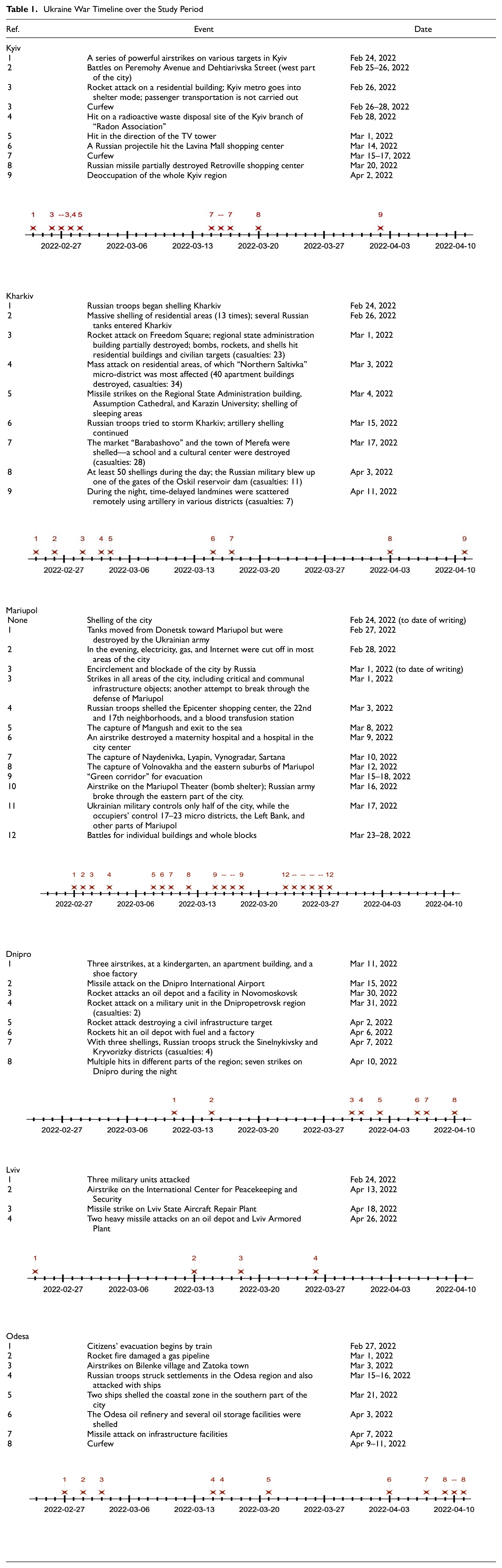
Table 1 lists the timeline of key events in each of the six cities studied in the paper (a more detailed version of which is made available online) ( 30 ). It is formulated via a synthesis of data collected from various sources, including Ukrainian social media platforms, other trusted mass media, socio-political organizations, and official channels of communication of regional military (state) administrations ( 31 – 36 ). The information has been cross-checked for reliability using multiple data sources.

Table 1.

Ukraine War Timeline over the Study Period

Ref.	Event	Date
Kyiv
1	A series of powerful airstrikes on various targets in Kyiv	Feb 24, 2022
2	Battles on Peremohy Avenue and Dehtiarivska Street (west part of the city)	Feb 25–26, 2022
3	Rocket attack on a residential building; Kyiv metro goes into shelter mode; passenger transportation is not carried out	Feb 26, 2022
3	Curfew	Feb 26–28, 2022
4	Hit on a radioactive waste disposal site of the Kyiv branch of “Radon Association”	Feb 28, 2022
5	Hit in the direction of the TV tower	Mar 1, 2022
6	A Russian projectile hit the Lavina Mall shopping center	Mar 14, 2022
7	Curfew	Mar 15–17, 2022
8	Russian missile partially destroyed Retroville shopping center	Mar 20, 2022
9	Deoccupation of the whole Kyiv region	Apr 2, 2022
Kharkiv
1	Russian troops began shelling Kharkiv	Feb 24, 2022
2	Massive shelling of residential areas (13 times); several Russian tanks entered Kharkiv	Feb 26, 2022
3	Rocket attack on Freedom Square; regional state administration building partially destroyed; bombs, rockets, and shells hit residential buildings and civilian targets (casualties: 23)	Mar 1, 2022
4	Mass attack on residential areas, of which “Northern Saltivka” micro-district was most affected (40 apartment buildings destroyed, casualties: 34)	Mar 3, 2022
5	Missile strikes on the Regional State Administration building, Assumption Cathedral, and Karazin University; shelling of sleeping areas	Mar 4, 2022
6	Russian troops tried to storm Kharkiv; artillery shelling continued	Mar 15, 2022
7	The market “Barabashovo” and the town of Merefa were shelled—a school and a cultural center were destroyed (casualties: 28)	Mar 17, 2022
8	At least 50 shellings during the day; the Russian military blew up one of the gates of the Oskil reservoir dam (casualties: 11)	Apr 3, 2022
9	During the night, time-delayed landmines were scattered remotely using artillery in various districts (casualties: 7)	Apr 11, 2022
Mariupol
None	Shelling of the city	Feb 24, 2022 (to date of writing)
1	Tanks moved from Donetsk toward Mariupol but were destroyed by the Ukrainian army	Feb 27, 2022
2	In the evening, electricity, gas, and Internet were cut off in most areas of the city	Feb 28, 2022
3	Encirclement and blockade of the city by Russia	Mar 1, 2022 (to date of writing)
3	Strikes in all areas of the city, including critical and communal infrastructure objects; another attempt to break through the defense of Mariupol	Mar 1, 2022
4	Russian troops shelled the Epicenter shopping center, the 22nd and 17th neighborhoods, and a blood transfusion station	Mar 3, 2022
5	The capture of Mangush and exit to the sea	Mar 8, 2022
6	An airstrike destroyed a maternity hospital and a hospital in the city center	Mar 9, 2022
7	The capture of Naydenivka, Lyapin, Vynogradar, Sartana	Mar 10, 2022
8	The capture of Volnovakha and the eastern suburbs of Mariupol	Mar 12, 2022
9	“Green corridor” for evacuation	Mar 15–18, 2022
10	Airstrike on the Mariupol Theater (bomb shelter); Russian army broke through the eastern part of the city.	Mar 16, 2022
11	Ukrainian military controls only half of the city, while the occupiers' control 17–23 micro districts, the Left Bank, and other parts of Mariupol	Mar 17, 2022
12	Battles for individual buildings and whole blocks	Mar 23–28, 2022
Dnipro
1	Three airstrikes, at a kindergarten, an apartment building, and a shoe factory	Mar 11, 2022
2	Missile attack on the Dnipro International Airport	Mar 15, 2022
3	Rocket attacks an oil depot and a facility in Novomoskovsk	Mar 30, 2022
4	Rocket attack on a military unit in the Dnipropetrovsk region (casualties: 2)	Mar 31, 2022
5	Rocket attack destroying a civil infrastructure target	Apr 2, 2022
6	Rockets hit an oil depot with fuel and a factory	Apr 6, 2022
7	With three shellings, Russian troops struck the Sinelnykivsky and Kryvorizky districts (casualties: 4)	Apr 7, 2022
8	Multiple hits in different parts of the region; seven strikes on Dnipro during the night	Apr 10, 2022
Lviv
1	Three military units attacked	Feb 24, 2022
2	Airstrike on the International Center for Peacekeeping and Security	Apr 13, 2022
3	Missile strike on Lviv State Aircraft Repair Plant	Apr 18, 2022
4	Two heavy missile attacks on an oil depot and Lviv Armored Plant	Apr 26, 2022
Odesa
1	Citizens’ evacuation begins by train	Feb 27, 2022
2	Rocket fire damaged a gas pipeline	Mar 1, 2022
3	Airstrikes on Bilenke village and Zatoka town	Mar 3, 2022
4	Russian troops struck settlements in the Odesa region and also attacked with ships	Mar 15–16, 2022
5	Two ships shelled the coastal zone in the southern part of the city	Mar 21, 2022
6	The Odesa oil refinery and several oil storage facilities were shelled	Apr 3, 2022
7	Missile attack on infrastructure facilities	Apr 7, 2022
8	Curfew	Apr 9–11, 2022

Travel Time Data

Data Collection

We utilize a newly developed OD estimation and network inference methodology for seven city road networks (six urban networks and one highway network in the entire country) in Ukraine ( 25 ). Firstly, we extracted the OpenStreetMap road network data for each network based on the bounding box coordinates. Next, we extracted the link travel time data from TomTom for all the networks. The data collection was done in two periods, that is, February 25–March 16, 2022, and March 25–April 12, 2022. A minimum of three different departure times were set throughout the collection period, that is, morning at 9 a.m., afternoon at 1 p.m., and evening at 5 p.m.

Data Reliability

Although pervasive traffic data are potentially useful in disruptive events, their reliability has not generally been assessed because of the scarcity of such events. For example, using averaged or historical traffic values in the cases that no information sources are detected is a common practice for the navigation providers such as Google and TomTom. Therefore, part of the collected data might only represent routine/average network conditions. Such cases could also be present, specifically in the case study of the Ukraine invasion, with some navigation platforms temporarily turning off the live feature. Therefore, it is also essential to measure data reliability before inferring any travel demand or mobility patterns.

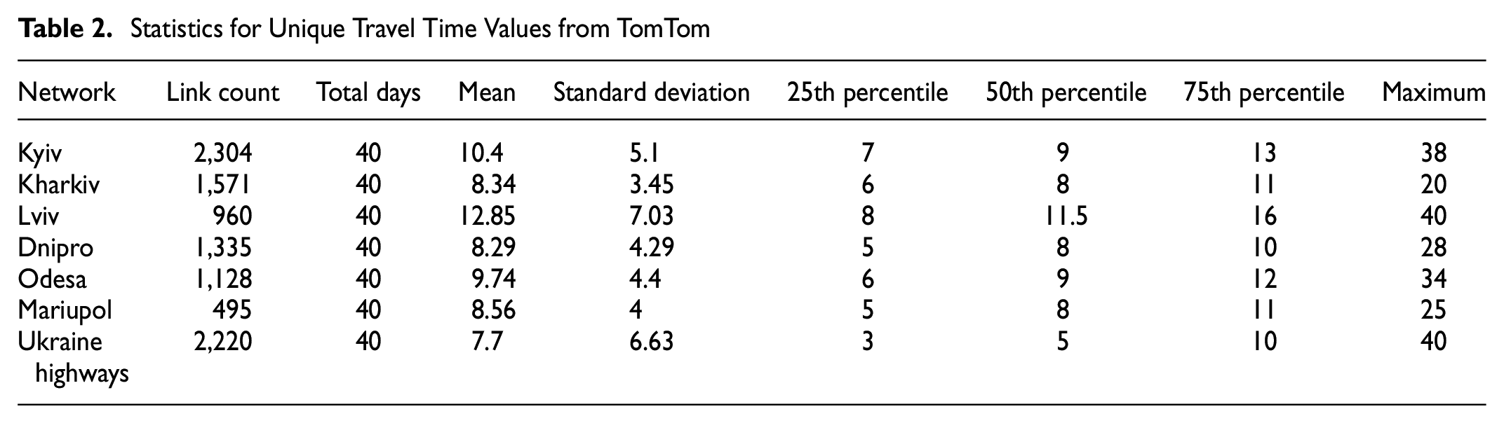
To measure the reliability of the collected data from TomTom, we set the metric to be the frequency of unique link travel time values. We assume that the travel time updates are novel only if they are unique from the other detected times (by up to two decimal places). The analysis is conducted for the six major Ukrainian cities and the Ukraine intercity highway network. It also filters out the shorter length links—that is, shorter than 100 m for all cities and shorter than 500 m for the intercity highway network—which can dilute the findings. Figure 1a shows the histogram of the number of links with their respective unique travel time values observed over the study period (40 days) and Figure 1b provides the probability density functions for all cities to provide a normalized comparison of all cities. Similarly, Table 2 summarizes the related statistics. It is evident that, among all cities, Lviv has the most-frequently updated data, with a mean of 12.85 and 25th and 75th percentile of 8 and 16. All other networks are updated at a mean of 10 or below with relatively lower percentiles values, regardless of their size. Similarly, the Ukraine highway network shows the least update frequencies, with a mean of 7.7 and 75th percentile of only 10. Therefore, for Lviv, the probability density function is also the most well distributed, the Ukraine highway network is the most left skewed, and all other cities show very similar distributions.

Figure 1.

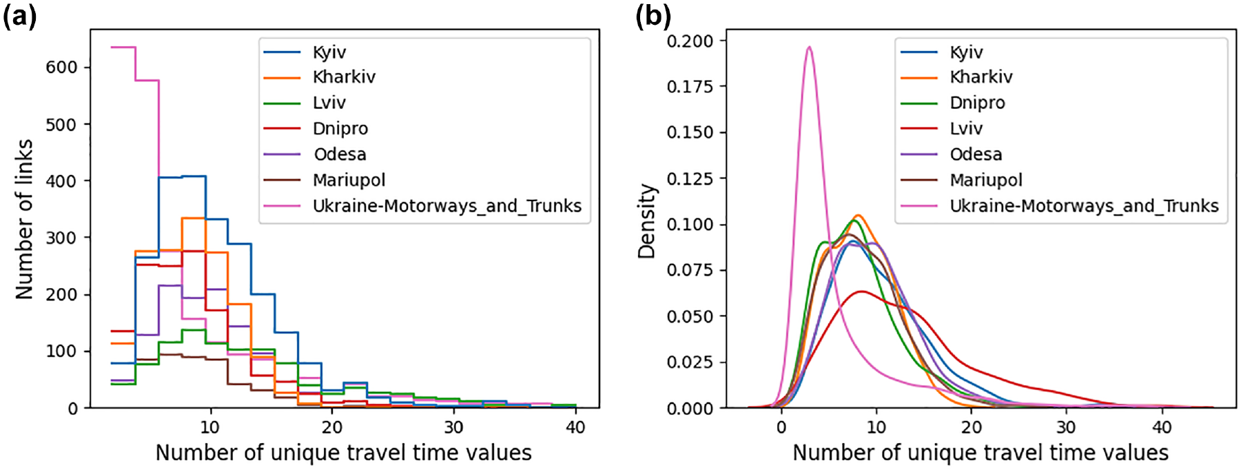
TomTom data reliability plots: (a) histograms of unique link travel times and (b) probability density functions for unique link travel times.

Table 2.

Statistics for Unique Travel Time Values from TomTom

Network	Link count	Total days	Mean	Standard deviation	25th percentile	50th percentile	75th percentile	Maximum
Kyiv	2,304	40	10.4	5.1	7	9	13	38
Kharkiv	1,571	40	8.34	3.45	6	8	11	20
Lviv	960	40	12.85	7.03	8	11.5	16	40
Dnipro	1,335	40	8.29	4.29	5	8	10	28
Odesa	1,128	40	9.74	4.4	6	9	12	34
Mariupol	495	40	8.56	4	5	8	11	25
Ukraine highways	2,220	40	7.7	6.63	3	5	10	40

Analysing Traffic Patterns From Travel Time Data

Link travel times are the best source to directly observe the network traffic patterns; thus, they have been extensively used by practitioners for estimating and predicting travel demand as well as traffic states. Similarly, for disruptive events such as the Russian invasion of Ukraine, link travel times are best suited to help analyze the resulting travel patterns and their relationship with different war disruptions. Therefore, in this section, we utilize the Ukraine travel time dataset (1) to spatially analyze the link travel time variability averaged over the study period and (2) to temporally analyze the link travel time variability and congestion levels throughout the study period. The analysis covers the interstate highway network and six major cities of Ukraine: Kyiv, Kharkiv, Lviv, Dnipro, Odesa, and Mariupol. Note that the two mentioned temporal analyses also relate the observed network disruptions with the war events listed in the section “Ukraine War Locations and Timeline.” Based on the literature review, this appears to be one of the first cases of such analysis of travel patterns for major disruptive human conflict events.

Metrics

Several methods of calculating the travel time variability, such as standard deviation, coefficient of variance (CoV), buffer time index, planning time index, and so forth, have been explored in the literature. The most frequently used method of evaluating the travel time reliability is using the CoV of the travel time, which considers both the variation and the average travel time on a link ( 37 ). It allows demonstrating the normalized variability in travel time.

The following equations show the calculation of coefficients of variance:

$${\mathrm{CoV}}_i^{\mathrm{dW}}=\frac{{\sigma }_i^{\mathrm{dW}}}{{\mu }_i^{\mathrm{dW}}}$$

(1)

$$\mathrm{Co}{V}^{\mathrm{dW}}=\frac{\sum {\mathrm{CoV}}_i^{\mathrm{dW}}}{n}$$

(2)

where

${\mathrm{CoV}}_i^{\mathrm{dW}}$ = the CoV of link i during a moving window of W days for a departure time d,

${\sigma }_i^{\mathrm{dW}}$ = the corresponding standard deviation of travel times for link i during a moving window of W days for a departure time d,

${\mu }_i^{\mathrm{dW}}$ = the corresponding mean of travel times for link i during a moving window of W days for a departure time d,

$i\in I,$ where $I$ is a set of n network links, and

$\mathrm{Co}{V}^{\mathrm{dW}}$ = the average network CoV.

In this study, we considered a moving window of 7 days.

Similarly, many researchers have provided varying definitions and metrics for traffic congestion that are centered on traffic characteristics such as exposure, travel time, delay, speed, volume-to-capacity ratio, level of service, and travel cost ( 38 – 43 ). Each metric has its own merits and demerits. In this study, we consider the ratio of travel time and the free-flow travel time of the link as a measure of congestion level. The following equations show the process of calculating a moving average congestion level for the entire network:

$${\mathrm{CI}}_i^{\mathrm{dx}}=\frac{T_i^{\mathrm{dx}}}{F_i^{\mathrm{dx}}}$$

(3)

$$C{I}^{\mathrm{dx}}=\frac{\sum {\mathrm{CI}}_i^{\mathrm{dx}}}{n}$$

(4)

where

${\mathrm{CI}}_i^{\mathrm{dx}}$ = the congestion index of link i at a departure time of d on a specific day x,

$T_i^{\mathrm{dx}}$ = the corresponding travel time for link i at a departure time of d on a specific day x,

$F_i^{\mathrm{dx}}$ = the corresponding free-flow travel time for link i at a departure time of d on a specific day x.

$C{I}^{\mathrm{dx}}$ = the average network congestion level, and

n = the number of links.

Spatial Analysis of Link Travel Time Variability

Figure 2 spatially visualizes the CoV metric of travel time for each network link over the whole study period (morning departure time). The metric is scaled using a hue scale that ranges from dark blue depicting lower variability, to dark red depicting higher variability. While analyzing the figure, it is evident that, for all cities, links in the outer city regions show much higher variability than the inner (or city center) regions. The resulting patterns can be arguably interpreted as showing that, since since inner city regions are densely populated, have high shares of regular commutes, and are prone to more frequent war incidents (e.g., shelling, missile attacks, or occupation attempts), they might result in lesser, but consistent, traffic congestions. In comparison, the higher variability and disruption in the outer region are because of factors such as irregular blockage/availability and irregular collective migration patterns to and from the city affected by the war situations.

Figure 2.

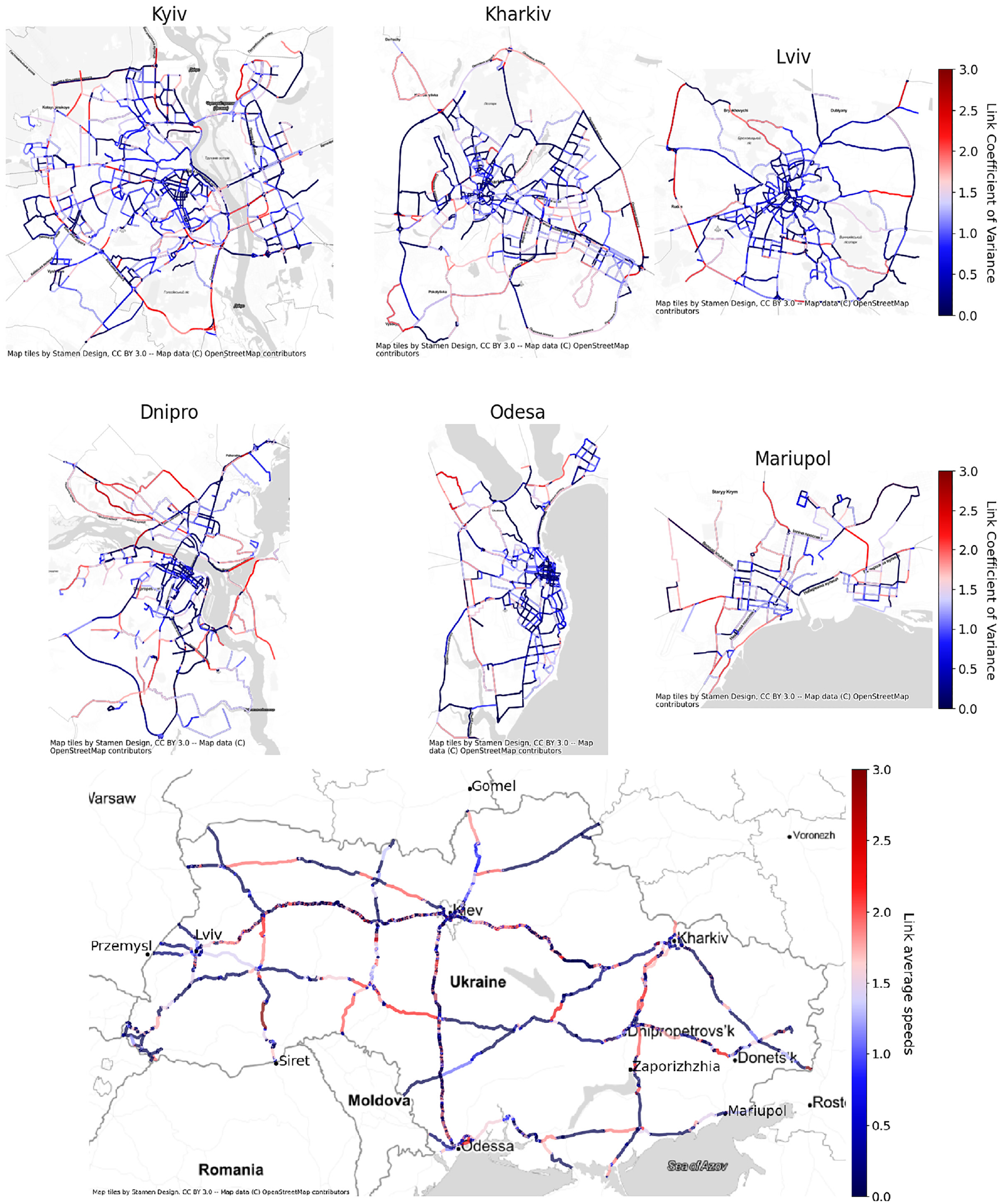
Hue maps for link coefficient of variance (CoV) over the whole study period.

Further about individual cities: the three cities of Kyiv, Kharkiv, and Mariupol were under attack from the first day of the war (see Table 1), and therefore its effect is evident in Figure 2, where the hue maps of all three cities show overall higher variability in link travel times compared with other cities (showing lighter blue tone to red tone). Note that, while comparing these three cities, the city of Mariupol, which has been most affected by the Russian invasion, does show the highest variability; Kyiv, having strong defense capture, shows the least variability inside the city; and Kharkiv shows higher variability in the north, south, and southeast regions which contain radial links that connect the city toward Russia, Russian occupied territories, and Dnipro.

Similarly, the other three cities of Lviv, Dnipro, and Odesa show similar patterns, where most regions show the least variability while some show very high travel time variability. Since Dnipro, together with Zaporizhzhia, were the cities where evacuation vehicles arrived from occupied territories, almost all radial links for accessing the city depict high variability; whereas Lviv, being the city least directly affected by Russian attacks, shows the least variability. For Lviv, although it is mentioned that it acted as the logistic and humanitarian hub with millions of people from the whole country consistently arriving in the city, the east city links depict a rather mild variability compared with Dnipro, whereas the west side links do depict very high variability.

Finally, concerning the travel patterns in Ukraine’s intercity highway network, the effects of the Ukraine war are evident. All migration routes, including the westside highway network of Ukraine that connects to Lviv and Europe and the highways to Moldova, show much higher travel time variability. Similarly, the route from Dnipro to Kharkiv also depicts high variability since the city acts as the destination for evacuation vehicles. The highways connecting Kyiv from north (Gomel) and northwest, and the highway connecting Kharkiv to north (Russia) were under the Russian occupation and also show high variability because of Russian military movements. The highway connecting Kyiv to western region was blocked by Russian by destroying a large bridge en-route. Other access routes to Kyiv and Kharkiv also show a mix of high and low variability links (maybe because of blockages/destroyed bridges, limited data observability, etc.), depicting varying traffic congestion patterns.

Temporal Analysis of Travel Times Variability and Network Congestion Levels

This section provides a temporal analysis of the effects of Ukraine war events using link travel time variability and network congestion levels. First, Figure 3 plots the temporal travel time variability using the network-wide average of the 7-day moving CoV (Equation 2) for link travel times at three departure times. The metric helps in understanding the moving temporal variability in travel time uncertainty over a 1-week period. Then, Figure 4 plots the 7-day moving network-averaged link congestion indexes (Equation 4). Each subplot from both figures visualizes three different time-of-day results from the morning, evening, and whole-day link travel times for each of the six cities focused on in this study. To help interpret the plot trends, we also label the reference numbers of the key war events that occurred in each city during the study period (listed in Table 1). Below, we analyze the results from each city separately, considering its situation and the timeline of events mentioned in section “Timeline.”

Figure 3.

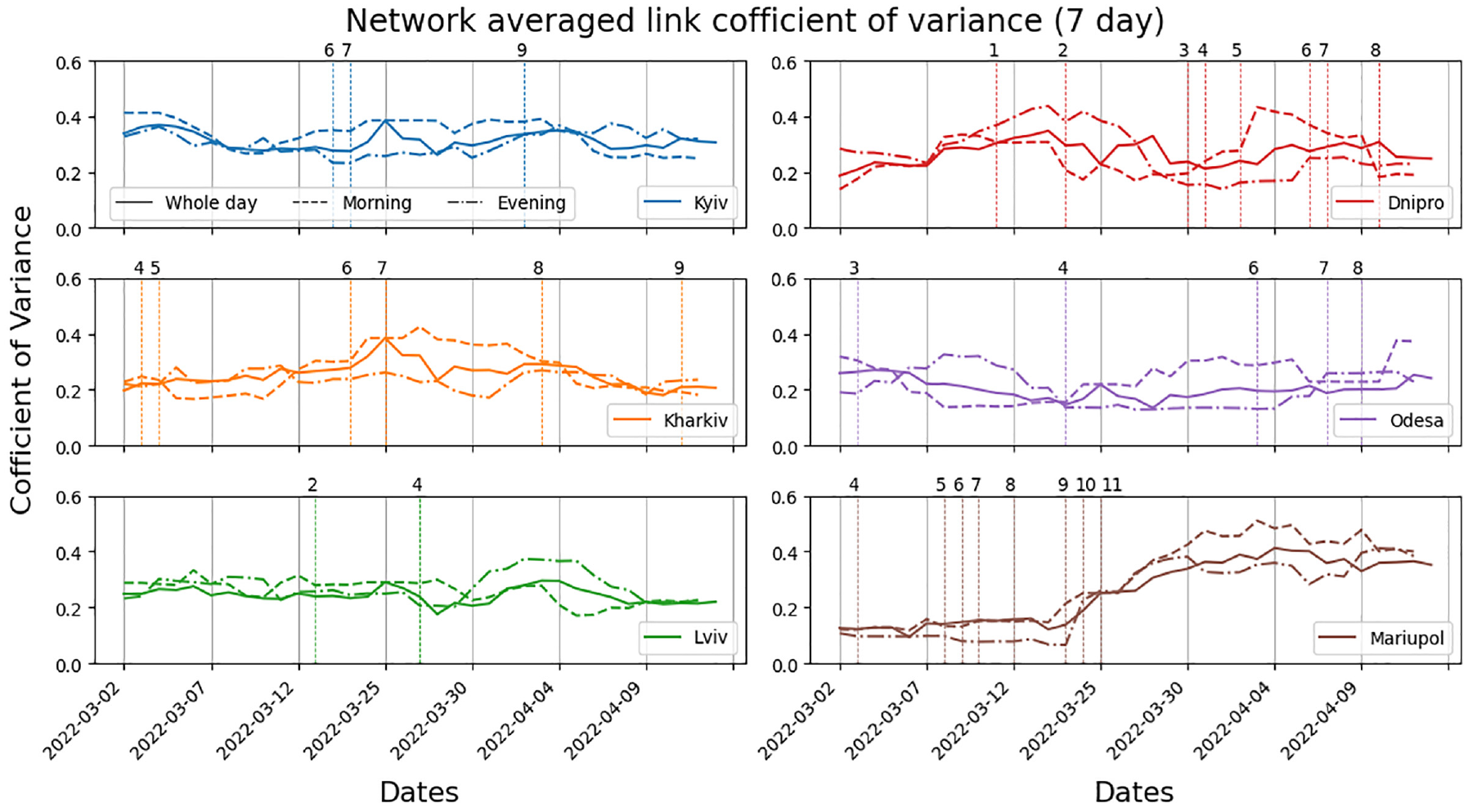
Network averaged link coefficient of variance (CoV) for travel times (7-day moving).

Figure 4.

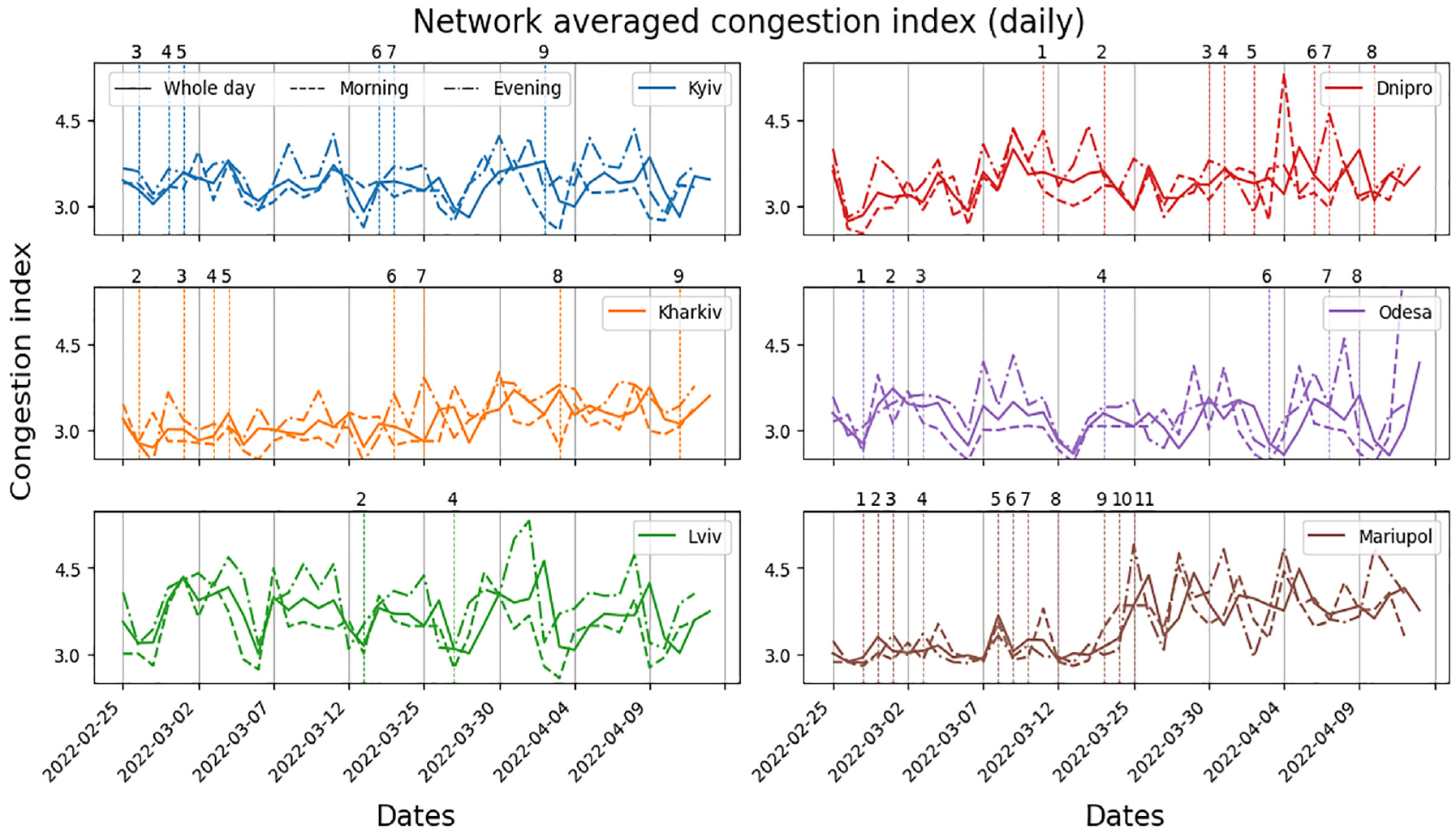
Network averaged congestion index.

Kyiv: For Kyiv, two prominent trends are present in travel time variability (Figure 3): 1) the times after curfews (Event 3 [February 26–28, 2022] and Event 7 [March 15–17, 2022]) show a clear increase in travel time variability and 2) two periods of time show a clear (decreasing) trend of calmness and regularity in congestion patterns, one between March 1 and March 14, 2022, in which less severe attacks on Kyiv are recorded, and the other around the de-occupation time of Kyiv region (April 2, 2022) (decreasing trend for the morning and whole-day travel time variability). Likewise, the only prominent trend visible in Figure 4 is around the Kyiv region de-occupation (Event 9 [April 2, 2022]), where the morning congestion levels continuously decrease until the event weekend (i.e., the calmest morning of the study period), while the whole-day congestion levels stay low for the next few days.

Kharkiv: While Table 1 only mentions a few key war events for Kharkiv, it was under consistent attack from Russia and shows a slight but continuous increasing trend in travel time variability (Figure 3) until Event 7 (multiple attacks from Russian troops with up to 28 civilian casualties). However, after Event 7, while the morning travel time variability remains rather high, overall, the travel time variability shows a continuous decreasing trend toward calmness and regularity in congestion patterns because of less severe attacks.

Lviv: Since Lviv is located in west Ukraine, farthest from Russia or its occupied territories, it has much fewer severe events and shows consistent travel time variability (Figure 3) apart in one period between March 26 and April 10, 2022. During this period, both travel time variability and congestion levels show higher trends for the evening and whole-day times. These trends can be explained by: 1) the Event 4 (two large missile attacks on Lviv) occurring on March 26, 2022, after which the higher uncertainty in travel time and congestion levels can be seen and 2) the de-occupation of the Kyiv region (around April 2, 2022), causing the return of people from west of Ukraine and abroad, many of whom went through Lviv, as it acted as the major logistic and humanitarian hub.

Mariupol: Mariupol has been one of the prime occupation targets for Russia to create an overland corridor to occupied Crimea. Therefore, the city was practically under siege within the first week (February 28, 2022, saw the utilities cut off in most areas, and by March 1, 2022, Russia had blocked the city). The situation changed with the opening of a “green corridor” for evacuation (Event 9, March 15–18, 2022), during which the city showed a steep increase in travel time variability and congestion levels. Further, the occupation battles continue to occur (Event 12) between March 23 and 28, 2022, maintaining similar increasing trends in both metrics. It is also essential to signify that by March 17, 2022 (Event 11), already half of the city was under Russian occupation, which by March 28, 2022 (end of Event 12) increased to almost the whole city. Therefore, the increased variability trends in travel times and congestion levels after March 28, 2022, occurred under Russian occupation.

Dnipro: Apart from being constantly under attack, Dnipro also acted as an evacuation hub and home to thousands displaced by the war (being located near Kharkiv and Mariupol). Therefore, much of the variability in both travel times and congestion levels can be referred to the general war timeline. Overall, each of the two data collection periods shows prominent travel time variability peaks (Figure 3), that is, March 2–16 and March 27–April 12, 2022. The variability trends during the first peak period can be attributed to war events in Kyiv, Kharkiv, and Mariupol, in which the evening times consistently show high values for both metrics. Similarly, the variability trends during the second peak period are mainly significant for morning time and can be attributed to Events 3–5, that is, regular rocket attacks in Dnipro between (March 30–April 2, 2022). Note that the time frame also coincides with the de-occupation of the Kyiv region.

Odesa: For Odesa, multiple prominent variability trends are seen in link travel times and network congestion levels. First, both metrics show rapid increases after the curfew period from April 9 to 11, 2022, where the morning time congestion levels see a very sharp rise. Then, while the travel time variability calms until March 15, 2022, the large set of attacks by Russia (Event 5) on March 15 and 16, 2022, retriggers its increase. Similarly, Figure 4 shows three different sets of congestion level peaks for morning or evening times, some of which can be related to the attacks on April 3 and 7, 2022 (Events 6 and 7), which seem to trigger a sharp rise in congestion levels for the next day.

Overall, to conclude, the analysis does depict clear impacts and correlation of war events with travel time variability and congestion index for all cities. For example, the cities of Kyiv and Mariupol show direct impacts of Russian invasion and occupation/de-occupation events, while the cities of Kharkiv, Dnipro, and Odesa also show significant changes in travel time patterns after Russian attacks. Moreover, the return trend of calmness and regularity in congestion patterns after abrupt variability caused by Russian attacks is also evident in many cities (i.e., Kyiv, Kharkiv, Dnipro, and Odesa).

Analyzing Travel Patterns By OD Demand Estimation

Historically, researchers and practitioners depended on OD demand data acquired through household travel surveys (HTS) ( 44 ). These surveys are conducted as one-time events every few years, and are labor intensive, expensive, and frequently out of date ( 23 ). The HTS data are useful in long-term planning models, but they are not suitable for day-to-day traffic analysis or developing operational plans during disruptive events. Many investigations made use of non-traditional data sources such as loop detectors, Bluetooth, and registration plates ( 25 ). However, they lack spatial coverage, are time-consuming to collect, costly to set up and operate, and are also not suitable for rapid and automated planning in conflict circumstances where data collecting and the processing time are critical. Therefore, alternative methods are essential.

Trip Table Estimation

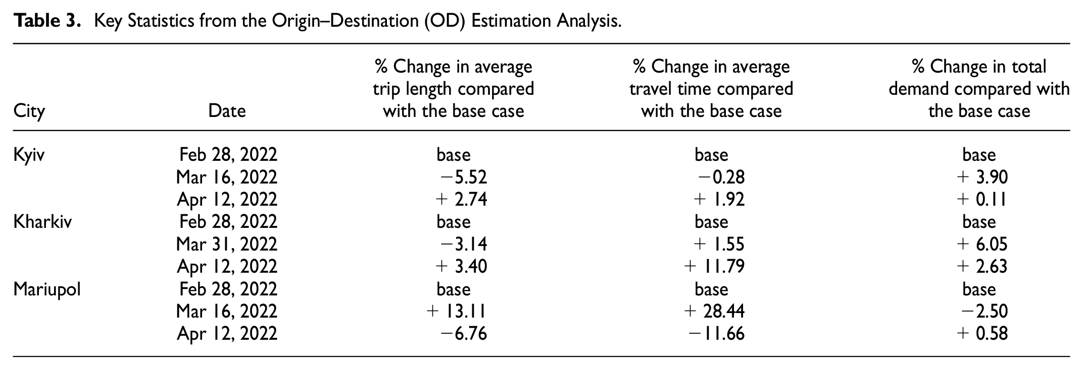
We used Rapidex, a recently developed methodology that utilizes crowd-sourced travel time data to estimate OD trip tables, zonal structure, and network supply ( 25 ). Specifically, we estimated the trip tables through travel time data collected through TomTom on three different days. These three days correspond to: (1) the start of the invasion, (2) an intermediate time or critical event, and (3) the last day of the study period. We confine our investigation to three cities (Kyiv, Kharkiv, and Mariupol) and three specific dates, because of space constraints. We used a server with 40 cores, 3.1 GHz processing speed and a memory of 512 GB. We first defined the network zoning configuration, including the number of zones and centroids. Then, the methodology utilizes link travel times and runs a genetic algorithm technique to derive OD matrices. These matrices were then used as source data for a network modeling process to estimate key metrics such as travel times, trip length, and congestion levels. This OD estimation technique can be seen as an advancement on past methods that rely on extensive and costly surveying of household travel behaviour, thus providing a viable option for developing countries facing data poverty challenges ( 18 ). Interested readers are recommended to refer Waller et al. for more details on the OD estimation process ( 25 ). Table 3 shows the percentage changes in key metrics compared with the base day, that is, February 28, 2022, for each of the three cities.

Table 3.

Key Statistics from the Origin–Destination (OD) Estimation Analysis.

City	Date	% Change in average trip length compared with the base case	% Change in average travel time compared with the base case	% Change in total demand compared with the base case
Kyiv	Feb 28, 2022	base	base	base
	Mar 16, 2022	−5.52	−0.28	+3.90
	Apr 12, 2022	+2.74	+1.92	+0.11
Kharkiv	Feb 28, 2022	base	base	base
	Mar 31, 2022	−3.14	+1.55	+6.05
	Apr 12, 2022	+3.40	+11.79	+2.63
Mariupol	Feb 28, 2022	base	base	base
	Mar 16, 2022	+13.11	+28.44	−2.50
	Apr 12, 2022	−6.76	−11.66	+0.58

Zone production levels and destination congestion index

To further examine the travel behavior patterns during the invasion of Ukraine, this section analyzes the zone-averaged congestion indices and demand generation metrics for the three cities of Kyiv, Kharkiv, and Mariupol. First, Figure 5 spatially visualizes the zonal destination congestion index to examine zone (attraction) impedance or accessibility, then Figure 6 spatially visualizes the zone production percentages to examine the demand contribution patterns. Below, we discuss the analysis of each city separately:

• Kyiv: By February 28, 2022, Kyiv had experienced a series of airstrikes and rockets, a curfew, the Kyiv metro going into shelter mode, and the Russian military occupation nearly as far as the town Bucha, that is, northwest of Kyiv. However, for February 28, 2022, both metrics in Figures 5 and 6 mostly show normality, with high levels in the city’s dense central area and low levels in almost all outer city regions. Most of the patterns continue for March 16 and April 12, 2022, because of Kyiv’s strong defense forces thwarting all occupation attacks by Russia. However, two prominent trends are evident from both figures. First, a steep rise in congestion levels and trip productions are seen in the west city region on March 16, 2022, which indicates the advancements of the Russian military that, by that time, had occupied the outskirt regions (including Bucha) in the northwest and west of Kyiv, resulting in people migrating toward Kyiv and increasing congestion levels in the west. Later, by April 12, 2022, this trend is reversed back, because of the de-occupation of Kyiv. Then, the other trend of consistently higher levels of congestion in the southwest city area is also visible. The region mainly contains rural highways which connect Kyiv to the southwestern region, and the increase in congestion levels is arguably because of the network serving as a migration route, since one of the two major highways connecting Kyiv to west Ukraine was occupied by Russia (the northwestern highway through Bucha) while the other was disconnected by destroying a large bridge (the western highway).

• Kharkiv: Similar to Kyiv, by February 28, 2022, Kharkiv had already experienced many attacks from the Russian military, including tens of shelling attacks and even several Russian tanks entering the city (Events 1 and 2). However, none of the Kharkiv city areas came under Russian occupation throughout the study period. Therefore, apart from the eastern, southeastern, and northwestern city areas, the patterns for zone productions and destination congestion index are rather consistent, that is, high levels in the densely populated city central area and relatively lower levels in the outer city areas. The eastern city area of Saltivka saw consistent mass attacks by Russia (Table 1) and evidently saw a distributed increase in congestion levels, which, interestingly, also does not translate into an increase in production for that region ( 24 ). A similar trend is also seen for the northwestern suburban area of Derhachi, which also shows a sharp rise in congestion levels, but only for the April 12, 2022, plots without any increase in trip productions. This trend also results from the consistent shelling by Russian troops on Derhachi between April 9 and 11, 2022 ( 24 ). Finally, the southeastern (industrial) region of Kharkiv, which was also heavily shelled by Russian tanks and artillery on April 10, 2022, also shows similar patterns of increase in congestion levels.

• Mariupol: Mariupol city is administratively divided into four districts: “Kalmiuskyi” (northern city area), “Livoberezhnyi” (left bank or southeastern city area), “Prymorskyi” (southwestern city area containing the seaport), and “Tsentralnyi” (the central city area in the middle-west). February 28, 2022, was a day before the blockade of Mariupol city by Russia. Before that time, the city did not suffer many Russian attacks; therefore, the plots show close-to-routine travel patterns, that is, in Figure 5, the central city area and the port area show a higher destination congestion index, and in Figure 6, the central city area, port area, and the west part of the left bank region show high production rates.

Then, March 16, 2022, was the second day of the 3-day green evacuation corridor period intended to allow the citizens to evacuate the city. However, for congestion levels, only a slight increase is seen in the western and southwestern city regions, whereas the metric is unchanged for the northern city region, both of which should generally be considered evacuation routes. Further, on this day, the Russian army broke through the eastern part of the city (Event 10), an event whose effect is visible because the congestion index levels show the activity with much higher levels in the left bank area. Concerning production rates, they significantly reduce for the central city area (less-to-no routine activities), slightly increase for the port (possible military movement), and remain similar but considerably distributed in the left bank and northeast regions (indicating Russian troop movement).

Figure 5.

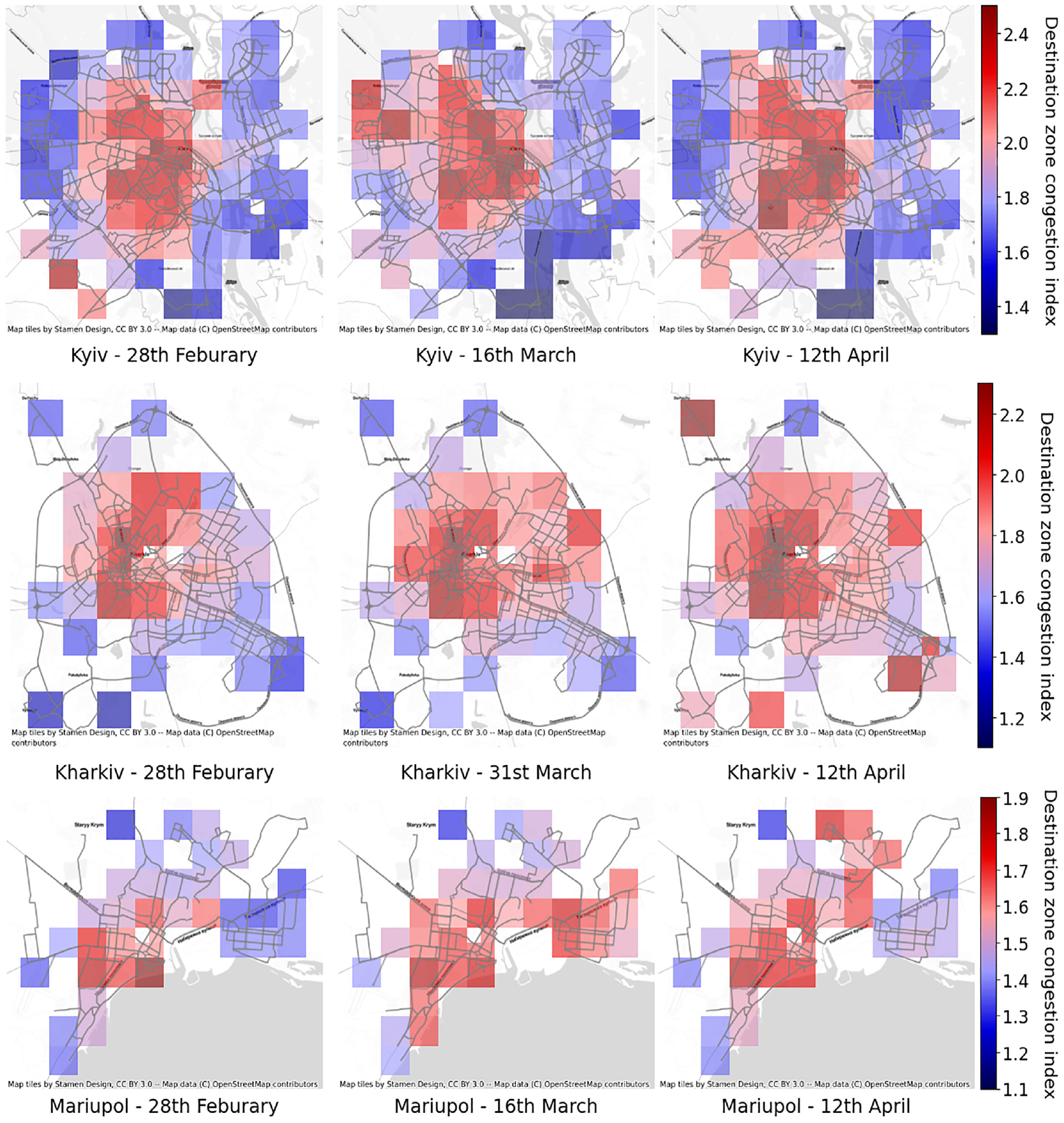
Hue maps of average congestion index for zones as the destination (various dates in 2022).

Figure 6.

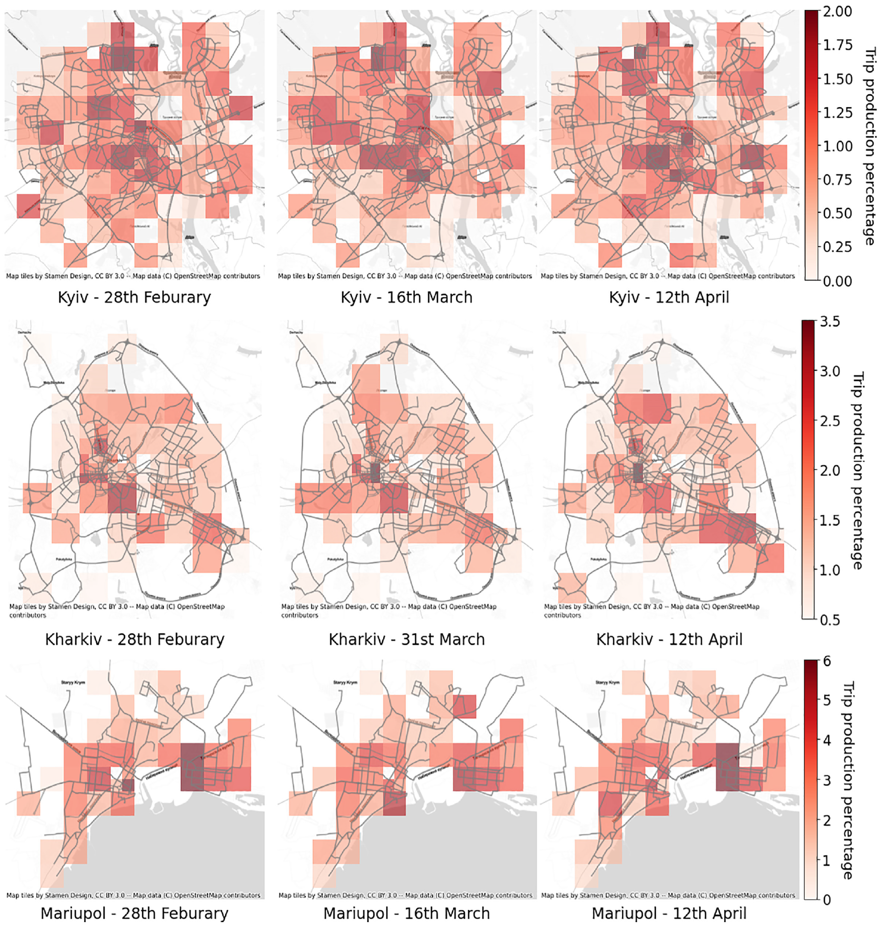
Hue maps of percentage shares of zone productions (various dates in 2022).

Finally, by April 12, 2022, most of the Mariupol city was under Russian occupation, and the zone destination congestion index levels were, again, back to lower level for the left bank, similar (distributed) for the central city, and much higher for the northern city area. Note that the congestion patterns do have a significant change reflecting Russian military activities in the city, since most Ukrainian soldiers and many civilians were (by then) hiding in Azovstal plant (east of the port).

Conclusions

Disruptive events such as a national invasion are rare and, therefore, disruption-induced travel patterns are not commonly analyzed. The presented research utilized crowd-sourced pervasive traffic data from TomTom to evaluate traffic patterns, estimate network supply, and model OD traffic demand during the ongoing Ukrainian conflict as it unfolded. The analysis demonstrated the utility of such data to determine and relate the impacts on travel patterns during such a major disruptive event.

Specifically, the research utilized and extended a recently developed demand/network estimation methodology to model and analyze travel impacts during the Ukraine invasion. The methodology enables researchers to quickly compare various policies and events by evaluating the trip tables across various networks and help understand aggregate time-period-based demand changes, or analyze the impacts of network and demand changes on critical performance metrics. Critically, the approach differs from basic analytics in that a network traffic assignment model is created, which allows comparative analysis within a planning approach. It should be noted, however, that the model produces highly aggregate outputs but is useful in situations where more traditional modeling solutions are not possible or prohibitive in relation to resourcing, particularly in rapidly evolving large-scale human conflict.

To conduct the study and relate the travel analysis, 51 key war event periods were synthesized (Table 1). For absolute temporal travel time variability, Mariupol shows the highest level at 0.5 under Russian occupation. Kyiv, Kharkiv, and Dnipro show up to a value of 0.4, whereas, for the relative increase in variability, Mariupol, Dnipro, and Kharkiv show up to 200%, 135%, and 100% change, respectively, during the study period. Finally, for the three most-attacked cities of Kyiv, Kharkiv, and Mariupol, the invasion events triggered up to 50%, 55%, and 30% increase in congestion levels and up to 200%, 150%, and 300% increase in demand productions, respectively.

One limitation of the current study is that, because of the damage to the road network, parts of the network could be impaired. While the presented findings align at the highly aggregated level of analysis used in this study, future research will endeavour to model the destructive variant of the network design problem where system capacity will join the OD demand values within the evolutionary algorithm variable set.

In relation to future research, the analysis presented in this paper highlights the necessity for tailored forms of travel demand management in ongoing research. Ensuring human safety, while adapting to uncertain system capacity, is one defining characteristic of human conflict scenarios. As a result, the travel management of safety-oriented curfews, work-at-home capability, rapidly adaptive public transport, walking, and cycling take on even greater importance under the examined conditions.