Sage Journals: Discover world-class research

Abstract

Global System for Mobile Communications (GSM) data provides valuable insights into travel demand patterns by capturing people's consecutive locations. A major challenge, however, is how the polling interval (PI; the time between consecutive location updates) affects the accuracy in reconstructing the spatio-temporal travel patterns. Longer PIs will lead to lower accuracy and may even miss shorter activities or trips when not properly accounted for. In this paper, we analyze the effects of the PI on the ability to reconstruct an origin–destination (OD) matrix. We also propose and validate a new data-driven method that improves accuracy in case of longer PIs. The new method first learns temporal patterns in activities and trips, based on travel diaries, that are then used to infer activity-travel patterns from the (sparse) GSM traces. Both steps are data-driven thus avoiding any a priori (behavioral, temporal) assumptions. To validate the method we use synthetic data generated from a calibrated agent-based transport model. This gives us ground-truth OD patterns and full experimental control. The analysis results show that with our method it is possible to reliably reconstruct OD matrices even from very small data samples (i.e., travel diaries from a small segment of the population) that contain as little as 1% of the population’s movements. This is promising for real-life applications where the amount of empirical data is also limited.

Keywords

data analytics machine learning (artificial intelligence)mobility passive data supervised learning telecommuting transportation planning analysis and application

The design of transport infrastructure, services, policies, and technology all starts with an understanding of travel demand. Travel demand relates to people’s spatial and temporal patterns of activity locations and associated trips from one location to the next, and are commonly aggregated into origin–destination (OD) matrices. One data source in this is Global System for Mobile Communications (GSM) data as they allow people to be traced (carrying the mobile phone). The time between consecutive location updates is called polling interval (PI), and evidently affects the accuracy with which we can reconstruct people’s spatio-temporal travel patterns.

Traditionally, traffic planners use direct methods, including roadside and household surveys, conducted every 5 to 10 years ( 1 ) for estimating the OD matrix. While these methods are making essential contributions to the traffic demand field, exclusively using survey data makes the estimations liable to sampling bias and reporting errors ( 2 – 4 ) because travel surveys provide a high level of detail (LOD) as regards activity and movement behavior with minimal sampling ratios. Conversley, mobile phones have generated a wealth of low-cost GSM data on people’s movements. These movement traces are often of reasonable sample size but contain (much) less detail than survey data. Generally, GSM data contain discretized traces of users without precise indicators of time and location of the underlying activities or activity types. Therefore, before being used to estimate the OD matrix, the data need to be analyzed.Combining travel diaries in such GSM analyses could potentially lead to the best of both worlds; that is, the high sampling ratio of mobile phone data combined with the high LOD (concerning spatial and activity patterns) in travel diaries.

Fundamentally, two types of synthetic and real-world data sets are used in demand estimation research. Real-world GSM data sets can offer voluminous information about millions of mobile phone users. However, the problem with them is the privacy issue and difficulty of carrying out reliability and validation experiments. In fact, in the early analysis phase of research, using synthetic data for assisting in the operational tests and evaluation has been strongly advocated ( 5 ). Conducting experiments using such data helps us to evaluate the effects of various potential components in our models. Therefore, in this paper we used synthetic (travel diary and GSM) data to validate our methods. Moreover, it enabled us to produce many ground-truth training sets for statistical learning and reliability testing.

Our method addresses some key questions concerning the accuracy and robustness of OD matrices estimated from GSM data related to the temporal discretization. Clearly, such discretization errors could be reduced by choosing smaller PIs between records. However, this is often not possible since, by their very nature, GSM records are spatially coarse and temporally infrequent (e.g., Becker et al. [ 6 ], Burkhard et al. [ 7 ], and Chen et al. [ 8 ]). To date, few studies have investigated the relationship between GSM quality and mobility pattern detection (e.g., Calabrese et al. [ 9 ] and Chen et al. [ 10 ]). To the best of our knowledge, no study has looked specifically at the effects of GSM data temporal frequency on the estimated OD matrix. This paper is the first to examine these effects. To do this, we quantify the temporal quality of the data using PI, defined as the time interval between consecutive records, where a record is an update on the current location of the mobile device. (Note that the inverse of the PI is referred to as polling frequency.)

There are two consequences to the temporal record of events is being descretized (with the PI). The first effect is that the recorded start and end times of each underlying event (an activity or travel between activities) occur later than the actual start and end times. This discretization error can vary from zero to the PI value. For instance, if we poll the user epsilon before the actual event time, the interpreted time is about one PI later.

To illustrate, Figure 1a shows several GSM records of a user. Note that while the reported locations in the empirical GSM data belong to the antenna that receives the cell phone signal, in this example, we assume that these records are the user’s exact locations. The spatial changes and errors could be investigated in separate research—here, we focus on temporal effects only. Therefore, the person has been observed in five locations (Figure 1b) named {A, B, C, D, E} with a constant PI of 15 min. However, the actual travel diary implies that only in two of the reported locations (A and D) activities occur (work and home); thus, understanding whether the user is traveling or staying (engaging in an activity) in each record requires developing a separate procedure. To decide on the event type (travel or stay), one could for instance use each event’s starting time and duration. Moreover, based on Figure 1a, the user was observed in A from 15:35 to 16:20, but the actual traces imply that the user stayed at the mentioned location from 15:23 to 16:15 to work; therefore, owing to time discretization, delay in observing the start and end of each event is inevitable. How PIs affect the resulted OD matrix (under different conditions) is part of this study.

Figure 1.

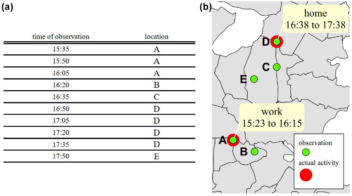
An example of the Global System for Mobile Communications (GSM) records of a user: (a) a prototype of GSM traces and (b) visual representation of traces in (a).

The second—and related—consequence of time discretization is the discrepancy between observed and actual activity (or travel) duration. For instance, in Figure 1, the perceived duration of A is 45 min; whereas, the actual duration is 52 min. This duration discretization error ranges from -PI to PI. In fact, we may even lose a fraction of OD trips (i.e., observed with zero duration) because the data might not capture specific trips with duration less than the PI. For example, activities that last less than one minute could easily be missed from the GSM data with high PI. In many cases, detecting such short-time activities is not very useful from a travel demand perspective. However, if activities are longer (e.g., more than 15 min), it might be insightful to configure them. Consider for example three activity categories—home, work, and other—representing staying at home, working, and engaging in other types of activities, respectively. One could argue that for OD matrix estimation, the distinction between stay (on a specific location) and travel (between locations) is sufficient. Home and work are major activities from a traffic planner’s perspective since they account for a large part of travel diaries. Additionally, they often have aggregated daily durations of a couple of hours, making them more likely to be captured, even with very coarse PIs. However, other encompass all activities made for less common purposes, such as shopping, socializing, and health. The duration of these is usually much shorter than home and work. The maximum PI (for having cell phone reception in case of no network connection) adopted by the telecommunication company is about 2 h. Consequently, there are interactions between the mix of activity durations and PIs, whose effects on the reconstructed OD matrix are not fully understood. It is our aim to gain a better understanding of how the reconstructed OD matrix deteriorates by testing a range of duration–PI combinations (from 1 min to 2 h).

To this end, our approach is threefold.

Pre-processing and ground-truth analysis: First, we generate synthetic GSM data directly from a detailed set of ground-truth travel diaries. Furthermore, to train our GSM interpretation method (for event-activity type detection), called the kernel-based approach (KA), we select a random 1% sub-sample from the ground-truth travel diaries.

Developing and applying KA and OD matrix determination: Second, we develop and validate the KA algorithm by which we reconstruct the travel diary of each person for determining the OD matrix from the interpreted GSM data.

Comparison of OD matrices: Third, we compare the reconstructed and actual OD matrices derived from the interpreted GSM data and ground-truth, respectively, where we use multiple evaluation metrics.

This way, our analysis studies the mixed effect of the PI and temporal criterion. Our method adopts this interaction (derived from the training data) to discern activities from trips on the reconstructed OD matrix. Therefore, our results show the causes that affect the accuracy and robustness of the estimated OD matrix using GSM traces.

In this research, the following contributions are made:

We propose and evaluate a data-driven method for interpreting GSM data, which does not rely on a priori assumptions of activity-travel behavior, and therefore is applicable for both synthetic-experimental analyses (as in this paper) and empirical-practical implementation.

We show that even a small portion of the population could train our method for location-activity type detection of GSM records. This method could further be trained when more observations are available.

We provide an overview of the effect of the underlying PI on the resulting OD matrix. Our analysis results also imply that the shorter the activity duration, the less its possibility to be identified correctly.

We show when randomness in the OD matrices spike relatively to how frequently we poll the users.

As a case study, the research is performed with the data of the Amsterdam region in The Netherlands. We assume to have GSM data of a given population (i.e., we do not deal with the second-part problem of scaling from GSM sample toward full population) as well as a limited amount of travel dairies (i.e., 1% of the given population).

The next section of this paper explains fundamental characteristics of GSM data that need to be accounted for. That is followed by a section that describes the research data and the implemented method. Next, we evaluate the proposed method, present the results of applying the method on the GSM data for reconstructing the OD matrix, and compare it with the ground-truth OD matrix. The paper concludes with a conclusion and outlook section.

GSM Data in General and as Used in This Study

Basically, three main types of GSM data are generated by telecommunication companies:

The first type is call detail record (CDR), which constitutes a majority of GSM data in transport research (e.g., Calabrese et al. [ 9 ] and Chen et al. [ 10 ]). It includes event-based history information on the communication of a specific device, which consists of calls, SMS (short message service), internet connections. CDRs consist of the timestamp, call duration, type of events (voice call, SMS, data), and the cell’s code in which the event occurs. Consequently, recording phone positions is dependent on the users’ communication behavior. Therefore, we need to assume on how to generate synthetic CDR. For instance, a random communication rate derived from a Poisson distribution between a minimum and maximum rate can be assumed for each user. A more mature and complex scenario uses discrete choice theory, which is based on utility maximization; that is, it couples agent’s decisions to attributes of the alternatives and agent’s environment.

The second type is named signaling data which informs us of the location area (LA) of the mobile phone on a permanent basis. Nonetheless, its spatial resolution is much lower than CDR because each LA includes more than a hundred base stations ( 11 ). Therefore, this type of data does not seem suitable for demand estimation and activity analysis for transportation purposes.

The third type which is called periodic location update (PLU) contains anonymous user ID code, time of the day, and location coordinates. Unlike CDR, PLU does not involve mobile phone users for storing their records. In fact, the GSM operating system decides on when to collect all users’ data. Additionally, the spatial resolution is the same as CDR. Moreover, the PI is constant among all users independently from their behaviors. Thus, the random errors of the data has been partially eradicated owing to the fixed interval of records. As a result, activity locations would be detected efficiently and by shorter data collection time. However, compared to CDR, accessing such data is an arduous task. Nonetheless, some research has already used them in mobility demand estimation (e.g., Zhang et al. [ 12 ]).

In this study, we used PLU instead of CDR because it does not rely on a priori assumptions between GSM data events and activity-travel behavior (which may otherwise introduce behavioral biases if not adequately addressed). Indeed PLU is therefore applicable for both synthetic-experimental analyses (as in this paper) and empirical-practical implementation.

As all types of GSM data capture the movement of vehicles and people, they could be used in estimating the travel patterns. However, one needs to deal with the new challenges of developing, and validating of models adopted for estimating the OD matrix. In fact, despite the great opportunity of using GSM traces for OD matrix estimation, several drawbacks cause obstacles when it comes to practice:

Mobile phone data only observe the user’s presence at a certain point in time in a particular mobile phone cell. Whether the person was traveling then or attending an activity cannot be directly concluded ( 5 ). Therefore, one must interpret the GSM traces to reconstruct the travel patterns. Several previous researchers have specified a certain duration (or speed) to make a distinction between stay and pass-by locations in the GSM records (e.g., Iqbal et al. [ 13 ], Alexander et al. [ 14 ], and Demissie et al. [ 15 ]). For instance, Iqbal et al. ( 13 ), Alexander et al. ( 14 ), and Demissie et al. ( 15 ) assumed that a trip is recorded if in the CDR, subsequent entries of the same user indicate location change with a time difference of more than 10 min but less than 1 h. By contrast, Wang et al. ( 16 ), assumed that if the duration between two consecutive records is more than the sum of assumed minimum activity duration (e.g., 2 h) plus time needed to get from previous location plus time needed to get to the next location, then the current location should be identified as a stay location. In another study, Bachir et al. ( 17 ) grouped stay points according to a speed threshold $Δ ν < 10$ km/h and a duration threshold $Δ t > 15$ min; therefore, a device was stationary if the duration between the first and last stay points lasted several minutes, with a low speed. Records not fulfilling this condition were considered as pass-by points. However, all the mentioned studies, raise a question of how to select and validate the clear-cut duration or speed.

Studies that intend using GSM traces are hindered by privacy protection regulations. A conventional procedure obligates the researcher to use only the minimum of information needed for the study in the form of aggregated results that do not focus on individual phones ( 6 ). This kind of data is regularly achieved by decreasing time resolution and increasing space granularity (e.g., Bianchi et al. [ 18 ]); Therefore, the available data are spatially coarse and temporally sparse ( 6 – 8 ).

Another challenge which only results from using CDR is that mobility analyses based on such data could be biased ( 19 ) since recording phone positions is based merely on the users’ communication activities, which are unevenly distributed in space and time.

This research adopts three strategies to avoid each of the indicated issues:

Simulated testbed: Using simulation in the initial research analysis phase has been vigorously promoted ( 5 ). This environment allowed us to set up a coherent synthetic testbed to evaluate the effects of various potential components in our models. This environment promises solutions to the first deficiency concerning real-world GSM traces since users’ actual activity locations are available. Therefore, it is possible to verify our methods of interpreting GSM data.

Synthetic instead of empirical data: Synthetic data is the preferable solution for developing a new method and comparing its performance with various methods to initially decide which models and methods to use on real-world data. Using synthetic data, no privacy concern is involved. Moreover, to the best of our knowledge, such highly detailed empirical data are hardly available, at least in the Netherlands. Therefore, using the synthetic data is not only advised but also necessary. There is no doubt that the proposed methods’ final evaluations and performance measurements have to be fulfilled using real data.

PLU instead of CDR: The dependency of the demand estimation on user’s communication activities could be dealt with using the second type of cell phone data, PLU ( 12 ). Since PLU has constant PF for the whole participants, independently from their behaviors, OD estimation’s bias toward more active GSM users, specific periods, and areas would be partially eradicated.

Material and Method

Experimental Framework

As discussed in the previous section, to use GSM data in mobility pattern detection, we need to deal with three issues (i.e., not reporting actual activity locations, privacy-related aggregation, and dependency of CDR on the user’s GSM activities). Considering these three strategies mentioned in the previous section, Figure 2 represents the overall experimental design of this research in six steps:

1. Pre-processing and selecting the intended users; for example, owing to computational reasons, we only considered users with the car mode. In this step, data cleaning, reduction, and transformation take place.

2. Analyzing the ground-truth, which is twofold:

(a) aggregating the travel patterns of the entire population to form the ground-truth OD matrix;

(b) developing and evaluating our KA method in reconstructing users’ traveling patterns from the PLU; concerning method developing, we assumed to have PLU of all users. Then, travel diaries of 1% of the users trained our KA method. This prior knowledge specified the temporal routines of travels and activities, which allowed the Bayesian Classifier in our method to make distinction between stay and pass-by. The same way, the overall type of each activity (home, work, or other) could be detected.

3. Generating the synthetic PLU directly from the ground-truth. This is done by applying the PF to the activity-travel patterns, to derive their locations at a given interval.

4. Applying the KA method on the synthetic PLU to reconstruct the travel diaries.

5. Determining the OD matrix from the reconstructed patterns.

6. Comparing the actual and reconstructed OD matrices using several measures which are introduced in the next part.

Figure 2.

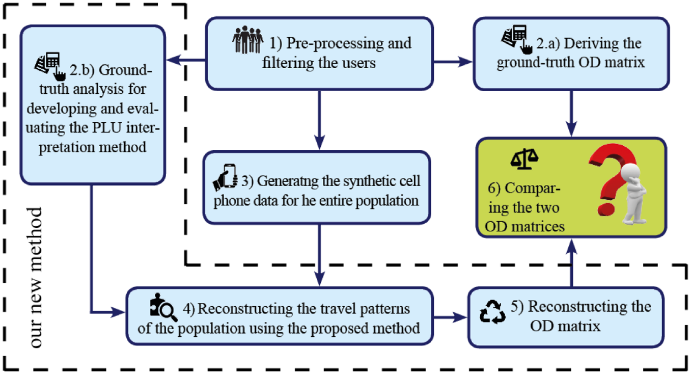
Overall experimental framework.

Kernel-Based Approach of Estimating the OD Matrix

In this section, the features of the proposed KA method are discussed, which mainly focus on the steps 2.b, 4, and 5 of Figure 2. Then, the fundamental concepts of the Bayesian approach are discussed. The next part explains kernel density estimation (KDE), which we used for extracting temporal routines from the training set. The following part explains the applied spatial aggregation on the synthetic GSM data. The comparison measures used in step 6 are also introduced in the last part.

As mentioned previously, PLU periodically observes each cell phone at certain places. However, figuring out whether the person engages in an activity or simply passes by needs further investigations. To identify location type (stay or pass-by) and activity category (home, work, or other), we use a Bayesian classifier. Bayesian inference is regularly applied to estimate distribution parameters from data. In our research, a random 1% sub-sample from the ground-truth data is selected to train the Bayesian classifier. Furthermore, using Bayesian inference, it is possible to update conclusions based on this training set by incorporating new observations ( 20 ).

As indicated before, several studies in the literature have addressed the problem of location type identification in GSM data. Additionally, they have mostly used a time boundary to discern stay from pass-by (e.g., Iqbal et al. [ 13 ], Alexander et al. [ 14 ], and Demissie et al. [ 15 ]); that is, they impose a specific duration as a clear-cut distinction between stay and pass-by. However, in this research, the Bayesian classifier only learned from a training sub-set, randomly selected from the entire travel-activity patterns. In fact, the classifier infers the time boundary from the training set’s temporal routines and applies it to the PLU to distinguish each user’s stationary locations. Temporal routines allude to the distribution of duration and start time of records that are intended to be classified. The major merit of Bayesian inference is that the data in the training set are allowed to “speak for themselves” in determining location type; much more than in the case when the location type would be detected using pre-specified duration boundaries.

The primary logic behind selecting the duration and starting time of events as explanatory variables is that people’s location and activity types are correlated with their temporal patterns.

For instance, trips in urban areas often have duration of less than an hour, whereas stays (i.e., activities) usually last for a couple of hours. Additionally, activity category of home mainly starts in the afternoons or early evenings and takes more than six hours. Work also largely takes more than 5 h; however, they normally start from the morning. Systematically considering these differences in the distributions enabled us to distinguish each event or activity from others.

To understand how we measure the observed duration and start time, consider the example in Figure 1. The first record of each event (i.e., stay or pass-by) is labeled as the start. Accordingly, the start of A, B, C, D, and E are 15:35, 16:20, 16:35, 16:50, and 17:50, respectively. The first record of the next event is labeled as the end of each event, thereby the end times A, B, C, and D are 16:20, 16:35, 16:50, and 17:35, respectively. Since the duration is the difference between the end and start time, with a constant PI (here is 15 min), the durations would be multiples of PI.

Bayesian Classifier

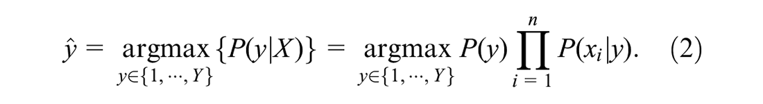
The proposed method, considering pre-specified temporal patterns, estimates the probability of stay and pass-by or activity categories. This approach is general in that it can be applied to diverse mobility patterns and data sources. We leverage the correlation between people's location and activity types with the duration and start times of events, as the event classes influence their temporal patterns. Given the cause (event class), the duration and starting time are conditionally independent (see Russell and Norvig [ 21 ]). Therefore, the full joint distribution can be written as

P (Y, X_{1}, \dots, X_{n}) = P (Y) \underset{i}{Π} P (X_{i} | Y),

(1)

where Y is the event class and can be either location type, with two classes—stay and pass-by—or activity type, with three classes—home, work, and other. Furthermore, $X_{i}$ is the effect and consist of two temporal variables: duration and starting time. Such a probability distribution is called a naive Bayes model—“naive” because it does not account for cases where the effect variables are not truly conditionally independent given the event class. Practically, the naive Bayes method can work surprisingly well, even when the conditional independence assumption is violated ( 21 ).

The naive Bayes model is sometimes called a Bayesian classifier since often maximum a posteriori (MAP) estimation concept is used for classification ( 22 ); that is, the Bayesian classifier assigns the most probable class $\hat{y}$ to the observed data $X$ . Defining $P (y | X)$ as the probability of class $y$ given that $X = x_{1}, \dots, x_{n}$ was observed, the Bayesian classifier evaluates the following maximization scheme (see Yair and Gersho [ 23 ]):

\hat{y} = \underset{y \in {1, \dots, Y}}{argmax} {P (y | X)} = \underset{y \in {1, \dots, Y}}{argmax} P (y) Π_{i = 1}^{n} P (x_{i} | y) .

(2)

The quantities $P (y | x)$ are known as the a posteriori (or class) probabilities, and the Bayesian classifier supplies the MAP decision.

Kernel Density Estimation

The assessment of the a posteriori probabilities using Bayes rule requires an a priori knowledge about the probability density functions of the priors. The probability density function of the priors, which are duration and start time of events (activities and trips), needs to be estimated. Assuming that the observed data points in the training set are a sample from an unknown probability density function, density estimation is the construction of an estimate of the density function from the training set. In this regard, KDE is currently the most popular non-parametric approach for probability density estimation ( 24 , 25 ). Non-parametric density estimation is an alternative to the parametric approach in which a model with a small number of parameters is specified and, using maximum likelihood, the model is calibrated. However, non-parametric density estimator is aimed to estimate the density of a variable from a sample set without assuming any specific form for the density function ( 24 – 27 ). As we generally happen to know very little about the given data, a general smoothness assumption is a reasonable choice. Accordingly, we selected the Gaussian kernel estimation (see Smola et al. [ 28 ]). Therefore, our proposed method is named the kernel-based approach (KA).

Given $N$ independent observations $χ_{N} = X_{1}, \dots, X_{N}$ from an unknown continuous probability density function $f$ on $X$ , the Gaussian kernel density estimator is defined as

{\hat{f}}_{h} (x) = \frac{1}{N} \sum_{i = 1}^{N} ϕ (x, X_{i}; h) \forall x \in IR,

(3)

where

ϕ (x, X_{i}; h) = \frac{1}{\sqrt{2 π h}} \overset{\frac{- {(x - X_{i})}^{2}}{2 h}}{\exp}

(3)

is a Gaussian kernel with location X_i bandwidth $\sqrt{h}$ . Many researchers have focused on the optimal choice of $h$ , since bandwidth selection greatly affects the estimate obtained from the KDE (much more than the shape of the kernel) (e.g., Jones et al. [ 29 ], Sheather and Jones [ 30 ], and Botev et al. [ 31 ]). In this research, bandwidth selection was made by a “rule of thumb” following Scott’s Rule (see Scott [ 32 ]), which suggests that the optimal bandwidth is $n^{\frac{- 1}{d + 4}}$ in which $n$ is the number of data points and $d$ is the number of dimensions.

Spatial Aggregation of GSM Data

As already mentioned, the reported locations in the empirical GSM data generally belong to the antenna that receives the cell phone signal. This naturally means that the highest spatial resolution of the data is the antennas’ coverage areas. Therefore, to demonstrate such a spatial aggregation effect, we used the associated OD zones instead of the exact location coordinates. This means that each OD zone represents one antenna. Also when users only travel inside a zone, their movements are not observed because it is like the person has stayed in one location representing that OD zone (as shown in Figure 3). Under this setting, the hypothetical antennas for each zone are shown in the figure.

Figure 3.

Origin–destination (OD) zones assumed to represent the antennas’ coverage areas.

In addition to the duration and start time, the location of each activity provides information about the activity category. A hierarchical model is applied to the locations (i.e., OD zones) in the training set to estimate the a priori for each spatial zone in the Bayesian model. This hierarchical model estimates the probability of each activity category in each OD zone. The activity category is drawn from a categorical distribution with the parameter specific to each zone. This parameter is drawn from a Dirichlet distribution with parameter $α$ assumed to be unique among all the zones (we assumed it be a vector of one which is equivalent to a uniform distribution).

θ_{d = 1 \dots M} ~ Dirichle t_{K} (α)

(4)

z_{d = 1 \dots M, n = 1 \dots N_{d}} ~ Categorica l_{K} (θ_{d})

(5)

where

z the activity category of the observation,

$α$ the hyper-parameter vector of the Dirichlet prior,

M the number of zones,

N the number of records, and

K the number of assumed activity categories (three here).

We investigate whether considering the spatial variable under the mentioned setting will improve the model accuracy for our data set.

OD Matrix Comparison

To evaluate the performance of the proposed method for OD matrix estimation, as well as evaluate the effect of polling frequency hereon, a metric is needed that measures the accuracy of the estimated OD matrix against the ground-truth OD matrix. OD matrices can be compared in two complementary ways. Firstly, the degree to which the estimated OD matrix correctly represents the absolute amount of demand between all individual OD pairs. Secondly, the degree to which the estimated OD matrix correctly represents the relative demand pattern seen across OD pairs ( 33 ).

For the former absolute comparison, traditional measures such as mean absolute error (MAE) (see Ashok and Ben-Akiva [ 34 ] and Lo and Chan [ 35 ]), and R-squared (see Tavassoli et al. [ 36 ]) can be used. Here we use MAE to compare the OD pair values in the two matrices.

For the latter relative comparison, the geographical window-based structural similarity index (GSSI) ( 37 ) is capable of distinguishing structural differences owing to the geographical closeness of OD zones. Here we use GSSI to compare the correlation of OD pair values across geographical windows (where OD zones with geographical proximity belong to the same window).

Method Implementation

The experiments are done on daily activity plans of agents derived from the nationwide activity-based model ALBATROSS ( 38 ). All agents are selected for which at least one household member uses the mode car to perform at least one activity within the Amsterdam region ( 39 ). This leads to the activity plans of 22,000 agents during a representative working day.

Note that we use synthetic (model-generated) activity plans in the KA step, our method estimates temporal patterns of location and activity types. Therefore, to ensure generalizability of our method toward empirical travel diary data, it is important to emphasize that the ALBATROSS model does not assume any a priori (theoretical) distribution of activities, but instead uses decision trees that are directly calibrated from travel diaries. ALBATROSS implements a sequential decision-making process to generate an individual’s schedule. Empirical demand data are employed to induce a decision tree for each step in the scheduling process ( 40 ). Thus, the model framework (i.e., decision tree) does not restrict the activity’s temporal pattern to a specific distribution. Decision trees can describe discontinuous impacts of discrete attribute variables on decision making. Therefore, our KA step's ability to capture the temporal distribution of location and activity types is grounded in the underlying empirical travel diaries. This is important, because otherwise if the synthetic data were based on a model that adopts a (parameterized) distribution function to simulate activity patterns, then the temporal distributions might have been artificially imposed by the model structure (i.e., a model assumption, not a model result).

The agents’ activity plans are simulated using MATSim ( 41 ), which is an open-source agent-based transport simulation model. The MATSim model output is used to generate synthetic PLU data as follows.

The experienced plan output contains basically the traces of each agent in our data set. This file represents the ground-truth OD matrix. One percent of these agent traces is sampled to be used as travel diaries in the KA step of our method (to estimate the Bayes model distinguishing stay and pass-by locations, and detecting the activity category).

The snapshot output contains the records of all agents per snapshot interval, which is conveniently used (with slight modifications concerning formatting) to generate our synthetic PLU traces. The resulting PLU format is shown in Figure 1a in which the associated OD zone represents the location.

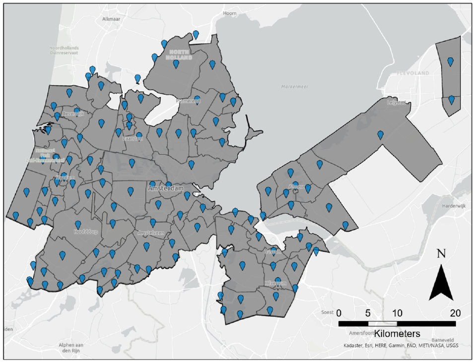
The OD zoning system is an aggregated version of 4-digit postal codes in Amsterdam leading to 115 zones (Figure 4a). When computing the GSSI metric (i.e., structural similarity between OD matrices) these are aggregated to 50 geographical windows as displayed in Figure 4b.

Figure 4.

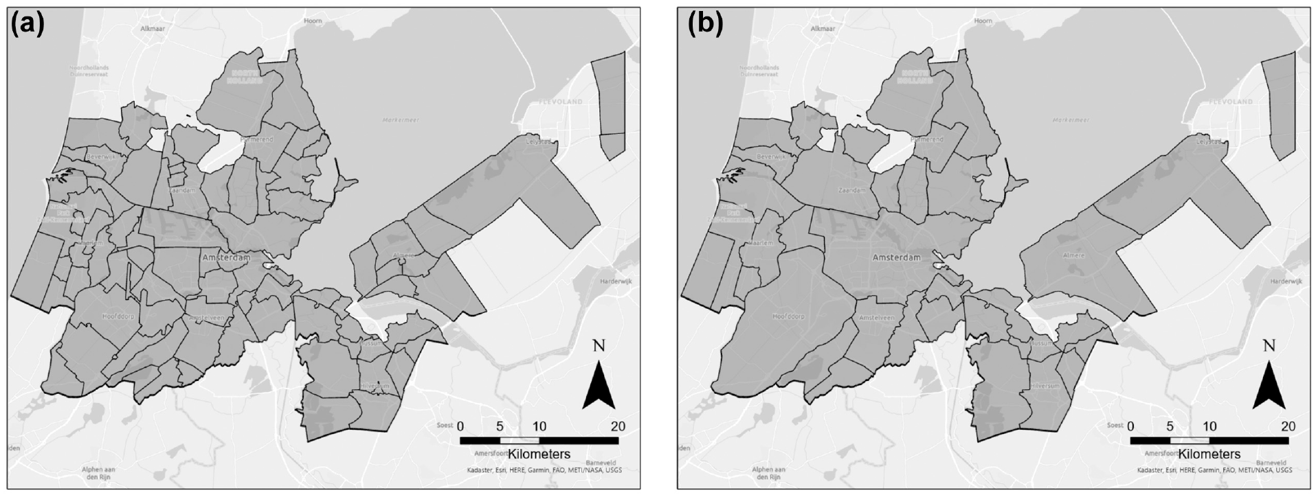
Zone boundaries applied to this study: (a) Amsterdam origin–destination (OD) zones and (b) high-level boundaries as geographical windows.

Results and Discussion

In the following, we present the KDE results and evaluate the KA performance in detecting location types and in detecting activity types. This is done for a random training set. Then we show how robust these results are against selecting the training set. Finally, we shows the accuracy of the reconstructed OD matrices for a range of PIs.

KDE Results

As mentioned in the previous part, the proposed methodology is trained using a 1% subsample of the ground-truth data, and its performance is tested on the entire ground-truth data set.

An example result of applying KDE on the training set (based on one example random seed for selecting the training set) is given Figures 5 and 6 for location and activity category detection, respectively. For each location/activity type, two distributions of duration and starting time are calculated. Having assumed two location types of stay and pass-by and three activity categories of home, work, and other, ten distributions are fitted to the training data. The KDE simply fits a smooth curve to the data and introduces the likelihood required for the Bayesian classifier. As we usually happen to know very little (in our case 1% of the population) about the ground-truth, a smoothness assumption for the training set’s density estimation is justifiable. The smoothness assumption prevents over-fitting caused by sparse sampling when the training data, like in our framework, come from a small proportion of the population. It is worth mentioning that the smoothing assumption can be relaxed in case the training data represent the entire population more thoroughly.

Figure 5.

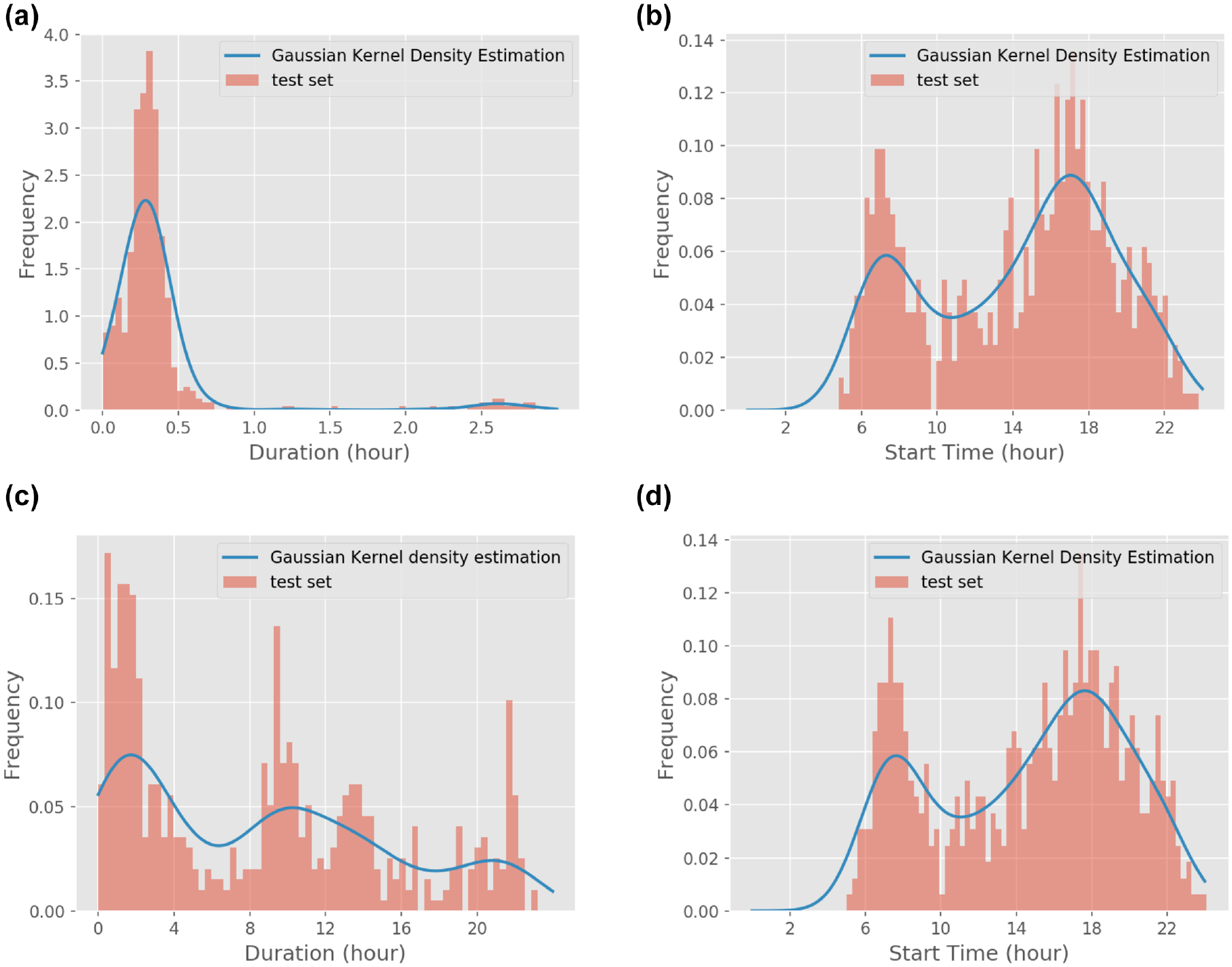
Application of kernel density estimation (KDE) for location type detection: (a) trip duration, (b) trip start time, (c) activity duration, and (d) activity start time.

Figure 6.

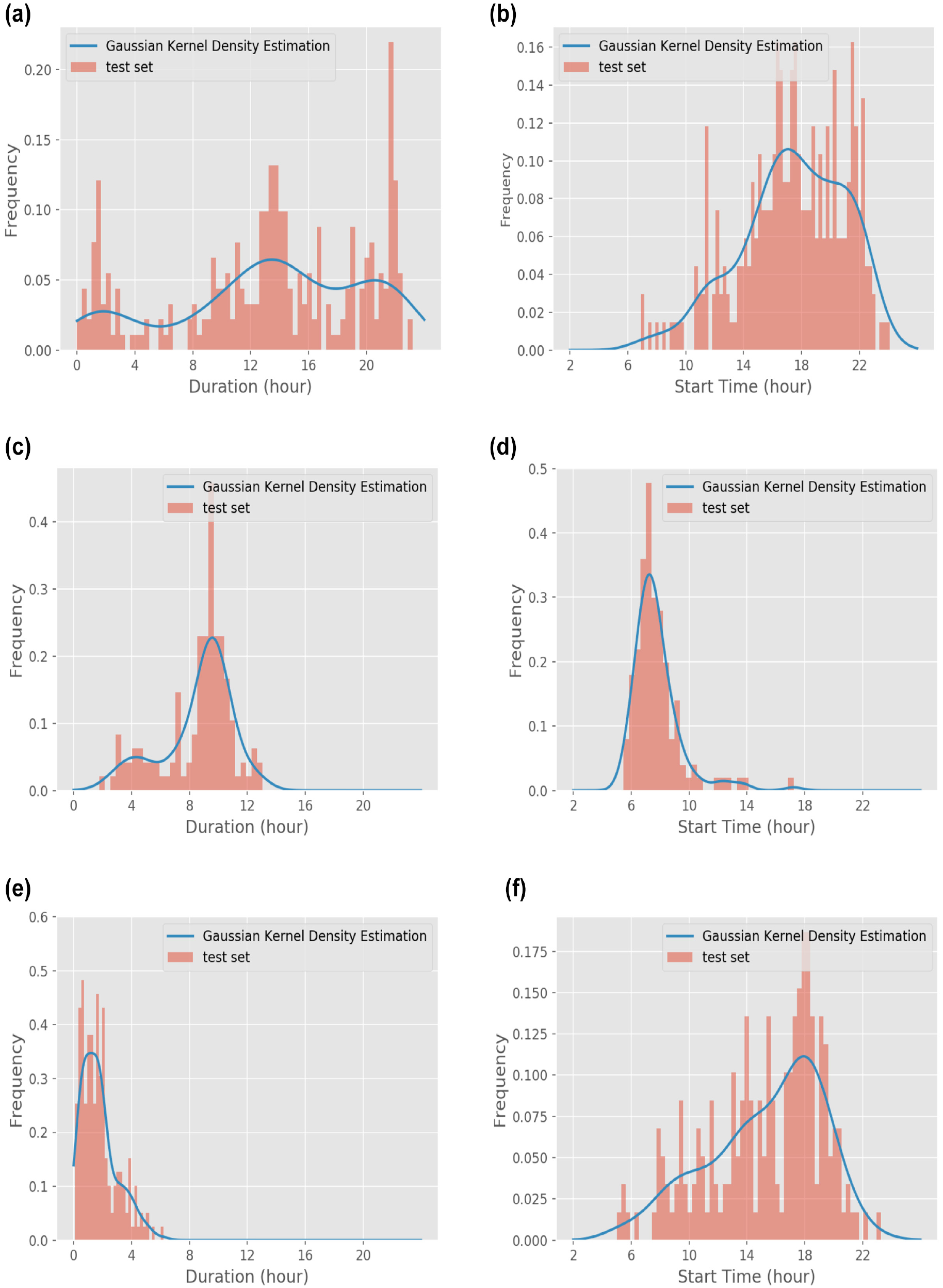
Application of kernel density estimation (KDE) for activity type detection: (a) home duration, (b) home start time, (c) work duration, (d) work start time, (e) other duration, and (f) other start time.

It can be inferred from Figure 5, b and d , that the start time pattern of trips and activities follow a close distribution. Consequently, the KA distinguishes the event types merely based on the duration distributions which follow different pattern in each event type. As a result when duration patterns of activity and trip are similar, misprediction of location type takes place. Considering Figure 5, a and c , mispredictions might happen when duration is less than 45 min.

For such cases, the location of the record plus temporal features might give a more precise prediction of the event and activity category. However, this is only true if the spatial resolution of the data is high enough to recognize different land-use types from each other. In fact, in dense urban environments like Amsterdam, assuming high spatial resolution for GSM data is not realistic. Because various events and activity categories take place in a small area and to estimate a reliable probability of each, the GSM antennas have to be unnecessarily closer to each other. Perhaps for sparsely developed urban environments, using spatial variables in the KA model becomes reasonable.

KA Performance Concerning Location Type

The performance of the KA classifier for location type detection is shown by the confusion matrix in Table 1. The results show that 92% of all stay and 97% of all pass-by locations were detected correctly, using the proposed methodology (overall, in 94.4% of the time, the location type was distinguished correctly). Based on Table 1, KA underestimated the stay locations. Accordingly, overestimation in pass-by locations occur at the same time. Therefore, in stay detection, we often had false-negative errors, and in pass-by detection, false-positive errors happened the most.

Table 1.

Confusion Matrix of Applying the Methodology on the Entire Ground-Truth for Location Type Recognition

	Observed stay	Observed pass-by	Total predicted
Predicted stay	54,231 (91.8%)	1,799 (3%)	56,030 (47.4%)
Predicted pass-by	4,822 (8.2%)	57,254 (97%)	62,076 (52.6%)
Total observed	59,053 (100%)	59,053 (100%)	118,106 (100%)

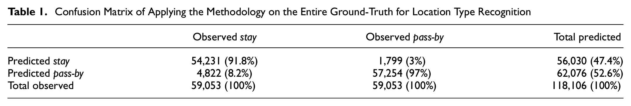
As already mentioned, owing to closeness of stay and pass-by starts, duration of events has a more significant role in differentiating them. Observing the results showed that the minimum duration of correctly recognized stays was about 44 min. Therefore, it seems that KA specifies a duration threshold to separate stays from pass-bys. Although this threshold is selected by analyzing the temporal distributions in the training set, it cannot entirely divide stays and pass-bys owing to overlaps around the threshold. In fact, our analysis shows that about 88% of activities have duration of more than 44 min, whereas, 96% of trips endure less than 44 min. Thus, activities are less probable to be recognized. This justifies the underestimation in activity detection in Table 1.

Variable Selection and Model Performance in Activity Category Inference

In our model we included predictors that help maximize the activity category accuracy. To select the model’s explanatory variables, we considered three states: First, only spatial variable; second, spatial and temporal variables together; third, only temporal variables. The associated confusion matrices are shown in Tables 3, 4, and 5. The overall performance of the classifier for activity category detection for each of these states is shown in Table 2. The precision score is a ratio that shows the quality of positive predictions made by the model and is defined by the number of true positives divided by the total number of positive predictions so that 100% precision implies no false positives. However, this typically coincides with a lower recall score, which is defined as the number of true positives divided by the sum of true positives and false negatives, so that 100% recall implies no false negatives. In an imbalanced classification, the balanced accuracy is the average of the recall score obtained in each class.

Table 2.

Performance Metrics of the Three States used for Activity Type Recognition

State	Only spatial variable	Both spatial and temporal variables	Only temporal variables
Precision score	0.4211	0.9019	0.9058
Recall score	0.4792	0.8931	0.8969
Balanced accuracy	0.3659	0.9086	0.9144

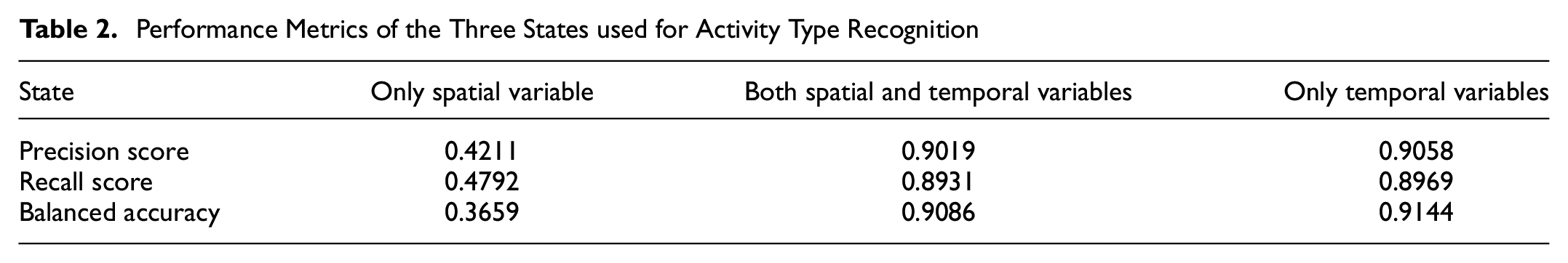
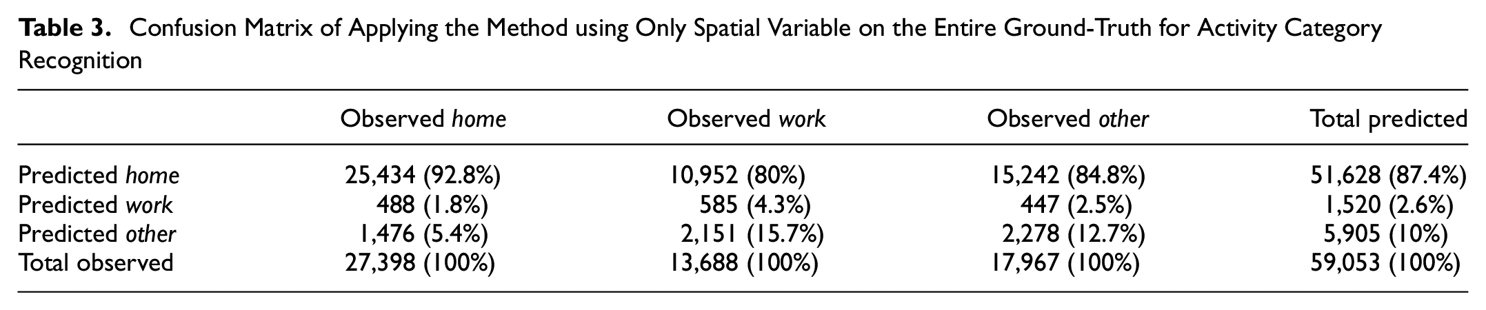
The results (Table 2) show that considering only OD zones leads to accuracy scores as low as 36.6%. Also, based on Table 3, this model seems to be biased toward detecting home as more than 80% of other categories are incorrectly labeled as home. Figure 7 also shows that in most OD zones the probability of home is more than the other two.

Table 3.

Confusion Matrix of Applying the Method using Only Spatial Variable on the Entire Ground-Truth for Activity Category Recognition

	Observed home	Observed work	Observed other	Total predicted
Predicted home	25,434 (92.8%)	10,952 (80%)	15,242 (84.8%)	51,628 (87.4%)
Predicted work	488 (1.8%)	585 (4.3%)	447 (2.5%)	1,520 (2.6%)
Predicted other	1,476 (5.4%)	2,151 (15.7%)	2,278 (12.7%)	5,905 (10%)
Total observed	27,398 (100%)	13,688 (100%)	17,967 (100%)	59,053 (100%)

Figure 7.

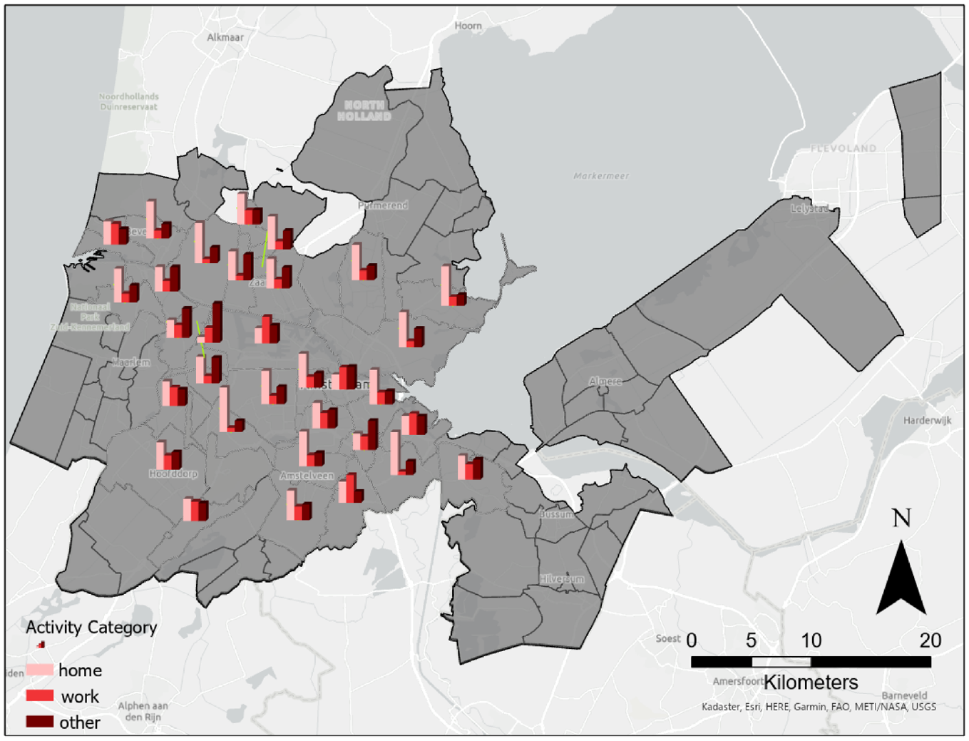
Average probability of each activity category based only on location origin–destination (OD) zone.

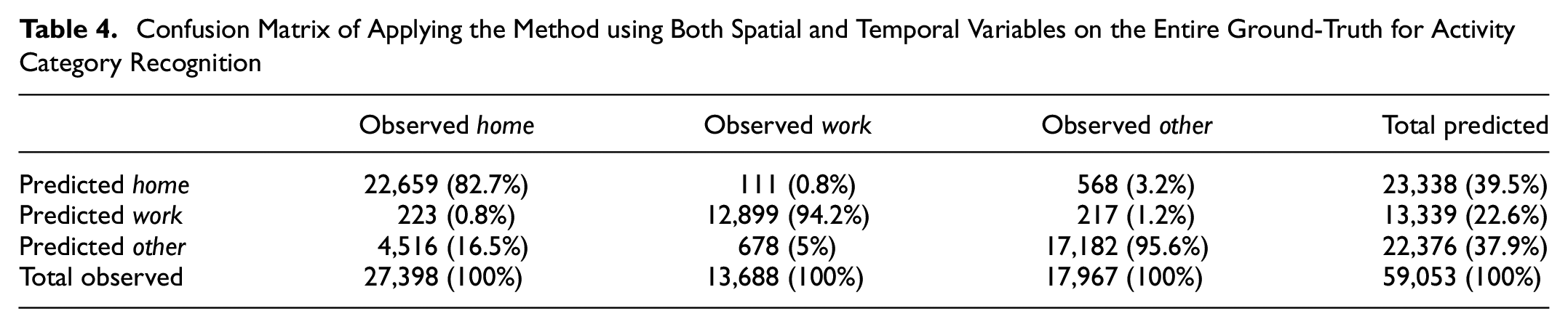
Adding temporal variables in Table 2 increases the overall accuracy to around 90%. However, owing to the presence of the spatial variable, the results are slightly biased toward home (Table 4). Table 5 confirms this because as the accuracy of home detection is reduced, the accuracy of work and other increase. Overall, the highest accuracy is achieved by considering only temporal variables in Table 2. Therefore, using location does not improve the overall activity category detection under the considered spatial level of aggregation, and using only temporal variables suffices. If detecting home is of a higher priority, considering location alongside temporal variables becomes a preference.

Table 4.

Confusion Matrix of Applying the Method using Both Spatial and Temporal Variables on the Entire Ground-Truth for Activity Category Recognition

	Observed home	Observed work	Observed other	Total predicted
Predicted home	22,659 (82.7%)	111 (0.8%)	568 (3.2%)	23,338 (39.5%)
Predicted work	223 (0.8%)	12,899 (94.2%)	217 (1.2%)	13,339 (22.6%)
Predicted other	4,516 (16.5%)	678 (5%)	17,182 (95.6%)	22,376 (37.9%)
Total observed	27,398 (100%)	13,688 (100%)	17,967 (100%)	59,053 (100%)

Table 5.

Confusion Matrix of Applying the Method using Only Temporal Variables on the Entire Ground-Truth for Activity Category Recognition

	Observed home	Observed work	Observed other	Total predicted
Predicted home	22,458 (82%)	52 (0.4%)	175 (1%)	22,685 (38.4%)
Predicted work	289 (1.1%)	12,963 (94.7%)	248 (1.4%)	13,500 (22.9%)
Predicted other	4,651 (17%)	673 (4.9%)	17,544 (97.6%)	22,868 (38.7%)
Total observed	27,398 (100%)	13,688 (100%)	17,967 (100%)	59,053 (100%)

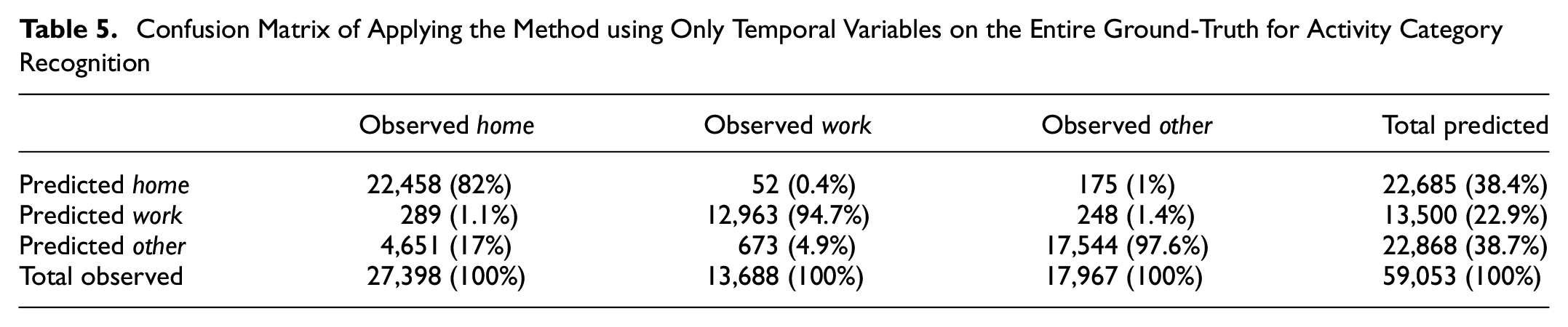
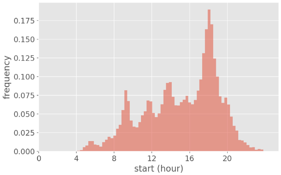
The results in Tables 5 and 4 also roughly show that false-negative errors occur mostly for home category. Moreover, most of the false-positives are revealed for other. Focusing on when the method fails to detect the right activity type, Figure 8 presents the distribution of false-negative error in predictions over duration for home. Since the long duration of home discriminate this type of activity from other categories, false negatives mostly occur when it comes to shorter duration (less than 5 h). Figure 9 shows the actual duration distribution of other.

Figure 8.

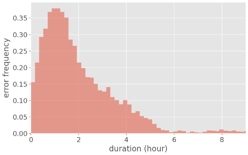
False negatives based on the duration of home.

Figure 9.

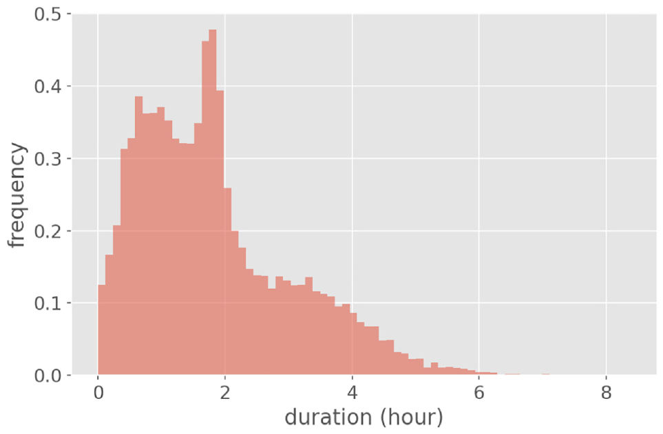
Actual duration distribution of other activities.

Similarity of the distributions in Figure 8 and 9 shed light on why the methodology might confuse home with other. Moreover, Figure 10 presents the distribution of false negative error in predictions over start time for home. Figure 11 displays the actual start time distribution of other.

Figure 10.

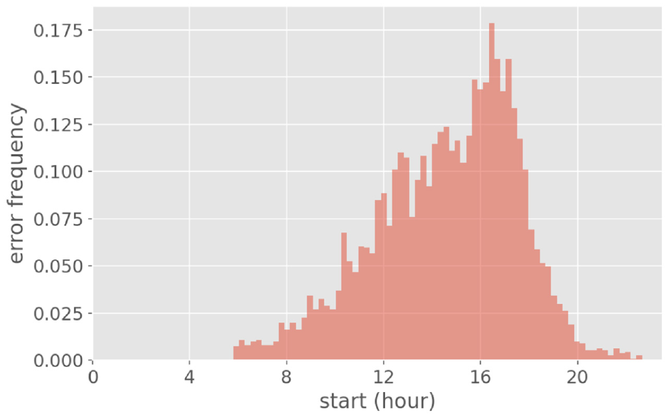
False negatives based on the start time of home.

Figure 11.

Actual start time distribution of other.

The afternoon peak in both figures give rise to confusion of home with other activities. Thus, activity type is estimated based on the start time and duration of stay, but under specific conditions such as short activity duration in the early evening the temporal distributions are nonconclusive; that is, owing to the sporadic closeness of the temporal pattern of home and other, misprediction may occur.

Sensitivity of KA Results to Training Set Sampling

To evaluate the sensitivity of the randomly sampled training set (seed and size), the analyses in the previous sections were repeated using 50 different seeds. Figure 12 presents the KA performance (i.e., accuracy) in location-activity type detection across these 50 seeds.

Figure 12.

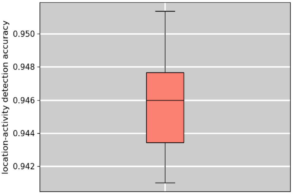
Kernel-based approach (KA) performance in location-activity detection on 50 different random seeds for selecting the training set.

The KA performance appears robust for different random seeds. This is further tested statistically using a Chi-square test on two random sub-samples each containing the performance for 25 different seeds (i.e., training sets). With a significance level of 0.05, the null-hypothesis that the two sub-samples belong to the same distribution could not be rejected (i.e., we cannot conclude that the KA performance derived from different sub-samples of random training sets would yield different distributions).

In the previous sections we evaluated the KA performance for a single random training set. The results of the Chi-square test indicate that a sample size of 25 is robust to evaluate the KA performance. Therefore in the following section the accuracy of the reconstructed OD matrix is evaluated based on 25 experiment runs (i.e., across 25 different random seeds for training set sampling).

OD Matrices Comparison Results

This part presents the results of applying KA on the generated PLU from the ground-truth using MATSim. We considered 18 various PIs in generating the PLU, which are 30 and 60 s, every 5 min from 5 to 60 min, and every 15 min from 1 to 2 h. Since non-linearity and variation of results are high for PIs less than 2 h, these intervals were selected Moreover, for more clarification on the correlation of randomness of the results and the underlying PI, all results were calculated for 25 different random seeds (for selecting the training data from the ground-truth). Having derived the OD matrices for the morning peak (6:30 to 9:30) for both PLU and the ground-truth, we compared the actual and reconstructed outcomes using two performance indicators:

MAE between OD pairs of reconstructed and ground-truth OD matrices, which compares the OD pairs values, and

GSSI (for further information refer to Behara et al. [ 37 ]), which captures the structural similarity between the two matrices.

Figure 13 describes the MAEs resulted from comparing the ground-truth OD cells (as the observed values) and the reconstructed OD cells (as the predicted values) over a range of PIs. It is reasonable to see that the average value of MAE gradually increases by reducing the PF.

Figure 13.

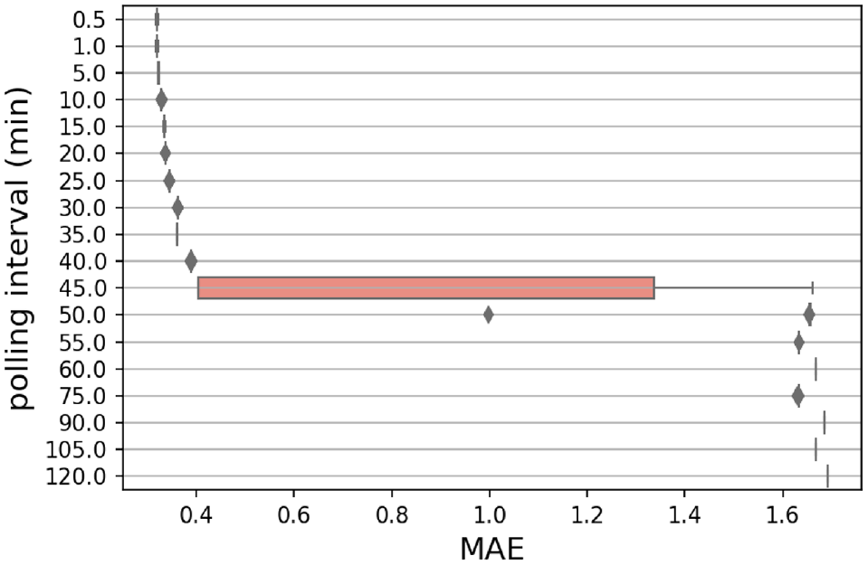
Mean absolute errors (MAEs) related to origindestination (OD) matrices resulted from 25 different random seeds over 18 different polling intervals (PIs).

Conversely, drops and jumps in the MAE values (from 45 to 120 min) might be attributable to the particular timing pattern of travels and activities (i.e., the context of the data result in such changes). In fact, it seems that the reliability of the method drops after PI = 45 min.

To clarify the reliability fall, Figure 14 shows an example of a user’s traces. Assuming that the letters show the OD zone, the user’s actual traces, in Figure 14a, are {A, B, C, B}, in chronological order. However, the traces interpreted from the PLU with PI of 1 min (Figure 14b) are {A, B, B} which lacks the detection of C. This occurs owing to duration of staying in C (30 min), which was less than the duration threshold (about 45 min); thus, the record was interpreted as pass-by. Likewise, when PI = 40 min (Figure 14c), the traces are {A, B, B}, but owing to another reason—we lost activity C owing to stay duration less than the PI value. Since travel demand derives from people’s needs and desires to participate in activities, there could be a condition to compensate for such errors: When the interpreted travel pattern include similar (close in location coordinates) successive activities, a missed activity is assumed to be in between. It is located in the farthest record location between the two similar activities. The start time and duration could be derived using speed data and the distances between the locations.

Figure 14.

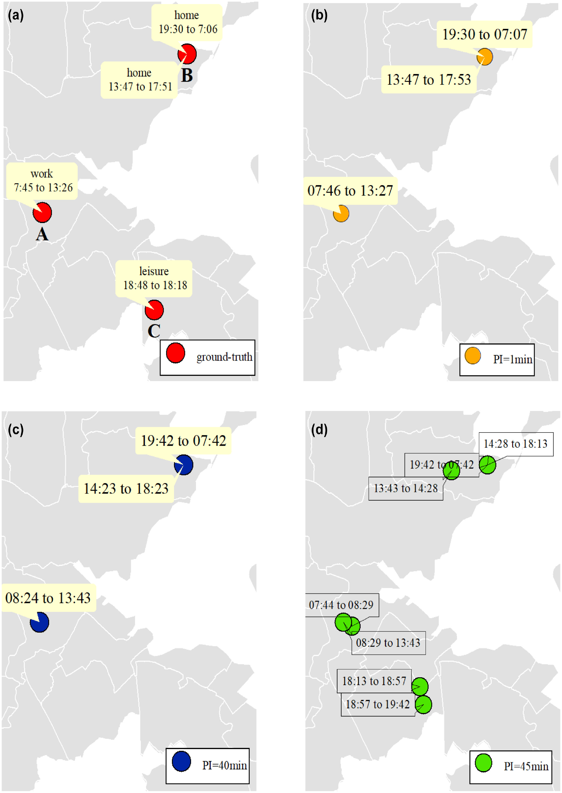
Example traces of a user: (a) ground-truth traces, (b) interpreted traces when polling interval PI = 1 min, (c) interpreted traces when PI = 40 min, and (d) interpreted traces when PI = 45 min.

Important deviations are seen in Figure 14d. Since PI = 45 min exceeded the duration threshold (44 min), any record was considered as stay and the method’s job was limited to only cluster the similar records. Therefore, a significant number of imaginary stays (i.e., activities) were generated; therefore, the traces in Figure 14d were {A, A, B, B, C, C, B} and instead of having four activities, we detected seven. The major issue here is that the travel time between all these activities is zero, which is not feasible. Moreover, detecting and alleviating these massive errors is complicated owing to lack of information. Consequently, it is recommended to exclude users or scenarios with PI values exceeding the duration threshold, as this boundary represents a critical value, after which a sudden change in the performance of the KA for OD estimation happens. Approximately 10 minutes after reaching this critical value, the variance appears to decrease to levels even lower than before, indicating greater stability of the results against different random seeds underlying the training set. This phenomenon happens because in PIs more than 50 min, the KA cannot detect short-time activities anymore. In other words, the remaining activities are of long durations. For instance, home is more robust against random seeds since its duration is much higher than the PIs discussed here.

As another performance measure indicator, comparing the structure of OD matrices, we derived the GSSI for each of the PIs with 25 random seeds (Figure 15). Basically, GSSI is in the range of [0,1] and the higher GSSI indicate higher structural similarity of matrices. Therefore, the gradually descending trend is perceivable (owing to the inability to detect short time activities with durations less than PIs) before the duration threshold, but high variation is also noticeable. Concerning this, a higher PI increases the probability of missing the activity, even when the PI is still below the activity duration. In fact, higher PIs increase the delay range of detecting the start and end of activities. As the range of interpreted duration increases, the variation also rises, making misidentification more likely to occur. Apart from the indicated rationale, errors owing to the data characteristics might also produce variation in the results.

Figure 15.

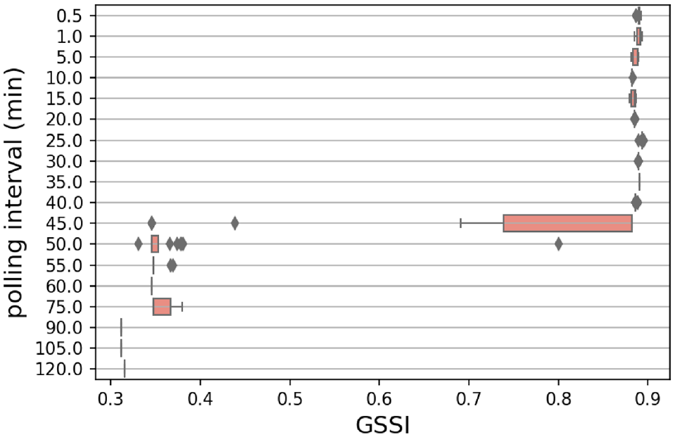
Geographical window-based structural similarity index (GSSI) related to (OD) origin–destination matrices resulted from 25 different random seeds over 18 different polling intervals (PIs).

To understand the changes in Figure 15, note that the interpreted duration is a multiple of PI values. Furthermore, as mentioned previously, about 88% of activities have duration of more than 44 min (the duration threshold), whereas, 96% of trips endure less than 44 min. Thus, activities are more probable to be misidentified (i.e., stays have more false negatives than pass-bys). However, under a special condition, activities’ false negatives decrease.

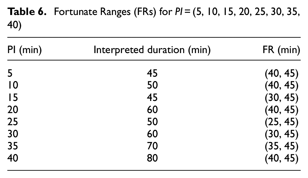
To take a closer look at the results in Figure 15, Figure 16 shows the GSSI only for PIs less than the duration threshold. Since the input of KA is the interpreted duration, identification of a stay requires to have an interpreted duration more than the duration threshold (45 min), even if the actual duration is less than the threshold. For instance, when PI = 10 min and interpreted duration = 50 min, it is probable that the record be considered as stay even if its duration be in the range of (40, 45) min. We call this range the fortunate range (FR), which we define only to explain the results in Figure 16. The length of FR causes the changes in GSSI value for PIs less than the threshold. The FRs for our other PIs are shown in Table 6. Notice that once the interpreted duration reaches the duration threshold, it is considered as stay. The longest FR belong to PI = 25 min. The same PI got the highest GSSI in Figure 16.

Figure 16.

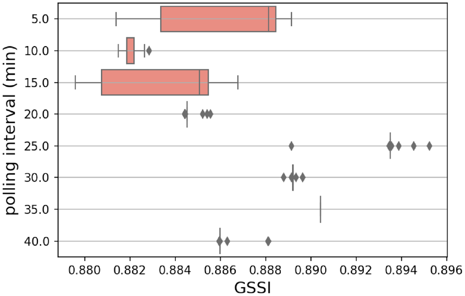
Geographical window-based structural similarity index (GSSI) related to origin–destination (OD) matrices resulted from 25 different random seeds over eight different polling intervals (PIs).

Table 6.

Fortunate Ranges (FRs) for PI = (5, 10, 15, 20, 25, 30, 35, 40)

PI (min)	Interpreted duration (min)	FR (min)
5	45	(40, 45)
10	50	(40, 45)
15	45	(30, 45)
20	60	(40, 45)
25	50	(25, 45)
30	60	(30, 45)
35	70	(35, 45)
40	80	(40, 45)

Conversely, when the interpreted duration falls near the duration threshold, the variation spikes. Accordingly, PI = 5,15 min have high variances. In fact, this variation is higher for PI = 15 min owing to longer FR—more stochasticity. Naturally, between four PIs of 5, 10, 20, and 40 min that have the similar FRs, the lower PI gets the higher GSSI. PI values of more than the duration threshold are not discussed owing to poor performance of KA and many unreal generated activities.

Overall, it seems that when false negatives of stays are more than that of pass-bys, the longest FR with a minimum PI results in the highest GSSI; the most structurally similar reconstructed OD matrix to the ground-truth matrix. In our case, with duration threshold of about 45 min, PI = 25 min yields the highest GSSI. Basically, under the mentioned circumstances, with duration threshold of T, the ideal PI is $T / 2 + ϵ$ where $ϵ$ is a very small value.

Research Limitations

This research had several strengths: It certainly adds to our understanding of the effects of temporal characteristics of PLU data on the accuracy and robustness of the resulting OD matrix. It also proposes a data-driven method for interpreting the raw PLU data. Nonetheless, these findings must be interpreted with caution, and several limitations should be borne in mind as follows:

Limited synthetic data: Real-world mobile phone datasets can offer ample information about millions of mobile phone users. Nevertheless, their limitation concerns the privacy issue and the difficulty of carrying out reliability and validation experiments (owing to the unavailability of the ground-truth). To conduct operational tests and evaluations, we used synthetic (travel diary and GSM) data, thus including the ground-truth by design and without any privacy concerns. However, the question is whether our findings are generalizable toward empirical data. It is worth mentioning that the ALBATROSS model (based on which our data are generated) does not assume any a priori (theoretical) distribution of activities but instead uses decision trees that are directly calibrated from travel diaries. Therefore, the model structure has not artificially imposed temporal distributions. However, a sampling bias in the original travel diary used to train ALBATROSS might be affecting the data’s representativeness in describing the entire population.

Conversely, the Bayesian model is naturally resistant to non-informative predictors. Nevertheless, owing to the naive nature of our model, incorporating the location in addition to temporal variables in activity category detection slightly reduced the overall accuracy. This is because, in naive Bayesian models, different prior variables are assumed to be conditionally independent. This assumption can be avoided by establishing the correlation of prior variables, which usually require a more extensive data set than the data available in this study. Therefore, we acknowledge a need for a future study (e.g., a longitudinal study) to consider a fully Bayesian model to comprehensively describe the relationship between the explanatory variables.

Mismatch between traffic analysis zones (TAZ) and base station coverage zones: This research assumes that the base station coverage area is the same as its associated TAZ. However, there is a mismatch between the antenna’s coverage zone and TAZ in practice. But we ignored this mismatch because the base station coverage area is typically much smaller than a TAZ. In fact, in the urban areas, the size of a typical TAZ is about 2–5 km, and that of a base station zone is about 50–200 m ( 42 ). To investigate further, Figure 17 shows the cumulative density function (CDF) of TAZ sizes. Accordingly, the average TAZ size is about 15 km which naturally contains tens of base stations.

Therefore, the influence of the size of base station areas on the quality of TAZ division is not significant in urbanized areas (as is Amsterdam). In other areas and to generalize the analysis, one needs base station distribution and location data to account for the errors in the traffic activity analysis. It is worth pointing out that the TAZs seem too large to capture short-distance trips. Figure 18 shows the CDF of the trip distances in our study. Accordingly, more than $10 %$ of the trip distances are less than 3 km, despite considering only car mode. Undoubtedly, adding active modes of transport to the analysis makes this proportion much higher. Despite the large extent, coarse-sized TAZs used for transport planning (as used here) will inevitably eliminate such short-distance trips.

Positioning accuracy and disturbance (ping-pong handover): Overall, OD accuracy is affected by multiple factors, namely positioning interval, positioning accuracy, and positioning disturbance (ping-pong handover). This paper only discusses the effects of positioning intervals because we assume this factor can be decoupled from the other two and investigated in separate studies. Future studies can empirically study positioning accuracy in the presence of positioning disturbances.

Disregarding up-scaling the sample OD matrix toward the OD matrix of the entire population: The available GSM data typically pertain to a sample of the population. Therefore, the use of GSM data to estimate OD matrices is a two-part problem (e.g., Iqbal et al. [ 13 ], Toole et al. [ 43 ], and Mohanty and Pozdnukhov [ 44 ]). The first part is to go from GSM traces of the sample population to an OD matrix of that sample (usually using zonal and temporal aggregation). The second step is to go from the OD matrix of the sample to the OD matrix of the entire population (usually using weighted scaling). In this paper, we focus on the first part of the problem—that is, to derive an OD matrix for the (sampled) GSM traces—while addressing how the PI affects the task of zonal and temporal aggregation.

Disregarding the mode of transport: Generally, the Bayesian classifier is sensitive in modeling the activity pattern with a low sampled mode. This study only uses the data belonging to users with the car mode. However, there might be some challenges to the approach’s generalizability for practical implementation which can be a direction for further research in the future. Although it is worth mentioning that, on analyzing a raw set of GSM data, the mode of transport can be distinguished in two ways: (1) by adjusting our model to detect the mode of transport within the framework and (2) by considering the mode detection as a separate problem before our framework. The former way of addressing mode detection will increase the model errors significantly as the kernel density estimator uses the features of all modes, with different spatiotemporal patterns, simultaneously. Different modes of transport have a different distribution of features, especially concerning trip duration. Therefore, the Bayesian classifier adapts itself to put the cutting edge between stay and pass-by on an average value for all modes, producing high deviation relative to associated observed values.

In this regard, Huang et al. ( 45 ) reviews the literature on transport mode detection with mobile phone network data. Accordingly, mode detection should take place after location type detection because the trip properties like speed, duration, start time, and stay location help detect the mode. However, some studies used geographic data to extract main transport modes based on proximity to main roads, shortest paths, or train stations with the public transport timetable. These map-matching methods can still be applied before location-type detection. A suggestion to improve the generalizability of the KA method is to adapt mode detection inside KA using an iterative process. The major steps are as follows: (1) location-type detection for the entire data (containing all the modes), (2) applying a similar method we used for activity-type detection to extract the main modes of transport, and (3) re-detection of location type separately for each detected mode. This iterative process potentially leads to simultaneously detecting location types and modes of transport. Validating the suggested iterative approach requires another research and data available on all modes of transport.

Figure 17.

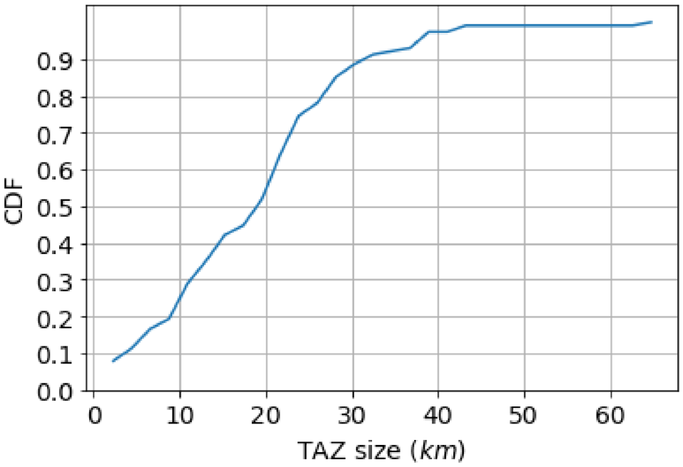
Cumulative density function (CDF) of the traffic analysis zone (TAZ) sizes in our study.

Figure 18.

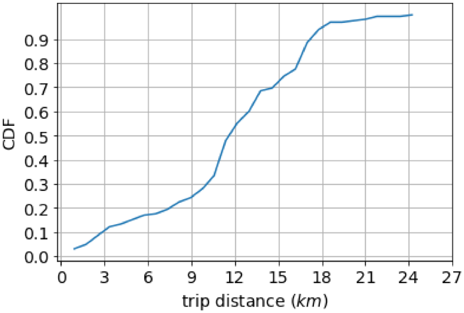
Cumulative density function (CDF) of the trip distances in our study.

Conclusion and Outlook

GSM data allow observing the location of users over time, but the challenge remains in discerning activity (stay) locations. For this, additional information is needed. We show that a KA can provide this location detection when based on travel diaries of a sample of as little as 1%.

The results presented in this paper describe how temporal characteristics (i.e., aggregation and discretization) of GSM data affect the accuracy and robustness of the reconstructed OD matrix. It seems that the PI and temporal criterion (i.e., the duration threshold to distinguish stay from pass-by locations in each user’s traveling traces) jointly affect the OD matrix reconstruction.

As perhaps expected, we show that the accuracy of the reconstructed OD matrix gradually declines with higher PI. However, we also show that the reliability of the KA accuracy declines substantially when PI exceeds the duration threshold. Therefore, the combination of larger PI (in data collection) than duration threshold (in OD matrix reconstruction) is best avoided.

Depending on the data context (observable in the training set), fortunate ranges exist for activities with durations and PI less than the duration threshold. These ranges exist owing to the data temporal discretization and different interpreted and actual durations. In fact, since the interpreted duration of events defines their type, if the interpreted duration of a stay is more than the duration threshold (even if the actual duration of it is less than the duration threshold), it would be recognized as a stay. Our results imply that an “optimal PI” seems to exist which brings about the most structurally similar OD matrix to the ground-truth one. This PI is the minimum value that results in the longest FR. If the duration threshold has the value of T (it can be assumed to be the minimum stay duration resulting from applying KA on the training set) the optimal PI is about $T / 2 + ϵ$ , where $ϵ$ is a small value. Moreover, the $ϵ$ better be selected in a way that the interpreted durations are not close to the duration threshold. This increases the robustness of the results against the random seeds adopted for selecting the training set. For instance, when the duration threshold is 45 min, we assume the PI to be 25 min for which the minimum interpreted duration (more than duration threshold) is 50 min.

Unavoidably, as it is inherent to GSM data, short-duration activities will remain difficult to detect. Importantly, this study has shown how non-detection or misidentification mainly occurs in cases of unusual activity-travel behavior; for example, short-duration home activities during the afternoon peak are susceptible to be confused with other activities owing to similar temporal patterns.

Many models, particularly those which are based on regression slopes and intercepts, will estimate parameters for every term in the model. Therefore, having non-informative variables can add uncertainty to the model performance. However, the Bayesian model is naturally resistant to non-informative predictors. Still, owing to the naive nature of our model, one needs to select the explanatory variables carefully to avoid biased inferences. Depending on the spatial aggregation level, the location of records might help to infer the activity type. Spatial aggregation is associated with the density and distribution of antennas across the network. In our study, the location of the records does not provide much data on the activity categories. Therefore, incorporating the location in addition to temporal variables in activity category detection did not significantly change the accuracy. In fact, it even slightly reduced the overall accuracy. This may appear counter-intuitive, but is because, in naive Bayesian models, different prior variables are assumed to be conditionally independent. This assumption can be avoided by establishing the correlation of prior variables, which usually requires a more extensive data set than the data available in this study.

In addition to temporal characteristics, this method could use speed and distance between the records to decide on their type (stay or pass-by). For instance, initially, we assumed that the travel time is the Euclidean distance between two location coordinates divided by the average speed extracted from the training data. However, this assumption did not improve our estimations (i.e., OD matrix) owing to two reasons: First, the actual speed has a variety of ranges depending on time, space, and user’s behavior (and mode of transport but here we only considered cars). Therefore, it seems that the average speed of the training set is not a proper approximation for speed at various times, spaces, and users. Second, the actual route that the user selects to get from the origin to the destination is generally longer than the Euclidean distance. Thus, owing to the required extra effort, we did not modify the travel times in the data. However, depending on the data availability, future research could use either the speed with route data or the travel time approximates directly to enhance the OD travel times.

Future research should be undertaken to explore how we can improve OD reconstruction accuracy through data-driven approaches. The authors suggest three ways to improve the performance of KA in location-type detection. One is to simultaneously evaluate the travel motifs of all users in training data to identify the different feature distributions for each primary activity tour across the network. This step can be performed using KDE and the Bayesian modeling we used in this research. Later on, we can assign the most probable activity motif based on the features of each individual. Another way of improving location-type detection is to assess the repetition of visited locations at the network level (i.e., all users) and each user. Evidently, evaluating repetition patterns per user requires data for a longer period.

Another way of improving location and activity type recognition is adding different features of TAZs to the analysis. These features include mixed land-use, population density, road density, and dominant demographic information. For instance, a TAZ with large commercial/industrial areas is more probable to be a stay locating for work activity. Adding the mentioned spatial features also helps increase the detail level and detect activity types more disaggregate. It goes without saying that higher spatiotemporal resolution might also be required to increase the LOD in activity category detection. For instance, given that a particular location holds an entertainment event at a particular interval, observing a close-by record implies that attending an entertainment activity is more probable.

The experimental setup and newly developed method for OD matrix estimation provide more avenues for future research. Firstly, the framework can be extended toward CDR data where polling intervals are irregular and endogenous (instead of regular and exogenous as with PLU data). Secondly, the KA model can be adapted to address the effects of spatial characteristics of GSM data (i.e., spatial accuracy of data as well as OD matrix). Thirdly, the KA model can be adapted to address the problem of mode detection (i.e., distinguishing mode of transport for GSM traces, based on e.g., average speed, location, and time of day). For the latter two studies again a sub-sample of travel diaries can be used as the training set.

Footnotes

Acknowledgements

The authors thank the anonymous reviewers for their constructive feedback which helped to improve this paper.

Author Contributions

The authors confirm contribution to the paper as follows: study conception and design: Z. Eftekhar, A. Pel, H. van Lint; data collection: Z. Eftekhar; analysis and interpretation of results: Z. Eftekhar, A. Pel, H. van Lint; draft manuscript preparation: Z. Eftekhar, A. Pel, H. van Lint. All authors reviewed the results and approved the final version of the manuscript.

Declaration of Conflicting Interests

The authors declared no potential conflicts of interest with respect to the research, authorship, and/or publication of this article.

Funding

The authors disclosed receipt of the following financial support for the research, authorship, and/or publication of this article: This research is sponsored by the NWO/TTW project MiRRORS under grant agreement 16270.

ORCID iDs

Adam Pel

Hans van Lint

References

Wang

M.-H.

Schrock

S. D.

Broek

N. V.

Mulinazzi

Estimating Dynamic Origin-Destination Data and Travel Demand Using Cell Phone Network Data. International Journal of Intelligent Transportation Systems Research, Vol. 11, No. 2, 2013, pp. 76–86. https://doi.org/10.1007/s13177-013-0058-8.

Hajek

J. J.

Optimal Sample Size of Roadside-Interview Origin-Destination Surveys. TRB Transportation Research Board. Ontario Ministry of Transportation & Communications, Cannada, 1977.

Kuwahara

Sullivan

E. C.

Estimating Origin-Destination Matrices from Roadside Survey Data. Transportation Research Part B: Methodological, Vol. 21, No. 3, 1987, pp. 233–248. https://doi.org/10.1016/0191-2615(87)90006-3.

Groves

R. M.

Nonresponse Rates and Nonresponse Bias in Household Surveys. Public Opinion Quarterly, Vol. 70, No. 5, 2006, pp. 646–675. https://doi.org/10.1093/poq/nfl033.

Zilske

Nagel

Studying the Accuracy of Demand Generation from Mobile Phone Trajectories with Synthetic Data. Procedia Computer Science, Vol. 32, 2014, pp. 802–807. https://doi.org/10.1016/j.procs.2014.05.494; http://www.sciencedirect.com/science/article/pii/S1877050914006942.

Becker

Volinsky

Cáceres

Hanson

Isaacman

Loh

J. M.

Martonosi

Rowland

Urbanek

Varshavsky

Human Mobility Characterization from Cellular Network Data. Communications of the ACM, Vol. 56, No. 1, 2013, pp. 74–82. https://doi.org/10.1145/2398356.2398375.

Burkhard

Ahas

Saluveer

Weibel

Extracting Regular Mobility Patterns from Sparse CDR Data Without A Priori Assumptions. Journal of Location Based Services, Vol. 11, No. 2, 2017, pp. 78–97. https://doi.org/10.1080/17489725.2017.1333638.

Chen

Hoteit

Viana

A. C.

Fiore

Sarraute

Enriching Sparse Mobility Information in Call Detail Records. Computer Communications, Vol. 122, 2018, pp. 44–58. https://doi.org/10.1016/j.comcom.2018.03.012; http://www.sciencedirect.com/science/article/pii/S0140366417309234.

Calabrese

Diao

Di Lorenzo

Ferreira

Jr Ratti

Understanding Individual Mobility Patterns from Urban Sensing Data: A Mobile Phone Trace Example. Transportation Research Part C: Emerging Technologies, Vol. 26, 2013, pp. 301–313.

10.

Chen

Bian

From Traces to Trajectories: How Well Can We Guess Activity Locations from Mobile Phone Traces?

Transportation Research Part C: Emerging Technologies, Vol. 46, 2014, pp. 326–337.

11.

Bonnel

Hombourger

Olteanu-Raimond

A.-M.

Smoreda

Passive Mobile Phone Dataset to Construct Origin-Destination Matrix: Potentials and Limitations. Transportation Research Procedia, Vol. 11, 2015, pp. 381–398.

12.

Zhang

Qin

Dong

Ran

Daily OD Matrix Estimation Using Cellular Probe Data. Technical Report. Presented at 89th Annual Meeting of the Transportation Research Board, Washington, D.C., 2010.

13.

Iqbal

M. S.

Choudhury

C. F.

Wang

González

M. C.

Development of Origin–Destination Matrices Using Mobile Phone Call Data. Transportation Research Part C: Emerging Technologies, Vol. 40, 2014, pp. 63–74. https://doi.org/10.1016/j.trc.2014.01.002; http://www.sciencedirect.com/science/article/pii/S0968090X14000059.

14.

Alexander

Jiang

Murga

González

M. C.

Origin–Destination Trips by Purpose and Time of Day Inferred from Mobile Phone Data. Transportation Research Part C: Emerging Technologies, Vol. 58, 2015, pp. 240–250. https://doi.org/10.1016/j.trc.2015.02.018. http://www.sciencedirect.com/science/article/pii/S0968090X1500073X

15.

Demissie

M. G.

Phithakkitnukoon

Kattan

Trip Distribution Modeling Using Mobile Phone Data: Emphasis on Intra-Zonal Trips. IEEE Transactions on Intelligent Transportation Systems, Vol. 20, No. 7, 2019, pp. 2605–2617.

16.

Wang

Correia

de Romph

Santos

B. F.

Road Network Design in a Developing Country Using Mobile Phone Data: An Application to Senegal. IEEE Intelligent Transportation Systems Magazine, Vol. 12, No. 2, 2020, pp. 36–49. https://doi.org/10.1109/MITS.2018.2879168.

17.

Bachir

Khodabandelou

Gauthier

El Yacoubi

Puchinger

Inferring Dynamic Origin-Destination Flows by Transport Mode Using Mobile Phone Data. Transportation Research Part C: Emerging Technologies, Vol. 101, 2019, pp. 254–275. https://doi.org/10.1016/j.trc.2019.02.013; http://www.sciencedirect.com/science/article/pii/S0968090X18310519.

18.

Bianchi

F. M.

Rizzi

Sadeghian

Moiso

Identifying User Habits Through Data Mining on Call Data Records. Engineering Applications of Artificial Intelligence, Vol. 54, 2016, pp. 49–61. https://doi.org/10.1016/j.engappai.2016.05.007; http://www.sciencedirect.com/science/article/pii/S0952197616300975.

19.

Zhao

Shaw

S.-L.

Chen

Yin

Understanding the Bias of Call Detail Records in Human Mobility Research. International Journal of Geographical Information Science, Vol. 30, No. 9, 2016, pp. 1738–1762. https://doi.org/10.1080/13658816.2015.1137298.

20.

Zhao

Koutsopoulos

H. N.

Zhao

Discovering Latent Activity Patterns from Transit Smart Card Data: A Spatiotemporal Topic Model. Transportation Research Part C: Emerging Technologies, Vol. 116, 2020, p. 102627. https://doi.org/10.1016/j.trc.2020.102627; http://www.sciencedirect.com/science/article/pii/S0968090X19310022.

21.

Russell

Norvig

Artificial Intelligence: A Modern Approach, Global 3rd ed. Pearson, Essex, 2016, pp. 122–125.

22.

Demirbas

Maximum A Posteriori Approach to Object Recognition with Distributed Sensors. IEEE Transactions on Aerospace and Electronic Systems, Vol. 24, No. 3, 1988, pp. 309–313.

23.

Yair

Gersho

Maximum A Posteriori Decision and Evaluation of Class Probabilities by Boltzmann Perceptron Classifiers. Proceedings of the IEEE, Vol. 78, No. 10, 1990, pp. 1620–1628.

24.

Scott

D. W

. Multivariate Density Estimation and Visualization. In Handbook of Computational Statistics ( Gentle

Härdle

Mori

, eds.), Springer, Berlin, Heidelberg, 2012, pp. 549–569. https://doi.org/10.1007/978-3-642-21551-3_19.

25.

Simonoff

J. S.

Smoothing Methods in Statistics. Springer Science Business Media, New York, 2012.

26.

Silverman

B. W.

Density Estimation for Statistics and Data Analysis, Vol. 26. CRC Press, London, 1986.

27.

Wand

M. P.

Jones

M. C.

Kernel Smoothing. CRC Press, London, 1994.

28.

Smola

A. J.

Schölkopf

Müller

K.-R

. The Connection Between Regularization Operators and Support Vector Kernels. Neural Networks, Vol. 11, No. 4, 1998, pp. 637–649. https://doi.org/10.1016/S0893-6080(98)00032-X; http://www.sciencedirect.com/science/article/pii/S089360809800032X.

29.

Jones

M. C.

Marron

J. S.

Sheather

S. J.

Progress in Data-Based Bandwidth Selection for Kernel Density Estimation. Technical Report. North Carolina State University, Department of Statistics, Raleigh, 1992.

30.

Sheather

S. J.

Jones

M. C.

A Reliable Data-Based Bandwidth Selection Method for Kernel Density Estimation. Journal of the Royal Statistical Society: Series B (Methodological), Vol. 53, No. 3, 1991, pp. 683–690.

31.

Botev

Z. I.

Grotowski

J. F.

Kroese

D. P.

Kernel Density Estimation via Diffusion. The Annals of Statistics, Vol. 38, No. 5, 2010, pp. 2916–2957. https://doi.org/10.1214/10-AOS799.

32.

Scott

D. W.

Multivariate Density Estimation: Theory, Practice, and Visualization. John Wiley & Sons, Hoboken, NJ, 2015.

33.

Behara

K. N.

Bhaskar

Chung

A Novel Approach for the Structural Comparison of Origin-Destination Matrices: Levenshtein Distance. Transportation Research Part C: Emerging Technologies, Vol. 111, 2020, pp. 513–530. https://doi.org/10.1016/j.trc.2020.01.005. http://www.sciencedirect.com/science/article/pii/S0968090X19307053.

34.

Ashok

Ben-Akiva

M. E.

Estimation and Prediction of Time-Dependent Origin-Destination Flows with a Stochastic Mapping to Path Flows and Link Flows. Transportation Science, Vol. 36, No. 2, 2002, pp. 184–198.

35.

H.-P.

Chan

C.-P.

Simultaneous Estimation of an Origin–Destination Matrix and Link Choice Proportions Using Traffic Counts. Transportation Research Part A: Policy and Practice, Vol. 37, No. 9, 2003, pp. 771–788. https://doi.org/10.1016/S0965-8564(03)00048-X. http://www.sciencedirect.com/science/article/pii/S096585640300048X.

36.

Tavassoli

Alsger

Hickman

Mesbah

How Close the Models Are to the Reality? Comparison of Transit Origin-Destination Estimates with Automatic Fare Collection Data. Proc. 38th Australasian Transport Research Forum (ATRF), Melbourne, Australia, 2016, pp. 1–15.

37.

Behara

K. N. S.

Bhaskar

Chung

Geographical Window Based Structural Similarity Index for Origin-Destination Matrices Comparison. Journal of Intelligent Transportation Systems, Vol. 26, No. 1, 2021, pp. 46–67. https://doi.org/10.1080/15472450.2020.1795651.

38.

Arentze

Timmermans

A Learning-Based Transportation Oriented Simulation System. Transportation Research Part B: Methodological, Vol. 38, No. 7, 2004, pp. 613–633. https://doi.org/10.1016/j.trb.2002.10.001. https://www.scopus.com/inward/record.uri?eid=2-s2.0-2542438040&doi=10.1016%2fj.trb.10.001&partnerID=40&md5=be0a3e05173781768ac9966fa3166f6f

39.

Winter

Cats

Martens

van Arem

Relocating Shared Automated Vehicles Under Parking Constraints: Assessing the Impact of Different Strategies for On-Street Parking. Transportation, Vol. 48, 2021, pp. 1931–1965. https://doi.org/10.1007/s11116-020-10116-w. https://www.scopus.com/inward/record.uri?eid=2-s2.0-85085503217&doi=10.1007%2fs11116-020-10116-w&partnerID=40&md5=d83e654f396ed00c46f4e3054ba1b531.

40.

Timmermans

Arentze

T. A.

Transport Models and Urban Planning Practice: Experiences with Albatross. Transport Reviews, Vol. 31, No. 2, 2011, pp. 199–207. https://doi.org/10.1080/01441647.2010.518292.

41.

Zilske

Nagel

A Simulation-Based Approach for Constructing All-Day Travel Chains from Mobile Phone Data. Procedia Computer Science, Vol. 52, 2015, pp. 468–475. https://doi.org/10.1016/j.procs.2015.05.017. https://depositonce.tuberlin.de//handle/11303/7626

42.

Dong

Ding

Chu

Jia

Qin

Zhou

Traffic Zone Division Based on Big Data from Mobile Phone Base Stations. Transportation Research Part C: Emerging Technologies, Vol. 58, 2015, pp. 278–291.

43.

Toole

J. L.

Colak

Sturt

Alexander

L. P.

Evsukoff

González

M. C.

The Path Most Traveled: Travel Demand Estimation Using Big Data Resources. Transportation Research Part C: Emerging Technologies, Vol. 58, 2015, pp. 162–177. https://doi.org/10.1016/j.trc.2015.04.022. http://www.sciencedirect.com/science/article/pii/S0968090X15001631

44.

Mohanty

Pozdnukhov

Dynamic Origin-Destination Demand Estimation from Link Counts, Cellular Data and Travel Time Data. Transportation Research Procedia, Vol. 48, 2020, pp. 1722–1739. https://doi.org/10.1016/j.trpro.2020.08.209. http://www.sciencedirect.com/science/article/pii/S2352146520306268

45.

Huang

Cheng

Weibel

Transport Mode Detection Based on Mobile Phone Network Data: A Systematic Review. Transportation Research Part C: Emerging Technologies, Vol. 101, 2019, pp. 297–312.

Effects of Periodic Location Update Polling Interval on the Reconstructed Origin–Destination Matrix: A Dutch Case Study Using a Data-Driven Method

Abstract

Keywords

GSM Data in General and as Used in This Study

Material and Method

Experimental Framework

Kernel-Based Approach of Estimating the OD Matrix

Bayesian Classifier

Kernel Density Estimation

Spatial Aggregation of GSM Data

OD Matrix Comparison

Method Implementation

Results and Discussion

KDE Results

KA Performance Concerning Location Type

Variable Selection and Model Performance in Activity Category Inference

Sensitivity of KA Results to Training Set Sampling

OD Matrices Comparison Results

Research Limitations

Conclusion and Outlook

Footnotes

Acknowledgements

Author Contributions

Declaration of Conflicting Interests

Funding

ORCID iDs

References