Embedding-Based Representation Learning for Forecasting Flight Characteristics

Abstract

Airlines face significant challenges when building flight schedules, particularly because of unpredictable operations caused by factors such as adverse weather, airport congestion, mechanical problems, and so forth. One of the major components of flight scheduling is block time; accurately estimating block time is crucial for optimizing resource utilization and effective planning (on the scale of minutes). Given that flight scheduling takes place months in advance, accurately predicting block time is a challenging task. This is largely a result of the limited availability of features affecting operations on a specific day, such as the weather, at the time of planning. Consequently, current literature suggests that popular machine learning models are not suitable and recommends the use of statistical historical metrics. However, these methods (a) do not capture the complex latent relationships between factors affecting block time, (b) do not effectively handle high-cardinality categorical data and temporal variations, and (c) only consider a very small number of flights in their conclusions. We conduct, to the best of our knowledge, the first large-scale study of the airline on-time performance database for 2018 from the Bureau of Transportation Statistics (BTS), a public dataset. Specifically, our work introduces an entity-embedding-based representation learning model to efficiently incorporate high-cardinality categorical features and improve the long-term predictive capabilities of the model. These entity embeddings also encapsulate richer feature representations and their interactions. Complementary to these, we conduct rigorous experimental evaluations across 10 baselines and significance tests to demonstrate the advantages of using our entity-embedding-based model to increase long-term forecast accuracy for planning. For reproducibility, the code has been made available at https://github.com/criticalml-uw/Embeddings-for-Block-Time-Prediction.

Flight schedule planning involves complex decision-making at extended time horizons, typically 4–6 months before the actual day of operations. This stage in operations planning is critical since it directly affects resource requirements, revenues, and costs. Central to building an efficient schedule is the allocation of correct time estimates for each operational segment of a flight. By accurately estimating these durations, airlines aim to align the planned schedules closely with the actual time taken on the day of operations. Here, even a 1- to 2-min reduction in prediction error is critical, as it can determine whether a flight can connect seamlessly with the next. Achieving this level of accuracy is essential for maximizing the on-time performance, a key metric that airlines use to demonstrate the timeliness and reliability of their operations.

An essential aspect of schedule building is determining the (SBT) of a flight, which is the time interval between the scheduled departure and scheduled arrival of a flight; see Figure 1, based on Deshpande and Arıkan ( 1 ), which shows various segments of flight operations that can affect block time. This contrasts with the actual block time (ABT), which is the measure of time duration between blocks off and blocks in, as observed on the day of the flight. SBT serves as an estimate of ABT, informing the setting of departure and arrival times. The discrepancy between SBT and ABT can lead to departure and arrival delays and is crucial for robust planning and maximizing OTP.

Figure 1.

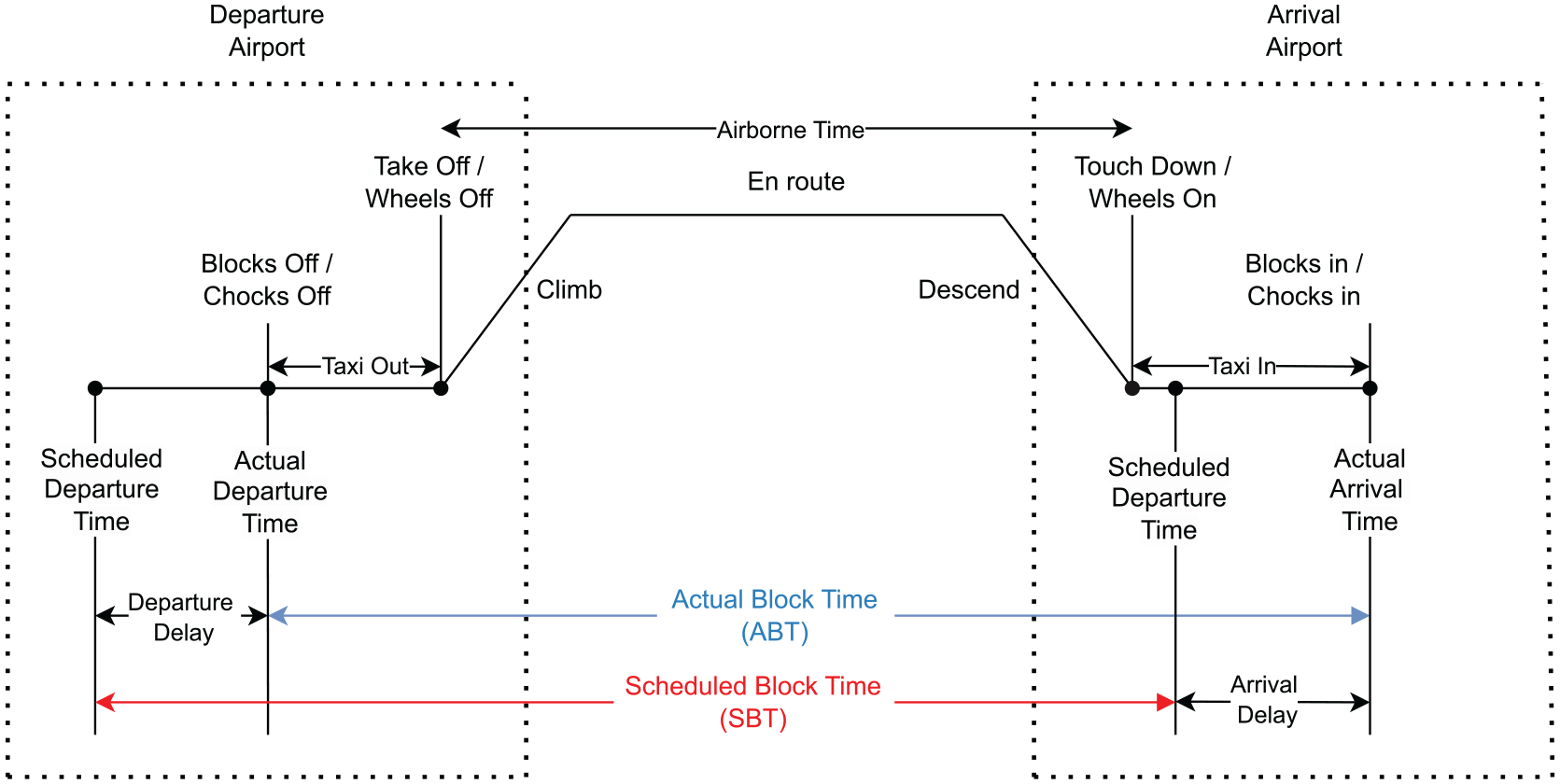
Segments of the flight operations.

Several challenges are encountered in SBT estimation because of the long-term prediction horizon and the dynamic nature of airline operations. Prediction takes place months in advance, making it impossible to accurately anticipate factors such as wind, weather, air traffic, and aircraft load ( 2 – 4 ). As a result, only factors that are known a few months in advance, such as the origin and destination airports, along with time-based features (day, week, month, etc.), can be utilized in any prediction modeling. Moreover, airlines make adjustments closer to flight departure to accommodate real-time changes, and these often go unrecorded. When planning, airlines typically lack information on what affects operations on the actual flight day. This limited availability of explanatory variables in the data makes achieving accurate predictability extremely challenging. Another challenge comes from the nature of the explanatory variables. Many features such as the departure and arrival airports and time-based features are categorical, are of high cardinality, and have spatiotemporal effects that are not well captured by traditional encoding schemes in machine learning. This complexity demands advanced methods for effective modeling and prediction.

Both the over- and underestimation of SBT is undesirable. With a shorter block time, the possibility of delayed arrival arises, leading to disruption of flight sequences, crew displacement, and additional expenses like food and lodging. In contrast, introducing buffers into block time may cause early arrivals, potentially resulting in the inefficient utilization of resources such as crew allocation, thus leading to suboptimal outcomes ( 5 – 8 ). To optimize scheduling and maximize resource utilization, airlines strive to find the most accurate SBT estimate that closely aligns with the ABT.

A broad spectrum of approaches have been employed to estimate flight block times, their components (such as taxi and flight times), and delays. These methodologies range from machine learning techniques, including random forest and XGBoost, to deep-learning models, which have been applied to predict short-term delays ( 9 – 13 ). However, much of this work tends to focus on short-term predictions made typically hours or a day before the day of operations, and it often excludes certain links or routes, suggesting a gap in broader applicability across the airline industry. There is a notable absence in the literature concerning long-term SBT prediction modeling. A recent work by Abdelghany et al. ( 8 ) concluded that machine learning models, specifically regression tree, random forest, and XGBoost, have limited capability in predicting ABT. They show that these models were outperformed by historical median-based estimates of ABT. Moreover, this study only considered a very limited set of routes (seven), which necessitates a large-scale analysis and the investigation and development of more sophisticated neural-network-based approaches for this critical task to effectively exploit the information available at the planning stage and enhance the predictive capabilities of the models.

Adding to the complexity of modeling is the inherent problem with traditional encoding schemes. Although straightforward and commonly used, encoding schemes like one-hot encoding have significant drawbacks. Primarily, since it adds a variable for each unique category of a feature, the model’s dimensionality increases proportionally to the cardinality of the categorical variables. This escalation poses a challenge known as the curse of dimensionality, which demands exponentially more data for the model to remain accurate ( 14 ). Another issue with one-hot encoding is that it assumes that categories are mutually exclusive and unrelated, leading to representations that are orthogonal and equidistant. This fails to capture any natural similarity between categories, overlooking their potential associative or semantic connections ( 15 ). For instance, consider the scenario where we are analyzing a dataset related to days of the month in airline operations. For a human observer, it is clear that the last day of a month and the first day of the following month are close, but once this feature is one-hot encoded we lose this natural progression. Moreover, while circular transformations to encode this closeness between days can be useful, these cannot capture additional complex relationships and similarities. Therefore, learning these latent relationships is key to improving long-term forecasting, especially for a very limited feature set.

To bridge these gaps, our study adopts entity-embedding-based representation learning to discern intricate nonlinear relationships through a neural network framework. Specifically, entity embeddings are task-dependent relationships that the model learns to help the downstream task ( 16 ). This methodology efficiently addresses the challenge of encoding categorical features with high cardinality, a task that is often challenging with traditional encoding schemes. Embedding techniques have significantly evolved to capture complex data relationships in various domains. Starting with RESCAL ( 17 ) and TransE ( 18 ) for knowledge graphs, these methodologies have laid the groundwork for advanced representations. DeViSE ( 19 ) further extended embeddings to map images into semantic spaces. Subsequently, methods like DeepWalk ( 20 ) and Node2Vec ( 21 ) have been developed for graph representations. The most recent work on the use of embeddings for transportation research by Arkoudi et al. ( 22 ) introduces embedding encoding for socio-characteristic variables, aligning latent representations with individuals’ travel behavior choices. This progression highlights the versatility and importance of embedding models in capturing nuanced data relationships across a spectrum of applications.

This study aims to leverage entity-embedding-based representation learning in a neural network to improve flight-scheduling predictions. By learning embeddings, the proposed neural network architecture is intrinsically aware of the task it is being trained for and concurrently learns the multidimensional relationships as the model trains. Henceforth, we refer to entity embeddings ( 16 ) as embeddings, unless otherwise specified. To ensure the robustness of our approach, we conducted ablation studies, leading us to the best-suited neural network architecture. Additionally, we benchmarked our approach against 10 baseline ML models for a thorough comparison using Monte Carlo simulations. Furthermore, we employ t-distributed stochastic neighbor embedding (t-SNE) on the learned embeddings to visualize the high-dimensional representations, revealing patterns learned by the proposed model.

Contributions

1. Entity-embedding-based model. We introduce an entity-embedding-based neural network model for block time prediction, a novel application in aviation analytics for long-term planning.

2. First large-scale study for broader generalization. Unlike the previous studies, which limited their scope to busier links or several airports, our study uses the entire network ( $~6$  million flights across $~5500$ routes), ensuring our model’s generalizability and applicability.

3. Rigorous experimental validation. We rigorously test our model against 10 baseline models using three distinct seeds, ensuring model robustness, reliability, and reproducibility. We also include statistical significance results to further demonstrate the reliability of our model.

4. Ablation studies. To evaluate the utility of each component of the proposed solution on the predictive performance, we conduct extensive ablations across feature compression, embedding integration, dropout, batch normalization, and nonlinearity.

5. Visualization of embeddings. We employ t-SNE to explore the learned entity embeddings and provide insights into the complex relationships learned by the model.

In the sections that follow, we present a literature review on block time and delay prediction, followed by a detailed description of the methodologies applied in this study. Subsequently, we assess the performance of our predictive models and conduct sensitivity analysis.

Literature Review

Through an extensive literature review, we uncovered a diverse range of models that address the estimation of block time, its components (i.e., taxi time, flight time), and delays. While the broader scope of this paper encompasses the long-term prediction of ABT, delays, taxi times, and other related downstream tasks to aid airline operational planning in the long term, our experimental focus and demonstrated results center on the prediction of ABT. In this section, we review the literature on the prediction modeling of time segments of the flight operations, focusing on block time and delay, which seem to have attracted most of the work. We begin by examining the efforts made to estimate block time. Then, we review the modeling of delay propagation and prediction while making the distinction between short-term and long-term prediction.

Block Time Prediction

The prediction of ABT has been the focus of two studies by Wang et al. ( 23 ) and Abdelghany et al. ( 8 ). Wang et al. ( 23 ) proposed a stacking model that demonstrates promising generalization for the prediction of block time for various spatial–temporal instances. Abdelghany et al. ( 8 ) used three machine learning (ML) models—namely, regression tree (RT), random forest regression (RFR), and extreme gradient boosting (XGBoost) regression—to know of when planning their schedules several months in advance. They found that the performance of the ML models was poorer when evaluated against a benchmarking scenario where the median value of historical actual block times was used as an estimate. The analysis employed Bureau of Transportation Statistics (BTS) data from 2019, focusing on seven airport pairs. For the flights along these routes, the study employed outlier filtering by applying a lenient approach using a lower bound =  $Q1-2\times \mathrm{IQR}$ and an upper bound =  $Q3+2\times \mathrm{IQR}$ . Here, $Q1$ represents the first quartile, marking the 25th percentile of the dataset, and $Q3$ represents the third quartile, marking the 75th percentile. $\mathrm{IQR}$ (the interquartile range) is defined as the difference between $Q3$ and $Q1$ , reflecting the middle 50% of the data. This approach has the drawback of eliminating a substantial amount of valuable information, including the crucial tails of the distribution. Their findings indicate that XGBoost outperformed both the RT and RFR models in relation to prediction accuracy. The study identified seasonality, aircraft type, departure/arrival hours, and traffic at the airport as the most influential variables. Furthermore, the study revealed significant variability in actual block time and its components across different airport pairs, with longer routes exhibiting greater variability. It is worth noting that the study’s scope was confined to only seven specific one-way routes, potentially limiting the generalizability of the findings to the broader airline network.

To enhance the understanding of SBT estimation, previous studies have undertaken various analytical approaches. Coy ( 24 ) developed two-stage statistical models corresponding to six U.S. airlines to predict SBT. The approach involved estimating an initial block time by averaging the previous year’s similar flights and using it as a prediction variable in a second-stage regression model. The models are claimed to capture over 95% of the variance, indicating a strong fit. However, their approach relied on a subset of data obtained by dropping the less frequented routes, avoiding the challenges of the long-tailed distribution of block time. In contrast, our approach harnesses the entirety of the data. Moreover, their reliance on variables such as traffic and weather conditions, which are not readily available during the planning phase, potentially limits the practical application of their model for long-term predictions.

Sohoni et al. ( 25 ) note that airlines typically determine SBT based on fixed percentiles of historical data. Expanding on this, Hao and Hansen ( 26 ) suggest that airlines commonly adopt an SBT ranging from the 65th to the 75th percentile of ABT. However, Sohoni et al. ( 25 ) argued that these approaches have not yielded substantial improvements in OTP. Building on this critique, our study introduces a machine learning framework that is not solely dependent on historical trends; it is also capable of learning from available explanatory variables. Deshpande and Arıkan ( 1 ) analyzed flight buffer selection using the newsvendor problem as an analogy, where early or late flight arrivals equate to newspaper vendors experiencing a surplus or shortage. Their study revealed that buffer decisions are notably influenced by carrier types, route market shares, and specific route attributes. Kang and Hansen ( 27 ) modeled how airlines adjust SBT to balance OTP. They analyzed five U.S. domestic airlines and found that schedulers are inclined to extend SBT by $0.38$ to $0.54$  minutes per $1\mathrm{\%}$ rise in OTP. In the same context, Wang et al. ( 4 ) compare the differences in this SBT-setting behavior between major airlines in the U.S. and China. They use econometric models based on historical ABT distributions, the departure delay, as well as other factors that may drive SBTs. They perform counterfactual analysis which indicates that Chinese airlines could attain U.S.-level OTP through U.S. SBT-setting practices, while U.S. airlines might experience slightly lower OTP when using Chinese SBT-setting methods.

Instead of relying on block time prediction, Gui et al. ( 28 ) propose a data-driven three-stage method to enhance the estimation of expected arrival time. Their method involves identifying aircraft arrival patterns (clustering), classification (XGBoost), and estimating flight time (XGBoost). This approach primarily focuses on short-term prediction since it relies on real-time radar trajectory data, including current, historical, and traffic situation information. As a result, it is more suitable for operational use rather than long-term planning, which is the focus of this paper.

Delay Prediction

Flight delay prediction has been extensively researched in the literature ( 29 , 30 ). A significant differentiation can be observed in the practical application of these predictions. In the long term, such predictions are employed for planning and scheduling purposes, including activities like booking slots at the airport, which are done several months in advance of the flight departure. On the other hand, in the short term, predictions are utilized to optimize and enhance the operational efficiency of airlines in real time.

One of the first studies that incorporated the spatiotemporal aspect into the prediction of delay was by Rebollo and Balakrishnan ( 9 ). They defined a NAS (National Airspace System) delay state at time $t$ as a vector of the departure delays of all of the origin–destination (OD) pairs at time $t$ . This delay for an OD pair at time t refers to the median delay of all the flights that fall within a 2-h time window beginning at time $t$ . These NAS delay observations are classified as both a characteristic delay pattern of NAS (i.e., spatial) and a characteristic type of day (temporal). These are then used as explanatory variables which represent the system to predict departure delays using random forests. They evaluated their model on the 100 most delayed links and got an average test error of 20.9 min. Subsequent studies by Gopalakrishnan and Balakrishnan ( 31 ) compared different approaches, including Markov Jump Linear System (MJLS) and artificial neural networks (ANNs), which achieved a 94% accuracy in classifying the 100 delay links with a threshold of 60 min. Our study builds on these insights, targeting a wider scope beyond the 100 most delayed links. Wang and Vaze ( 32 ) model the distribution of primary delays in the NAS, identifying a bimodal pattern with a peak at zero and declining frequency for positive delays, and use a two-phase approach because of quantile regression’s limitations with this distribution. While insightful for delay probabilities, their model does not predict exact delay times for individual flights.

Deep-learning models, on the other hand, have excelled in capturing complex nonlinear relationships in space and time ( 10 , 12 ). Researchers have transformed the multi-airport flight delay prediction into a graph representation learning task ( 13 ). Several other efforts have also been made to develop tree-based and neural network-based models to predict delays at the individual flight, airport, link, and network levels with prediction horizons of minutes, hours, and days ( 10 – 12 ). Another formulation that is frequently seen is the classification problem, which focuses on classifying delay in an OD link, departure/arrival at an airport, or individual flights based on predetermined delay thresholds. Alonso and Loureiro ( 33 ) define the intervals as $(-\infty ,0)$ , $[0,15)$ , $(15,30]$ , $(30,60]$ , $\mathrm{and}(60,\infty )$ . The idea here is to assign delays to one of these severity levels, allowing for a more detailed understanding of delay patterns and their influence on operations.

Interestingly, most of the research around delay prediction has been restricted to the last hours or days before departure, when data sources are abundant. For example, weather data and information on the state of the airline network, both strongly associated with delay, are typically used. However, in a long-term context, only a couple of studies have addressed this challenge. Lambelho et al. ( 34 ) proposed a generic approach to assess strategic flight schedules (arrival/departure slots several months before execution) based on flight delay and cancellation predictions. Their analysis showed that LightGBM outperformed other models in delay prediction, emphasizing key factors like airlines and seats in forecasting arrival delay with high accuracy and Area under the curve (AUC) metrics. Kafle and Zou ( 7 ) presented an analytical model to quantify the propagated and newly formed delays. Wong and Tsai ( 6 ) used survival analysis to find key contributing factors for departure and arrival delays. Their results indicate that key factors affecting departure delays include turnaround buffer time, aircraft type, logistics, and weather, while arrival delays are primarily influenced by block buffer time and weather conditions.

Proposed Approach

Our objective is to develop a predictive model equipped to process high-dimensional categorical variables and intricate relationships between them for predicting delays, block time, taxi-in and taxi-out times, and other critical operational parameters. The predictive model for such tasks can be formulated the bold variables are vectors as

$$y=f({\mathit{x}}^{\mathrm{cat}},{\mathit{x}}^{\mathrm{cont}})$$

(1)

where $y\in \mathbb{R}$ represents the outcome of interest (e.g., block time, but this can be the delay time, taxi-out time, etc. for other applications); $f(·)$ is the predictive function; ${\mathit{x}}^{\mathrm{cont}}\in {\mathbb{R}}^{n_{\mathrm{cont}}}$ denotes the vector for continuous features pertinent to the downstream prediction tasks, where $n_{\mathrm{cont}}$ is the total number of continuous variables; and ${\mathit{x}}^{\mathrm{cat}}\in {\mathbb{R}}^{n_{\mathrm{cat}}}$ denotes the vector for the categorical features. Note that we are not modeling a time-series dataset and only use static flight characteristics.

The features ${\mathit{x}}^{\mathrm{cat}}$ and ${\mathit{x}}^{\mathrm{cont}}$ constitute the features influencing the outcome $y$ . Some of these are deterministic and well understood, yet many exhibit intricate relationships that are nondeterministic and less apparent; specifically:

• Temporal variations. Seasonal factors, like snow, may lead to longer block times because of requirements like deicing. Weekends or peak travel times might exacerbate taxi times because of congestion.

• Airline-specific practices. Different carriers maintain distinct operational philosophies. An airline might value quick turnarounds, optimizing for reduced block times, while another could emphasize longer layovers to ensure a buffer against disruptions.

The nondeterministic nature of these factors presents challenges when incorporating domain expertise into prediction models. To effectively capture these multifaceted interactions, we undertake a representation learning task.

To leverage the latent information encoded within the data, we enrich our feature set by learning the embedding ( 16 ) ${\mathit{z}}_i$ from the categorical variables $x_i^{\mathrm{cat}}$ . To this end, we first represent $x_i^{\mathrm{cat}}$ as its one-hot encoded counterpart ${\mathit{v}}_i^{\mathrm{cat}}$ (of dimensions commensurate with the categorical values $x_i^{\mathrm{cat}}$ can take). For instance, if the feature $x_i^{\mathrm{cat}}$ can take $m_i$ unique categorical values, then ${\mathit{v}}_i^{\mathrm{cat}}\in {\mathbb{R}}^{m_i}$ is a vector of zeros except for a $1$ at the location corresponding to the value $x_i^{\mathrm{cat}}$ .

Now, introducing ${\mathit{v}}_i^{\mathrm{cat}}$ , we obtain the representation ${\mathit{z}}_i=g_i\left({\mathit{v}}_i^{\mathrm{cat}}\right)$ , where $g_i(·)$ is the embedding function and ${\mathit{z}}_{\mathrm{i}}\in {\mathbb{R}}^{d_i}$ is the embedding of the $i^{\mathrm{th}}$ categorical feature. The role of the embedding function $g_i(·)$ is critical. It maps each level of the categorical variable $x_i^{\mathrm{cat}}$ to a low-dimensional parameter vector. Embedding functions are typically linear mappings which can be represented by an embedding matrix ${\mathit{G}}_i$ as

$${\mathit{z}}_i={\mathit{v}}_i^{\top }·{\mathit{G}}_i$$

(2)

Given this, we train a mapping $f(·)$ (a neural network in this case) as

$$y=f\left({[{\mathit{x}}^{\mathrm{cont}},{\mathit{z}}_1,{\mathit{z}}_2,\dots ,{\mathit{z}}_{n_{\mathrm{cat}}}]}^{\top }\right)$$

(3)

The action of the first layer of such a neural network can be written as follows (see also Figure 2):

$${\mathit{h}}_0=\sigma ({\mathit{W}}_1·{\mathit{x}}_0+b_1),\mathrm{for}{\mathit{x}}_0=[{\mathit{z}}_1;{\mathit{z}}_2;\dots ;{\mathit{z}}_{n_{\mathrm{cat}}};{\mathit{x}}^{\mathrm{cont}}]$$

(4)

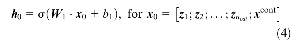
Here, the function $\sigma$ denotes the activation function, which can be any nonlinear function (like the sigmoid, tanh, or Rectified Linear Unit (ReLU) function) that introduces nonlinearity into the model. Note that the embedding matrix ${\mathit{G}}_i$ is jointly optimized with the parameters of the neural network $f(·)$ via backpropagation, as depicted in Figure 2. This helps us to extract customized representations of input categorical variables to achieve optimal performance for the given task.

Figure 2.

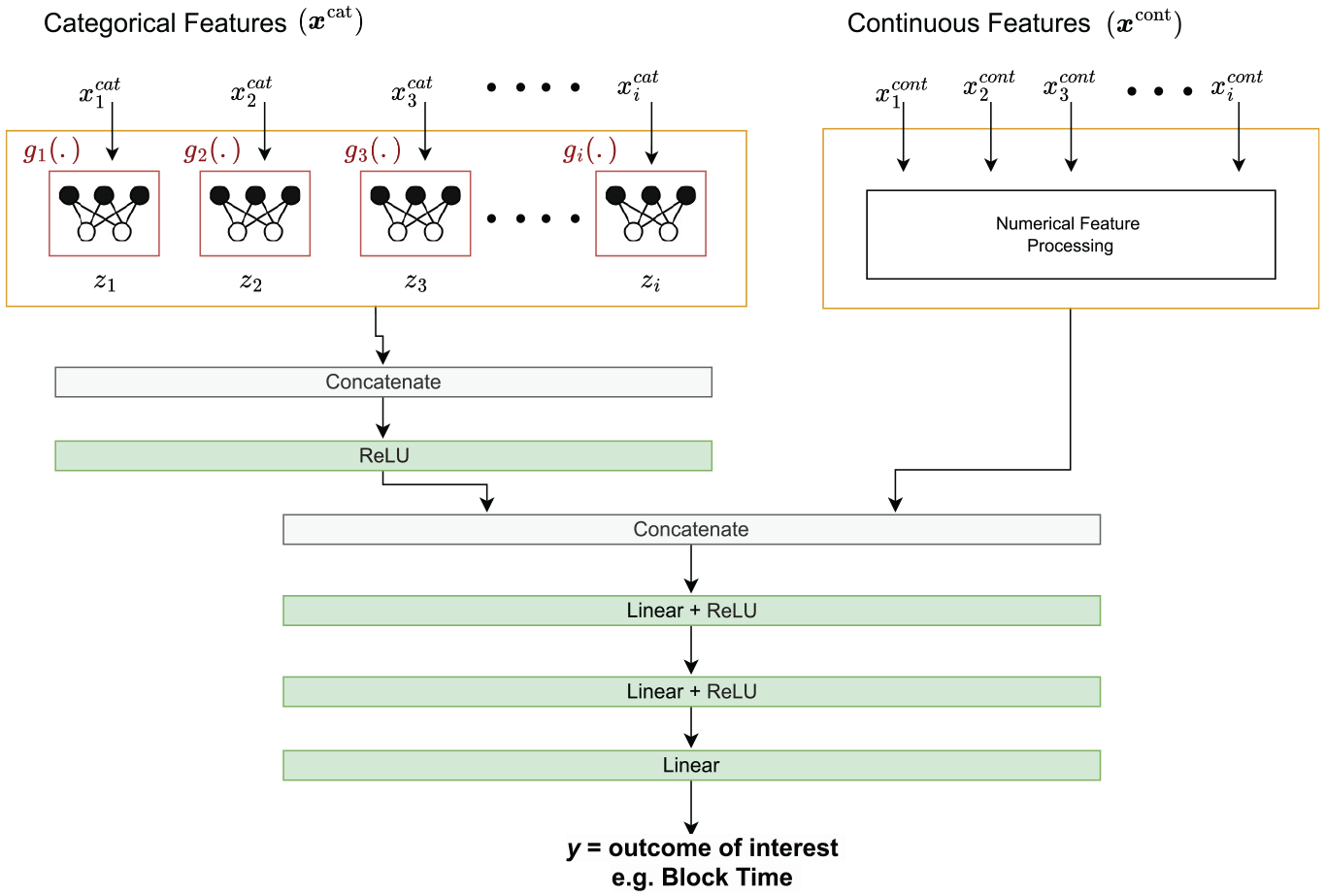
Block diagram: harnessing categorical embeddings and continuous features for specific tasks.

Experiments

This section outlines the dataset, the preprocessing steps, the baseline models used for comparison, and the various neural network architectures explored in our study.

Data Overview

The data used for this study were obtained from the airline on-time performance database. This database comprises scheduled actual departure and arrival times recorded by certified U.S. air carriers, which account for a sizable share of the domestic scheduled passenger revenue. This database is compiled by the Office of Airline Information of the Bureau of Transportation Statistics (BTS). It provides complete details on on-time arrival and departure dates, flight cancellations and diversions, taxi-out and taxi-in times, causes of delay and cancellation, air times, and non-stop distances.

For the purpose of block time prediction, we use the 2018 data, comprising more than 6 million flights operated by 17 airlines. Table 1 provides a detailed breakdown of each airline’s percentage of short-, medium-, and long-haul flights based on block time alongside their International Air Transport Association (IATA) code, names, regional or international classification (R/I), and operational model (HS or P2P). The table is sorted in decreasing order of the percentage of short-haul flights (%S).

Table 1.

Airlines and Their Percentages of Short-Haul (%S; <3 h), Medium-Haul (%M; 3–6 h), and Long-Haul (%L; >6 h) Flights in 2018, Based on Block Time (Airlines Are Sorted in Decreasing Order of %S)

IATA code	Airline name	R/I	OM	%S	%M	%L
OH	PSA	R	HS	99.5	0.5	0.0
MQ	American Eagle	R	HS	97.9	2.1	0.0
EV	ExpressJet	R	HS	97.6	2.4	0.0
9E	Pinnacle	R	HS	95.8	4.2	0.0
YV	Mesa	R	HS	91.8	8.2	0.0
OO	SkyWest	R	HS	91.5	8.5	0.0
YX	Midwest	R/I	HS	89.3	10.7	0.0
WN	Southwest	R/I	P2P	85.0	14.9	0.1
HA	Hawaiian	I	HS	79.8	15.2	5.0
DL	Delta	I	HS	75.2	23.4	1.4
NK	Spirit	R/I	P2P	69.9	29.8	0.4
B6	JetBlue	R/I	P2P	68.5	27.5	4.0
F9	Frontier	R/I	P2P	68.2	31.7	0.1
AA	American	I	HS	65.2	32.6	2.3
UA	United	I	HS	58.2	38.3	3.5
AS	Alaska	I	HS	53.8	39.0	7.2
VX	Virgin America	I	HS	44.5	41.8	13.7

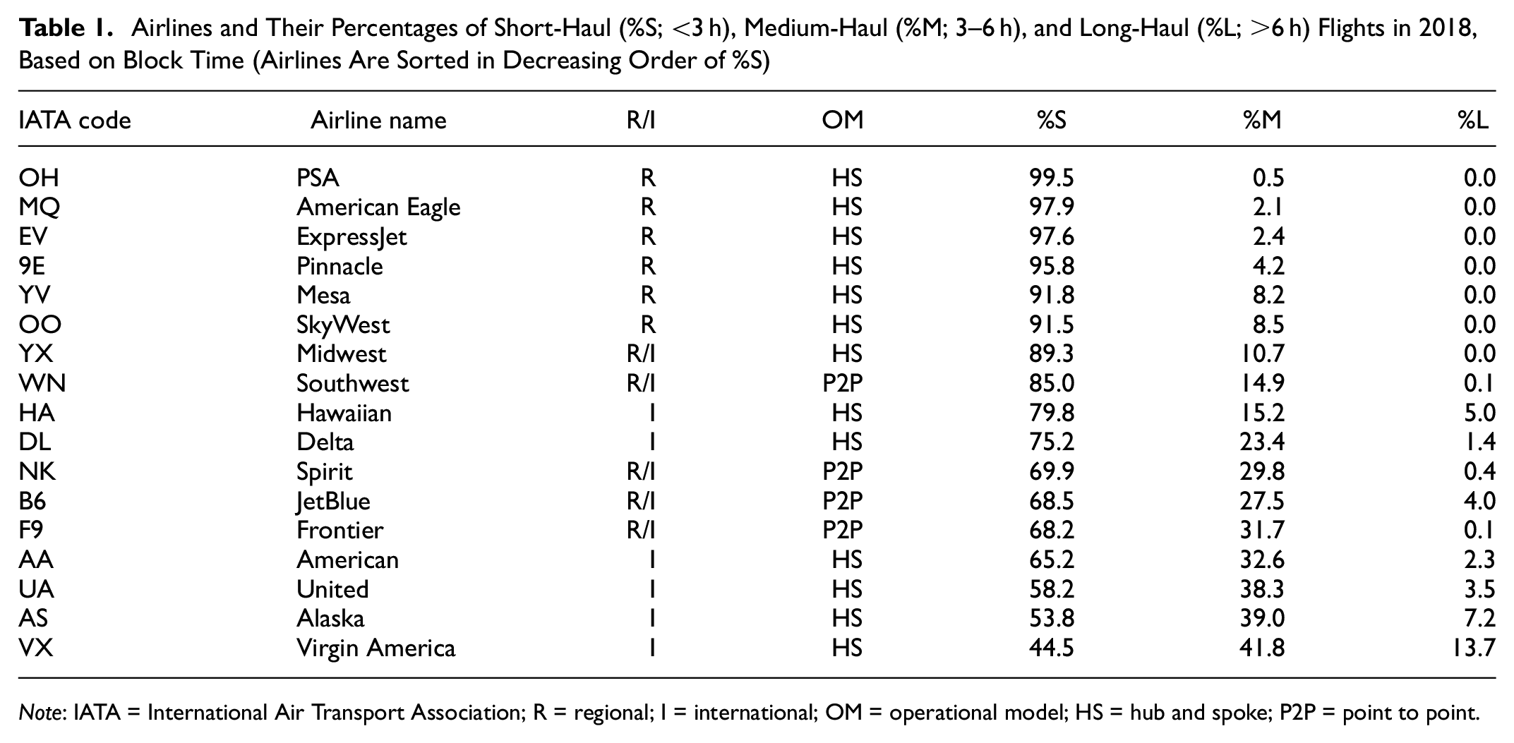
Note: IATA = International Air Transport Association; R = regional; I = international; OM = operational model; HS = hub and spoke; P2P = point to point.

Figure 3 provides a comprehensive visualization of the ABT distributions. The primary plot at the top of the grid depicts the overall distribution across all airlines, revealing a right-skewed pattern with a pronounced long tail. The subsequent plots, each labeled with an IATA code, represent the block time distributions of 17 individual airlines. The differences in these distributions are quite pronounced, reflecting the varied operational profiles of the airlines as described in Table 2. Some airlines, potentially those servicing shorter routes, showcase a more centered distribution, while others exhibit broader spreads, suggesting a mix of short- and long-haul flights. For instance, regional airlines like ExpressJet Airlines (EV) often operated multiple short hops per day, where delays can accumulate with each subsequent flight. In contrast, medium- and long-haul flights operated by airlines such as Alaska Airlines (AS) experience more variability from weather conditions, such as sustained headwinds at cruise altitudes. Additionally, Figure 4 illustrates the block time variation across the top 10 busiest origin–destination (OD) pairs, highlighting the variability that occurs not only across routes but also within each route and arises from the operating conditions, different airline practices, and other factors, further emphasizing the complex nature of predicting block times accurately.

Figure 3.

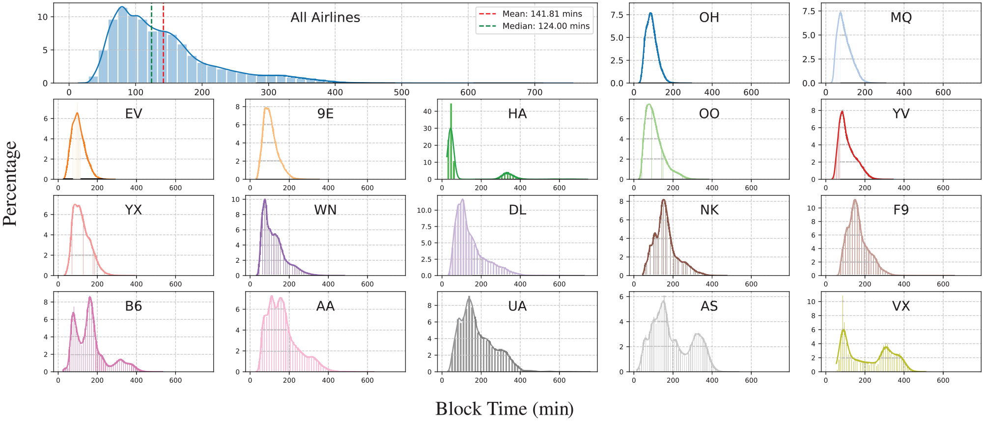
Block time (ABT) distributions for 2018. The main plot illustrates the aggregate distribution, while individual subplots capture airline-specific variations denoted by International Air Transport Association codes. The plots are sorted in decreasing order of %S (% short-haul flights) by airline.

Table 2.

List of Variables

Sr. no.	Variable	Type	Nature
1	Quarter	Categorical	Temporal
2	Month	Categorical	Temporal
3	DayofMonth	Categorical	Temporal
4	DayOfWeek	Categorical	Temporal
5	Reporting_Airline	Categorical	-
6	OriginAirportSeqID	Categorical	Spatial
7	Origin	Categorical	Spatial
8	DestAirportSeqID	Categorical	Spatial
9	Dest	Categorical	Spatial
10	Weekend	Categorical	Temporal
11	IATASeason	Categorical	Temporal
12	FlightSequenceTails	Numerical	-
13	sin_CRSDepTime	Numerical	Temporal
14	cos_CRSDepTime	Numerical	Temporal
15	sin_CRSArrTime	Numerical	Temporal
16	cos_CRSArrTime	Numerical	Temporal
17	OriginLongitude	Numerical	Spatial
18	OriginLatitude	Numerical	Spatial
19	DestLongitude	Numerical	Spatial
20	DestLatitude	Numerical	Spatial
21	Distance	Numerical	Spatial
22	CRSElapsedTime	Numerical	Temporal

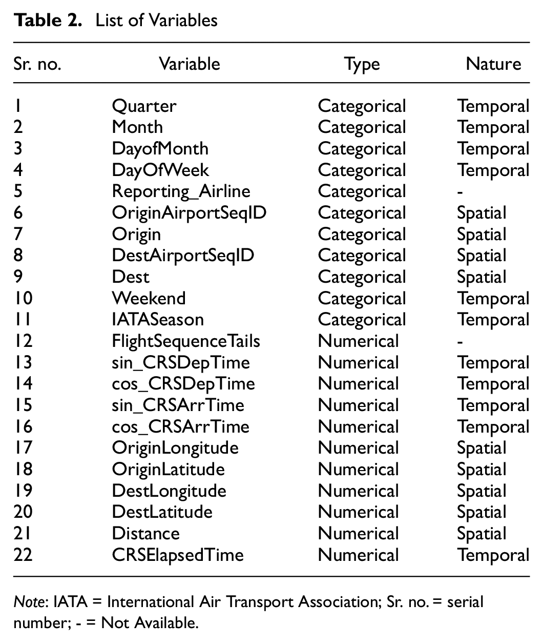
Note: IATA = International Air Transport Association; Sr. no. = serial number; - = Not Available.

Figure 4.

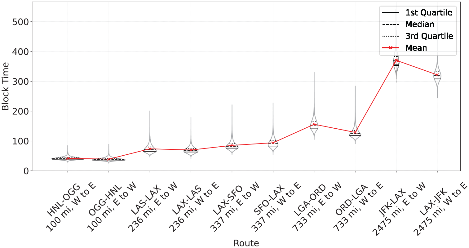
Block time (ABT) variations across the top 10 busiest links (sorted by the distance between the origin and destination airports). Violin plots depict block time variations for the 10 busiest routes (with internal lines indicating quartiles and means), showcasing the within-route variability and providing comparisons across routes.

Data Pre-Processing

Accurately capturing the periodic nature of temporal attributes is critical for modeling the nuances of airline operations. These patterns, especially in the context of timestamps like CRSArrTime and CRSDepTime, influence metrics like block times in airline operations. Table 3 provides comprehensive summary statistics of the temporal categorical features, highlighting the variability of ABT for flights across different time frames. To encode the cyclical pattern in time, we circularly transformed timestamps through the application of sine and cosine functions, enabling them to be represented as angles within a circular space. This approach ensures continuity between the endpoints of a cycle, allowing the subsequent models to recognize and leverage these cyclical dependencies. Recognizing the interdependencies of flights in a sequence and to capture the compounding delays, we also introduce FlightSequenceTails, which is a numerical attribute that encodes the order of flights based on their flight dates and tail numbers, providing insights into the cascading delays.

Table 3.

Summary Statistics Across Temporal Categorical Features

Category	Number of flights (%)	Actual block time (ABT; min)
		Mean	SD	Minimum	Maximum	Median
Quarter
1	1274079 (21.46)	145.98	77.14	16	739	129
2	1394307 (23.49)	145.72	77.43	14	757	128
3	1567716 (26.41)	140.98	75.81	15	736	122
4	1700866 (28.65)	136.23	72.75	14	723	117
Month
January	459645 (7.74)	142.31	75.52	16	728	125
February	374254 (6.30)	148.33	78.34	16	739	132
March	440180 (7.41)	147.83	77.63	16	711	132
April	490286 (8.26)	142.05	75.84	16	757	124
May	451195 (7.60)	146.97	78.05	16	717	129
June	452826 (7.63)	148.45	78.35	14	680	131
July	469832 (7.91)	149.08	78.71	16	736	132
August	542624 (9.14)	140.93	76.02	16	681	122
September	555260 (9.35)	134.18	72.35	15	689	115
October	586714 (9.88)	134.04	72.02	14	684	115
November	554906 (9.35)	136.26	72.51	17	704	118
December	559246 (9.42)	138.51	73.67	17	723	120
DayofMonth
1	190670 (3.21)	142.32	76.28	16	711	124
2	191264 (3.22)	142.06	76.28	17	757	124
3	187919 (3.17)	142.20	76.26	16	717	124
4	190092 (3.20)	140.68	75.48	17	694	122
5	197608 (3.33)	140.74	75.48	16	728	122
6	193019 (3.25)	141.90	75.98	17	705	124
7	193890 (3.27)	142.00	75.99	15	723	124
8	193516 (3.26)	141.63	75.67	16	718	123
9	197497 (3.33)	142.04	75.27	16	699	124
10	193379 (3.26)	141.74	75.36	18	692	124
11	197560 (3.33)	141.66	75.55	17	690	123
12	200615 (3.38)	141.33	75.10	16	705	123
13	194056 (3.27)	141.62	75.42	17	697	123
14	193841 (3.26)	141.97	75.58	16	684	124
15	192032 (3.23)	143.43	76.36	14	736	125
16	198422 (3.34)	141.56	75.57	16	739	123
17	193884 (3.27)	141.73	75.62	17	701	124
18	198076 (3.34)	140.62	75.16	16	728	122
19	201924 (3.40)	141.29	75.51	16	704	123
20	196443 (3.31)	142.97	76.11	16	691	125
21	195247 (3.29)	142.29	75.67	14	696	124
22	189929 (3.20)	142.28	76.22	17	711	124
23	196369 (3.31)	141.16	75.51	17	698	123
24	195446 (3.29)	141.55	75.61	16	693	123
25	196821 (3.32)	142.00	75.85	17	700	124
26	201084 (3.39)	142.19	75.84	16	711	124
27	193075 (3.25)	142.09	75.88	17	708	124
28	194765 (3.28)	142.47	75.80	18	712	124
29	183566 (3.09)	141.29	75.59	17	714	123
30	186109 (3.13)	140.68	75.31	17	704	122
31	108850 (1.83)	143.23	76.77	18	693	125
DayOfWeek
Monday	892504 (15.03)	141.52	75.49	14	757	123
Tuesday	850995 (14.33)	140.53	75.17	16	699	122
Wednesday	861131 (14.50)	140.70	75.26	16	711	122
Thursday	872859 (14.70)	141.91	75.91	14	725	123
Friday	880776 (14.84)	141.77	75.81	15	739	123
Saturday	733982 (12.36)	144.25	76.58	16	714	127
Sunday	844721 (14.23)	142.35	75.97	16	736	124
Weekend
No	4358265 (73.41)	141.29	75.53	14	757	123
Yes	1578703 (26.59)	143.23	76.26	16	736	126
IATASeason
Winter	2357187 (39.7)	141.42	75.21	16	739	123
Summer	3579781 (60.3)	142.06	76.07	14	757	124

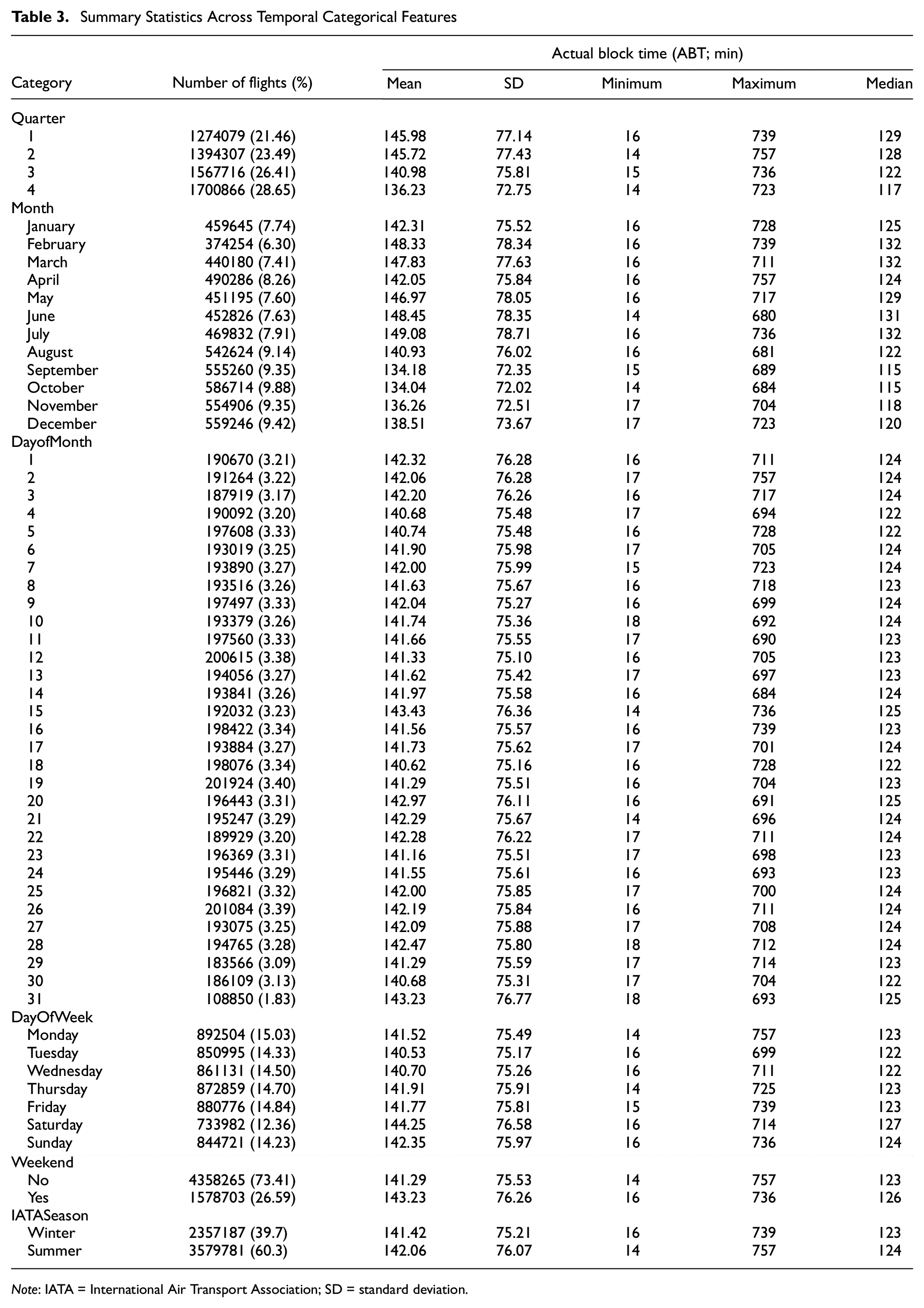
Note: IATA = International Air Transport Association; SD = standard deviation.

Baseline Models

In predictive modeling, especially when dealing with tabular datasets comprising categorical and continuous features, the choice of algorithm plays a pivotal role in predictive performance. Our choice of baseline models reflects a spectrum of algorithms that have traditionally demonstrated robust performance on tabular data, and they were selected to encompass both linear and nonlinear complexities inherent to the data ( 35 – 41 ). Additionally, these models range from ones that directly handle regularization to counteract potential overfitting to the ensemble and boosting methods known for their high accuracy in diverse scenarios. The models presented in Table 4 were considered.

Table 4.

Baseline Models

Model	Description
Linear	Linear without any regularization
Lasso	Linear with L1 regularization
Ridge	Linear with L2 regularization
Elastic net	Linear with both L1 and L2 regularization
Decision tree	Nonlinear with a single tree
Random forest	Ensemble of decision trees
HGBoost	Gradient boosting with histogram-based trees
XGBoost	Tree-based gradient boosting with level-wise growth
LightGBM	Tree-based gradient boosting with leaf-wise growth
AdaBoost	Boosting with multiple weak learners

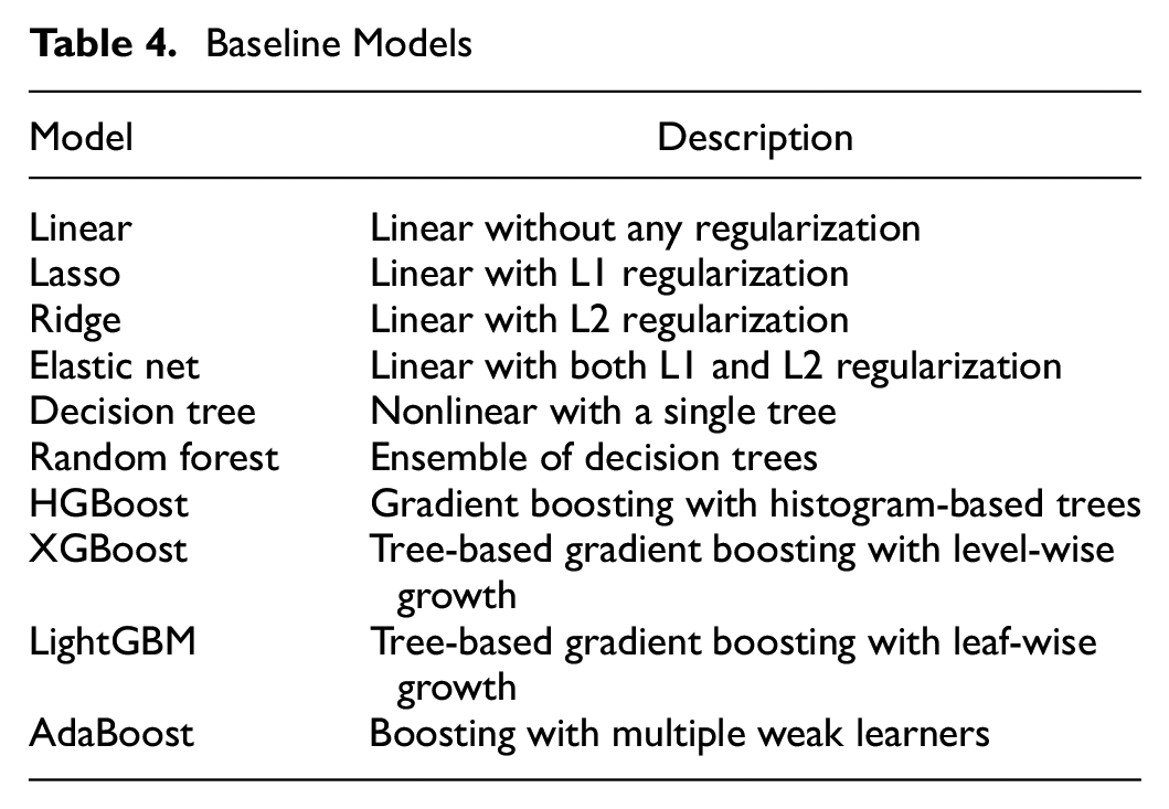
For handling the categorical features, one-hot encoding is employed. In the context of generalized linear models (GLMs), this encoding allows each category to be treated distinctly, with models fitting specific coefficients for each category. For tree-based models, the encoding directly affects the decision-making process. Tree splits will be determined based on the presence or absence of the encoded categorical variables, thus influencing how the model interprets and acts on the data. Having experimented with the traditional modeling approaches, we now set our sights on the vast potential of neural-network-based architectures.

Neural Network (NN) Architectures

Baselines Using One-Hot Encoding NN_OHE_25

We analyze various configurations of neural network architectures. First, we consider architectures that do not include an embedding layer. For these models, we begin with one-hot encodings of the categorical variables as described in the “Proposed Approach” section, and we directly feed these into the neural network without the embedding layer for the categorical variables. Since the embedding layer is a linear layer, we also choose this to be a linear layer for a fair comparison. Here, the dimension that the first layer maps to becomes an important parameter. To analyze the impact of compression caused by the action of the first layer, we analyze the following variants.

NN_OHE_25

This variant introduces a compression to keep $75\mathrm{\%}$ of the input dimensions (i.e., a 25% compression). Formally for each categorical variable $x_i^{\mathrm{cat}}$ , we obtain the corresponding one-hot encoding ${\mathit{v}}_i^{\mathrm{cat}}$ as described in the “Proposed Approach” section and then concatenate all one-hot encoded categorical representations to form ${\mathit{x}}_{\mathrm{ohe}}$ as

$$\begin{array}{c}{\mathit{x}}_{\mathrm{ohe}}=[{\mathit{v}}_1^{\mathrm{cat}};{\mathit{v}}_2^{\mathrm{cat}};\dots ;{\mathit{v}}_{n_{\mathrm{cat}}}^{\mathrm{cat}}]\hfill \\ \multicolumn{1}{c}{{\mathit{x}}_{\mathrm{lin}}={\mathit{W}}_{\mathrm{cat}}{\mathit{x}}_{\mathrm{ohe}}+b_{\mathrm{cat}}}& \hfill & \hfill \end{array}$$

where ${\mathit{W}}_{\mathrm{cat}}$ and $b_{\mathrm{cat}}$ are the parameters of the linear layer. The following concatenated representation integrates the continuous features:

$$\begin{array}{ccc}\mathit{x}=[{\mathit{x}}_{\mathrm{lin}};{\mathit{x}}_{\mathrm{cont}}]\hfill & \hfill & \hfill \end{array}$$

(5)

Then, $\mathit{x}$ is transformed using two fully connected layers as

$$\begin{array}{ccc}{\mathit{h}}_0=\sigma ({\mathit{W}}_1\mathit{x}+b_0)\mathrm{and}{\mathit{h}}_1=\sigma ({\mathit{W}}_2{\mathit{h}}_0+b_1)\hfill & \hfill & \hfill \end{array}$$

(6)

where ${\mathit{h}}_0$ and ${\mathit{h}}_1$ are the outputs of the first and second fully connected layers, respectively. Finally, the output $o$ is computed as

$$\mathrm{o}={\mathit{W}}_3{\mathit{h}}_1+b_2$$

(7)

where ${\mathit{W}}_1,{\mathit{W}}_2,\mathrm{and}{\mathit{W}}_3$ are weight matrices and $b_0,b_1,\mathrm{and}{b}_2$ capture the bias corresponding to each layer.

NN_OHE_50

Building on NN_OHE_25, we experimented with a more aggressive compression strategy, retaining 50% of the initial dimensions after one-hot encoding. The objective was to extract crucial features.

Using embeddings

Embeddings provide a dense representation of categorical variables. Instead of using a sparse matrix as in one-hot encoding, embeddings map each category to a point in a continuous vector space. This allows the model to place similar categories closer together, learning the relationships between categories during training.

NN_EMB

Drawing inspiration from the structure set by the NN_OHE _50 architecture, where categorical data were initially represented using one-hot encoding, in NN_EMB_D_B, we pivot to a more sophisticated approach by replacing the one-hot encoded layer with an embedding layer. Given the input feature vector, ${\mathit{x}}^{\mathrm{cat}}$ and ${\mathit{x}}^{\mathrm{cont}}$ for categorical and continuous variables, respectively, we obtain the embeddings ${\mathit{z}}_i$ for each categorical variable $x_i^{\mathrm{cat}}$ as described in the “Proposed Approach” section. The obtained embeddings are concatenated and then passed through a ReLU layer to introduce nonlinearity, after which they are concatenated with continuous features to form ${\mathit{x}}_0$ , as shown in Equation 4; the overall procedure is shown in Figure 2. Then it is passed through two fully connected layers, as in Equation 6, with the input being ${\mathit{x}}_0$ .

NN_EMB_CORE

Expanding on the NN_EMB framework, this architecture introduces two key modifications: batch normalization and dropout layers. These changes are aimed at optimizing the learning process and enhancing the model’s generalization capabilities.

NN_EMB_D_B

This architecture removes the nonlinearity immediately following the embedding layer in NN_EMB_CORE. This approach is used to ascertain if the initial nonlinearity was perhaps preemptively capturing or distorting the relationships within the data.

Evaluation Metrics

The primary metric used for the evaluation of model performance is the root mean square error (RMSE), defined as

$$RMSE=\sqrt{\frac{1}{n}\sum _{i=1}^n{\left(y_i-{\hat{y}}_i\right)}^2}$$

(8)

where $y_i$ , and ${\hat{y}}_i$ are the actual and the predicted block times, respectively, and $n$ is the number of observations. This choice aligns with the precedent set by notable studies in the field ( 9 , 10 , 13 , 42 , 43 ), which also employed the RMSE to gauge the prediction accuracy in airline operations and delays.

Further, to ascertain the statistical significance of the differences observed in the performance of the multiple models, an analysis of variance (ANOVA) was employed. We make use of p-values and confidence intervals to determine whether the observed differences could have occurred by chance, with p-values below 0.05 indicating statistically significant differences.

In addition to the RMSE, the mean absolute error (MAE) was utilized for the sensitivity analysis. This is defined as

$$\mathrm{MAE}=\frac{1}{n}\sum _{i=1}^n|y_i-{\hat{y}}_i|$$

(9)

Unlike the RMSE, the MAE does not square the errors, thus providing a direct average error magnitude without unduly penalizing larger errors. This metric is useful for evaluating model performance in practical scenarios, reflecting the operational impact of prediction inaccuracies.

Results and Discussion

In this section, we present and discuss the results of block time prediction models. Both the baselines and the neural network models were subjected to an identical experimental framework. The data were distributed into training, validation, and testing subsets, taking 64%, 16%, and 20% of the total, respectively. Each model underwent training, validation, and testing across three distinct random seeds.

Comparing Baselines and Neural Networks

Table 5 presents the comparative performances of the baseline models and neural network architectures. The methods can be categorized into three distinct clusters: traditional regression approaches, tree-based algorithms, and neural-network-based models. Linear, lasso, and ridge regressions display nearly identical performances with minimal variations. The elastic net, while similar, shows slightly poorer performance and greater variability. This is reflected in their test error confidence intervals (CIs), which overlap, as shown in Figure 5. Conversely, the decision-tree and random-forest CIs overlap, indicating similar performances, as do the CIs for HGBoost, LightGBM, and XGBoost. However, NN_EMB’s CI does not overlap with those of the other models, suggesting its performance differs significantly.

Table 5.

Test Performance Comparisons (Each Test RMSE Represents the RMSE for the Best Set of Hyperparameters, Averaged Across Three Distinct Random Seeds)

Model name	Test RMSE in min (SD)
Baseline traditional regression
Linear	13.359 (0.011)
Lasso	13.360 (0.011)
Ridge	13.359 (0.011)
Elastic net	13.407 (0.026)
Baseline tree-based models
Decision tree	13.880 (0.010)
Random forest	13.834 (0.014)
HGBoost	12.891 (0.039)
LightGBM	12.875 (0.003)
AdaBoost	16.362 (0.290)
XGBoost	12.847 (0.046)
Neural networks
NN_OHE_25	20.651 (14.543)
NN_OHE_50	12.622 (0.027)
NN_EMB_D_B	13.211 (0.218)
NN_EMB_CORE	13.556 (0.452)
NN_EMB	11.273 (0.022)

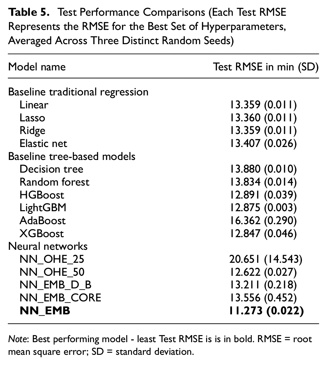
Note: Best performing model - least Test RMSE is is in bold. RMSE = root mean square error; SD = standard deviation.

Figure 5.

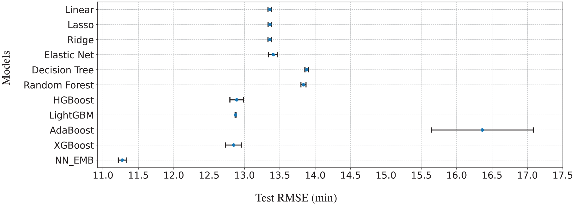
Confidence intervals of test RMSEs for the baseline models and NN_EMB. The blue markers on the graph show the average test RMSEs of the models, while the error bars indicate their 95% confidence intervals.

On the neural network front, both NN_EMB and NN_OHE_50 consistently outperform all the baseline models. It is evident that NN_EMB holds a distinct edge over NN_OHE_50. With a test RMSE of 11.273 min, it not only yields a better prediction accuracy compared with the 12.622 min of NN_OHE_50 but also less variation in performance. Figure 7 compares the train and test performance across baselines and neural networks based models. Consequently, we select NN_EMB as the optimal neural architecture for benchmarking against the baseline models.

To determine the statistical significance of the improvement in prediction error by NN_EMB, an ANOVA was conducted. This ANOVA compared the test RMSE across 10 baseline models and NN_EMB. The results revealed a significant effect of the model on the test RMSE (F-statistic(10, 22) = 535.55, p < 0.0001), indicating marked differences in performance among the evaluated models. On confirming significant differences, Tukey’s Honestly Significant Difference (HSD) post-hoc analysis was applied to perform pairwise comparisons of the means, with the family-wise error rate (FWER) controlled at 0.05. Table 6 details these comparisons, presenting the differences in the mean ( $\mathrm{\Delta }$ Mean) of the test RMSE across seeds, the 95% confidence interval for each difference, and the adjusted p-value (Adj. P) for statistical significance. Given that the adjusted p-value is less than 0.05, we can conclude with 95% confidence that the differences in mean test RMSE between all baseline models and NN_EMB are statistically significant.

Table 6.

Tukey HSD Post-Hoc Comparisons Based on Mean Test RMSE Differences, 95% CIs, and Adj. P Values, Which Affirm the Statistical Significance of NN_EMB’s Performance Over the Baselines

Comparison	$\mathrm{\Delta }$ Mean	95% CI	Adj. P
Versus linear	2.087	(1.823, 2.350)	<0.0001
Versus lasso	2.088	(1.824, 2.351)	<0.0001
Versus ridge	2.087	(1.823, 2.350)	<0.0001
Versus elastic net	2.134	(1.870, 2.398)	<0.0001
Versus decision tree	2.607	(2.343, 2.871)	<0.0001
Versus random forest	2.562	(2.298, 2.825)	<0.0001
Versus HGBoost	1.618	(1.355, 1.882)	<0.0001
Versus LightGBM	1.602	(1.338, 1.866)	<0.0001
Versus AdaBoost	5.089	(4.826, 5.353)	<0.0001
Versus XGBoost	1.575	(1.311, 1.838)	<0.0001

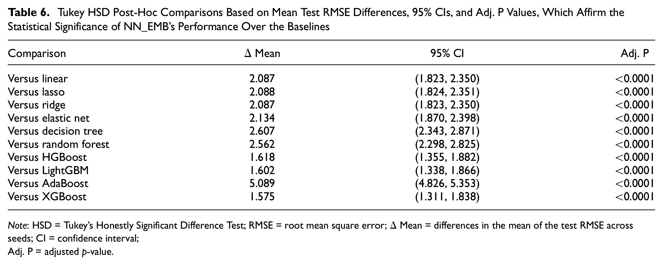
Note: HSD = Tukey's Honestly Significant Difference Test; RMSE = root mean square error; $\mathrm{\Delta }$ Mean = differences in the mean of the test RMSE across seeds; CI = confidence interval; Adj. P = adjusted p-value.

The better performance of NN_EMB can be attributed to the utilization of embeddings, particularly when tasked with encapsulating features of high cardinality. Traditional encoding schemes often struggle in this regard. Techniques such as one-hot encoding, for instance, operate under the assumption that each category is independent of others, suggesting no inherent similarity between varying categories. This can often be a simplistic and inaccurate representation, as it assumes categories to be orthogonal. Another notable advantage of using embeddings is the adaptability they offer. For instance, if a new airport is incorporated into the dataset, the learned embeddings can be fine-tuned to accommodate these new data, ensuring model robustness and adaptability.

Performance Evaluation and Ablations

We performed a series of modifications of the initial model, employing One-Hot Encoding (OHE) and 25% compression to understand the effects of adding, removing, and replacing elements of the architectures. The outcomes of these variations are summarized in Table 7. It is worth noting that the initial performance of NN_OHE_25 improves significantly when retaining only 50% of the initial dimensions after one-hot encoding. NN_OHE_50 focuses on more critical features, thereby reducing noise and improving performance.

Table 7.

Overview of Architecture Modifications (Each Test RMSE Represents the RMSE for the Best Set of Hyperparameters, Averaged Across Three Distinct Random Seeds)

Name	Modifications	Test RMSE in min (SD)
NN_OHE_25	Initial (OHE with 25% compression)	20.651 (14.543)
NN_OHE_50	$\mathrm{\Delta }$ 50% compression	12.622 (0.027)
NN_EMB	$\mathrm{\Delta }$ embeddings	11.273 (0.022)
NN_EMB_CORE	+ dropouts + batch norms	13.556 (0.452)
NN_EMB_D_B	− ReLU after embedding	13.211 (0.218)

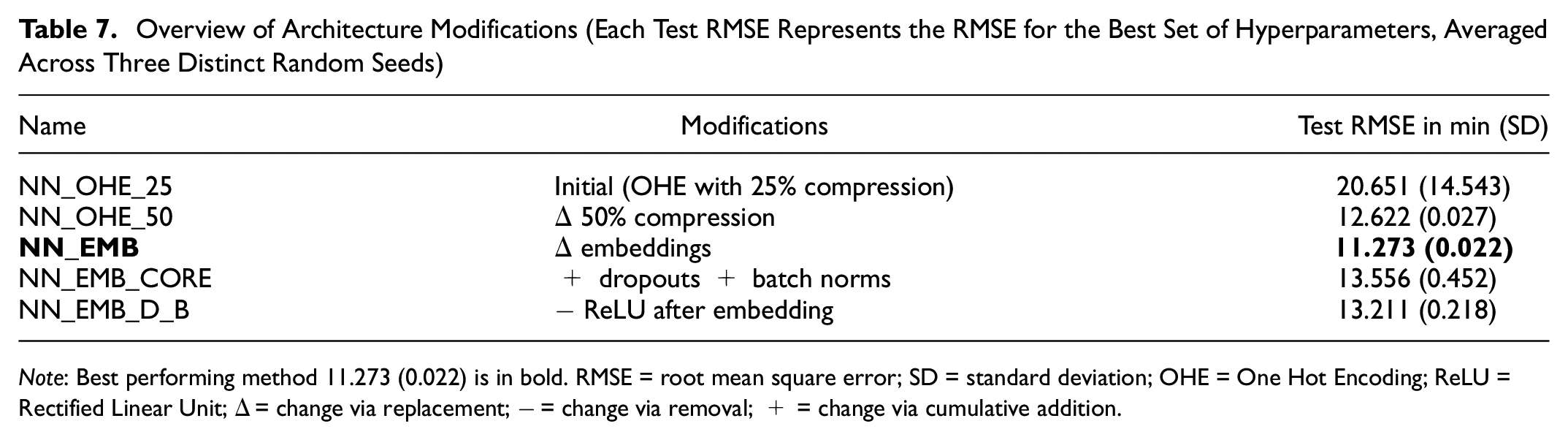
Note: Best performing method 11.273 (0.022) is in bold. RMSE = root mean square error; SD = standard deviation; OHE = One Hot Encoding; ReLU = Rectified Linear Unit; $\mathrm{\Delta }$ = change via replacement; − = change via removal; + = change via cumulative addition.

Transitioning from OHE to embeddings marked a significant shift, facilitating NN_EMB_D_B with a more nuanced representation of the data. This led to a marked improvement in performance; specifically, the RMSE was enhanced from 12.622 min in NN_OHE_50 to 11.273 min in NN_EMB, highlighting the efficacy of embeddings in capturing intricate data relationships.

However, when further modifications were introduced to NN_EMB (particularly dropouts and batch norms) to form the NN_EMB_CORE architecture, there was a discernible degradation in performance. This suggests that the additional regularizing layers introduce unnecessary complexities that outweigh their benefits for this two-layer network. Notably, on removing the nonlinearity after the embedding layer, the performance of the NN_EMB_D_B architecture improved compared with NN_EMB_CORE, thereby indicating that, in this case, additional nonlinearity does not help.

Figure 6 compares the test performance across different architectures, where individual points on the graph represent distinct runs for each architecture. NN_EMB stands out with its uniform performance, demonstrating a test RMSE of close to 11 min regardless of batch size and learning rate variations. This indicates that it is a robust architecture that generalizes well across different configurations. On the contrary, NN_OHE_25 reveals a more varied performance spectrum.

Figure 6.

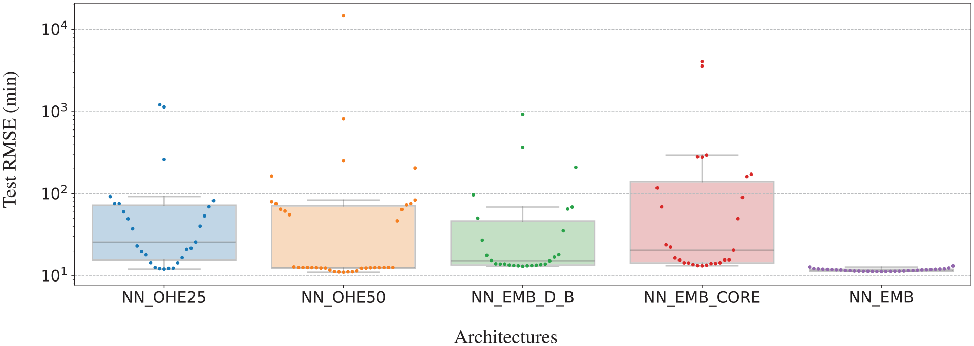
Impact of hyperparameters on the test RMSE. Each point denotes the mean test RMSE for a specific batch size and learning rate combination, averaged over three distinct random seeds. Notably, NN_EMB exhibits consistent performance (an RMSE of approx. 11 min) across various hyperparameter settings.

Figure 7.

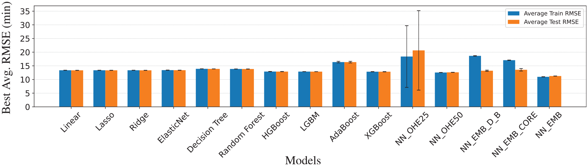
Comparison of the training and test performances of the models.

Meanwhile, NN_EMB_D_B exhibits a notably tighter interquartile range in comparison with NN_OHE_25, NN_OHE_50, and NN_EMB_CORE. This suggests that NN_EMB_D_B offers more consistent performance, with less sensitivity to hyperparameter fluctuations. In contrast, NN_OHE_50 displays a pronounced clustering of data points around its first quartile, indicating inclinations toward a specific performance range. Among all the architectures, NN_EMB stands out not only for its superior performance but also for its remarkable consistency. The data points for this architecture are notably clustered along a line representing the lowest RMSE, indicating that it consistently achieves this performance regardless of minor variations.

Learned Embeddings

In the implemented neural network architectures, NN_EMB_D_B, NN_EMB_CORE, and NN_EMB leverage embedding layers to process categorical variables. As the neural network is trained for block time prediction, these embeddings emerge as rich, multidimensional representations that capture intricate correlations within our dataset. For our visualization, we specifically utilize the embeddings from the best-performing run, notably from NN_EMB. To transform these embeddings into a more interpretable two-dimensional space, we employ t-distributed stochastic neighbor embedding (t-SNE) ( 44 ). Essentially, t-SNE gauges similarities between points in the high-dimensional space and maps them into a lower-dimensional space, ensuring similar data points cluster together. This nonlinear projection technique unveils patterns or clusters that might remain hidden in the original high-dimensional space. Utilizing this technique on our airline embeddings, we obtain a 2-D representation of airlines, as depicted in Figure 8a, which is annotated with IATA labels. We observed that American Airlines (AA), Southwest Airlines (WN), and JetBlue Airways (B6) form a close-knit cluster, revealing shared operational characteristics among them.

Figure 8.

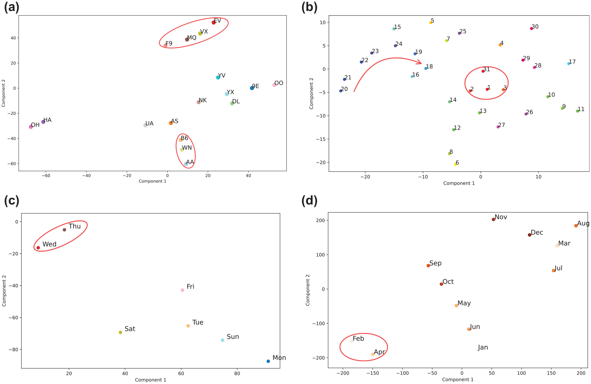
Embeddings from the best-performing NN_EMB run. Red-highlighted clusters and arrows indicate consistent patterns and sequential trends, respectively, across varying learning rates and perplexity values. (a) Airline, (b) DayofMonth, (c) DayofWeek, and (d) Month.

Additionally, the entities F9, MQ, YX, and EV form a separate group, which is distinctly highlighted in red in the figure. Further, we observed that American Airlines (AA), Southwest Airlines (WN), and JetBlue Airways (B6) form a close-knit cluster. Similarly, the entities Frontier Airlines (F9), American Eagle Airlines (MQ), Mesa Airlines (YX), and ExpressJet Airlines (EV) also form a cluster. Both these clusters are distinctly highlighted in red in the figure, indicative of analogous operational attributes amongst their respective members.

The embeddings for the days of the month, as seen in Figure 8b, reveal distinct cyclical patterns. The days 31, 1, 2, and 3 are closely clustered, with a clear sequential trend observed from days 20 to 24. These patterns are consistent across various t-SNE configurations, highlighting the cyclical nature of block time predictions throughout the month. Thursdays and Wednesdays, as shown in Figure 8c, cluster together across different perplexity values and learning rates, while the other days are spread out, demonstrating a significant deviation from this cluster. February and April cluster together in the month embeddings, as showcased in Figure 8d, suggesting similar flight patterns or operational behaviors during these months. However, there might be seasonal travel demands, holidays, or airline promotional activities that dictate the pattern visible, and one would need to delve deeper into external factors to derive concrete insights.

Sensitivity Analysis

We also carried out a sensitivity analysis for the proposed model NN_EMB, as detailed below.

• Error distribution across airlines. Using the computed absolute errors in predictions on the test set across different airlines, it became evident that certain airlines, such as Hawaiian Airlines (HA), Southwest Airlines (WN), and Delta Airlines (DL), had relatively low absolute errors. This suggests that the NN _EMB model was especially proficient at making predictions for these airlines. The distribution of the errors for each airline is shown in Figure 9.

• Error distribution with temporal features. No specific patterns could be discerned from the analysis of errors across months. As seen in Figure 10, the distributions of errors are almost identical; a similar observation was found for DayofWeek. This shows that NN_EMB’s consistency in performance is unaffected by days or months.

Figure 9.

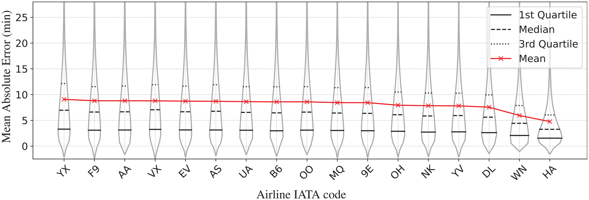
Prediction error across airlines.

Figure 10.

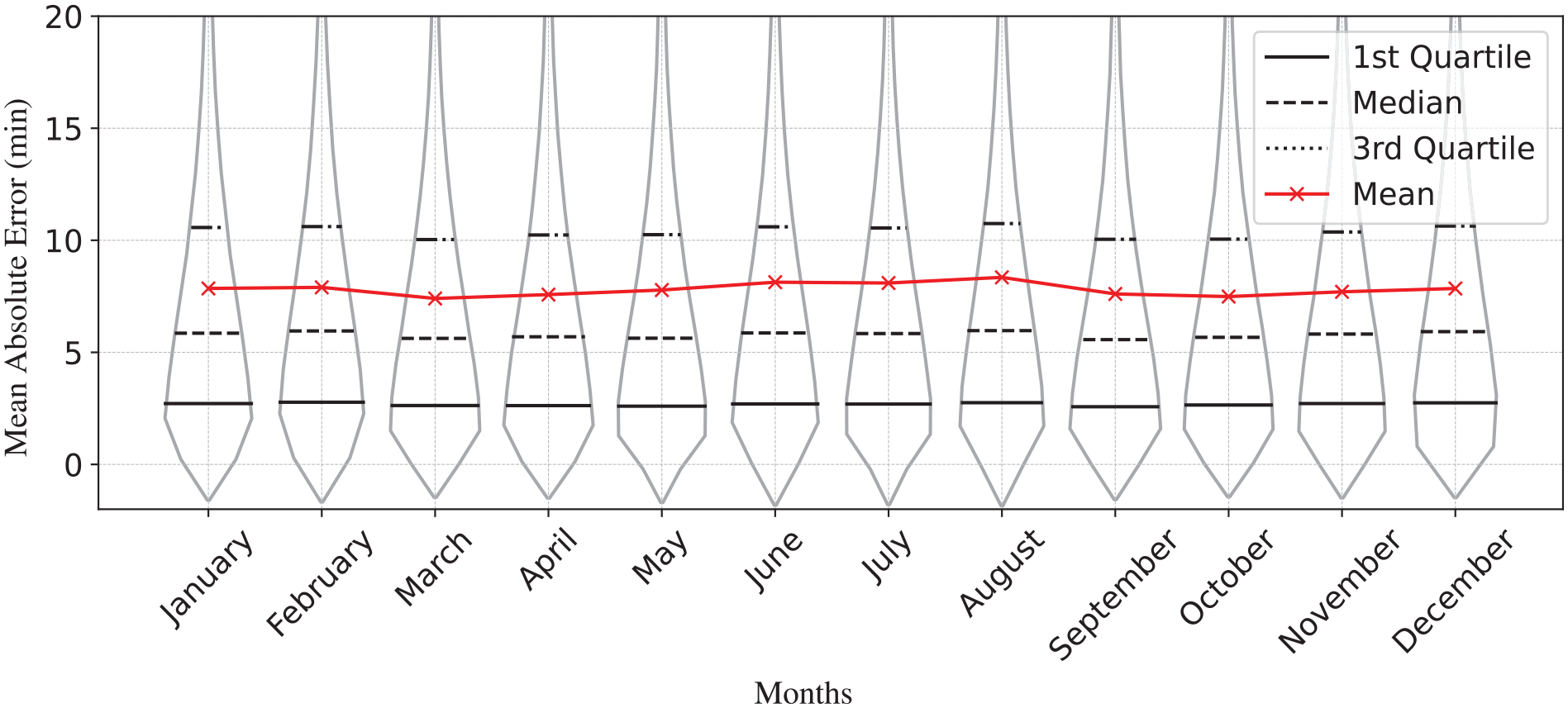
Prediction error across months.

Conclusion

Airline operations, by their very nature, operate under several uncertainties spanning various flight phases. For long-term planning, tasks such as predicting delays, determining block time, and assessing taxi-in and taxi-out durations, among others, take center stage for improving operational efficiencies. To this end, we focused on devising a predictive model tailored to address these challenges for a large-scale dataset (a first, to the best of our knowledge). Our exploration led us to the core insight: traditional encoding methods often fall short when handling the interdependencies and high cardinality of categorical variables. This prompted us to rigorously investigate the role of embeddings in improving forecasting capabilities. Among the neural network architectures explored, an embedding-based neural network architecture (NN_EMB) demonstrated superior performance and consistency properties. In conclusion, our findings emphasize the role of embedding-based representation learning in predictive modeling, especially to capture the complex relationship in high-cardinality features. Future work incorporating additional airline operation priors (aircraft type/age) and diverse data sources remains an exciting possibility to further improve model robustness.