
Abstract
This research provides a methodology for estimating the total societal benefit generated from substituting private vehicle trips with public transportation trips. The external costs of private and public transportation were estimated using a base case travel demand model and then a mode shift was simulated to calculate the effects of shifting one full transit unit (e.g., bus) of demand from a private to public mode. This shift was performed for all origin–destination (O-D) pairs in a region to find the O-D pairs that resulted in the greatest net benefit. These benefits were then normalized using the total automobile vehicle kilometers traveled removed from the network to generate a “transit benefit index.” This methodology was applied to a case study of the city of Bogotá, Colombia. A total of 102 scenarios were simulated: a 2 in base case, and 10 total sensitivity analyses, each including two transit provision alternatives. The results were contrasted with the cost of a new transit unit—a new bus in this case—revealing that the total economic benefit derived from 1 year of increased transit ridership was larger than the financial cost of a new bus to the transit operator. These results suggest that the City of Bogotá should consider further subsidies to transit fares to increase ridership and mitigate externalities.
In 2020, estimates suggest that Bogotá drivers lost approximately 133 h to congestion ( 1 ). Bogotá is known to have one of the best bus rapid transit (BRT) systems globally, however infrastructure quality and status have been declining because of poor land use planning, traffic congestion, and insufficient funding ( 2 , 3 ). Other externalities caused by driving, such as accidents and air pollution, create costs that must be paid directly or indirectly by members of society ( 4 ).
Existing studies often approach mitigating the externalities from driving through pricing (e.g., tolls, HOT lanes, mobility permits) or modal shifts (e.g., transit planning, walking, cycling). The use of tolls to mitigate externalities results in approaches that do not mitigate all externalities equitably ( 5 ). When considering new public transportation routes, transit planning typically accounts for reductions in travel time and prioritizes locations where expected ridership is likely to be greatest ( 6 ), overlooking other external (nonmonetary) costs, which can simultaneously be mitigated by proper transit planning.
This research aimed to develop a method for determining the “critical origin–destination (O-D) pairs” that generate the greatest potential to reduce the marginal external cost on society by increasing the share of those trips made by transit ( 7 , 8 ). Essentially, this research has provided a “transit benefit index” (TBI) that quantifies the benefits of trip switching from private to public modes based on a comprehensive summation of the external costs avoided. Using this index, O-D pairs with varying demands can be directly compared such that those with the greatest benefit per vehicle kilometer traveled (VKT) can be prioritized for transit improvements or transit incentivization through additional routes connecting those O-D pairs or via increased frequency of existing services. Therefore, rather than using travel demand as the sole criterion for additional service above base levels (which would provide the greatest financial return to the transit operator), the proposed method considered the total economic benefit (i.e., which would provide the greatest net benefit to society as a whole).
The remainder of the paper is structured as follows. The next section provides a literature review of external costs of transportation and their estimation procedures. The literature discussed is then synthesized to create a methodology of calculating the externalities of interest, after which all the externalities are monetized. The methodology is then applied to a case study of Bogotá. Finally, the results are discussed, and practical recommendations are deduced before considering the next steps for future research.
Literature Review
External Costs of Transportation
External costs are more difficult to quantify than direct costs but have tangible effects on users and nonusers of the transportation network. These include vehicle emissions, crashes, congestion, and noise-related damage. Previous studies have analyzed the life cycle assessments of different commuter options ( 9 – 11 ), discussing the emissions of different modes of transportation based on passenger miles traveled. Over its lifetime, a bus operating during peak hours produces the least emissions per passenger mile traveled compared with all other motorized transportation modes ( 10 ).
One of the most significant known externalities of driving is congestion, the delay caused by adding additional vehicles to a network. This delay can cause appreciable costs as users lose time on their routes resulting from high volumes of traffic. Congestion costs have been explained using economic models and value of time based on salaries ( 11 ). It is estimated that the United States lost the equivalent of $1,374 per driver in 2019 from congestion ( 1 ), and in 2014, the national congestion cost reached $160 billion ( 12 ).
Ozbay et al. estimated the full marginal cost (FMC) of highway passenger transportation in New Jersey, where one additional unit of demand was simulated between an origin and destination ( 17 ). The marginal costs considered in this study included vehicle operation, congestion, accident costs, air pollution, noise, and maintenance. The results showed that congestion is the dominant externality of transportation in New Jersey and that FMC increases as the percentage of routes that use highways, or higher order links, decreases.
The ASSIST-ME tool is an ArcGIS tool that can be used in conjunction with existing travel demand models created in TransCAD or CUBE to estimate the impacts of proposed policies or transportation plans ( 13 ). A limitation of the ASSIST-ME tool is that it does not perform revised traffic assignments, but instead estimates the shortest path or paths and corresponding travel times between O-D pairs based on the initial traffic assignment provided.
Finally, one study developed a comprehensive transit-based job accessibility index that accounts for the number of feasible alternatives and their frequency in addition to in-vehicle and out-of-vehicle travel times as an example of a “transit critical index.” Transit is less commonly found in the literature studying criticality, robustness, resiliency, and so forth ( 6 , 14–16).
Transit Planning
The priorities of transit planners and governing bodies when it comes to public transportation provision are embodied in the well-studied transit network design problem (TNDP). The TNDP defines the lines, layouts, and operational characteristics to minimize the weighted sum of operator and user costs ( 6 ). External costs and wider economic benefits are excluded from these idealized problem formulations. However, as Newman and Kenworthy suggest in their concept of “transit leverage,” substituting an auto trip with a transit trip has great benefits for the transportation network as a whole beyond operator and user costs (18).
Other studies have focused on the positive impacts of transit developments, in particular the effect that the development of transit options has on road crashes. The operation of BRT can result in reduced crash rates, as shown with the TransMilenio in Bogotá, Colombia ( 14 ). The annual aggregate benefit of decreasing traffic fatalities was $1,776,608 ($5,827,594,881 Colombian pesos [COP]) in 2011. With injury costs, BRT operation provided a benefit of COP$13,732,882,320 (∼US$4,186,624) per year between 2010 and 2013. This example demonstrates the far-reaching benefits transit can have on society, which should be considered in transit network planning.
Methods
Transportation externalities can be modeled using travel demand modeling software (e.g., EMME in this research) and other previously developed methods of estimation. The externalities within the scope of this research are vehicle delays, emissions, noise, and crashes. An overview of the methodology can be seen below in Figure 1.
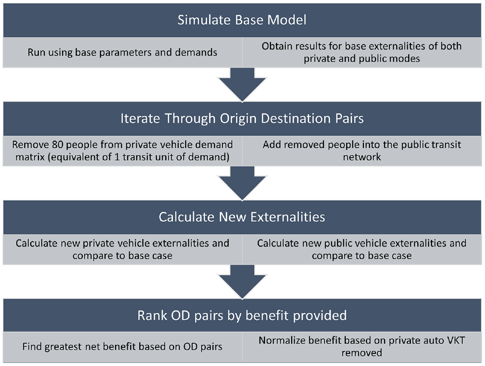
Methodology steps.
Externality Calculations
Total societal cost (TSC) is calculated as an aggregation of total crash costs (TCC), total air pollution costs (TAPC), total noise costs (TNC), and total delay costs (TDC), as shown in Equation 1,

These externalities can be further divided by mode such that TSC can be calculated by private automobile and public transit.
Delay
Delay caused by links over their capacity is multiplied by the number of travelers on the link, resulting in the total vehicle delay for that link, as presented in Equation 2,

where
The delay is then summed across all links to calculate a total delay level for the network shown in Equation 3,

where
TDC is the congestion cost ($),
Value of time (VOT) is in units of $/h ($/h), which is typically taken as half the hourly wage in a given study area but can be slightly less than half ( 11 , 17 ).
Emissions
Emissions can vary greatly depending on vehicle and environmental conditions ( 4 ). Emissions factors (EFs) are applied to the appropriate vehicle subclasses depending on their fuel type, engine class, and age. The effects of changing speeds are not captured in detail within these EFs; however, assumptions are made based on the link type. Factors for arterial roads are developed using a ratio of highway to arterial emissions and applied to EFs based on the link type ( 19 ). EFs are generally stated in grams per vehicle kilometers traveled (g/VKT) and are thus applied to the traveled distance of the vehicles of interest as shown in Equation 4,

where
j is the link identifier for links of the highway or arterial regime,
di is the vehicle kilometers traveled of vehicle type i (km), and
EFkij is the associated emissions factor of vehicle type i and pollutant k (g/km) on road type j ( 19 – 21 ).
The arterial factor for bus emissions is not applied as it is assumed that the impact of the link type will be negligible given that buses are required to stop frequently for passengers. The emissions of each vehicle type are summed to find the overall emissions of each pollutant and multiplied by the value of that pollutant, as seen in Equation 5,

where
Noise
The use of hedonic housing prices has been the focus and method of estimation of noise damage in several papers in the past (
11
,
6
,
17
). As house prices are subject to several other external factors, this research focuses on the measurable impacts of noise on individuals (
22
). Traffic noise estimation can be done using the RLS 90 method, which is commonly used to calculate traffic noise generation (
23
–
25
). It considers vehicle speed, velocity, and percentage of heavy vehicles (
26
). In dense cities, mixed land use between residential and office buildings results in people staying within city and downtown limits throughout the day and being affected by noise both on- and off peak. Noise values are calculated per link at a base distance of 25 m, assuming all vehicles are traveling at 100 km/h (
26
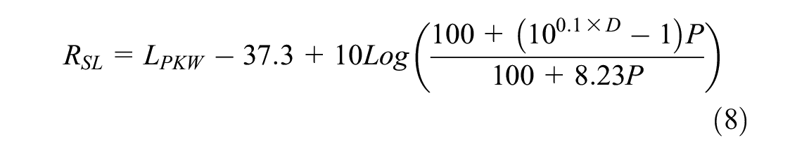
). The value calculated is an

where Q is the hourly volume on a link, and P is the heavy vehicle percentage. The final generated noise ,
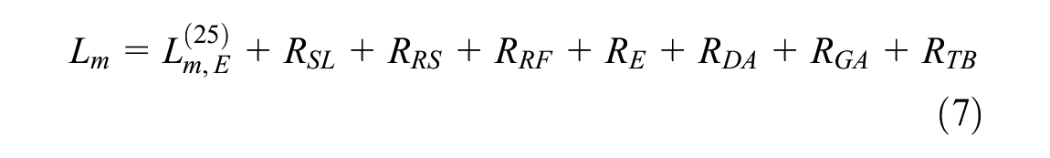
where
All correction factors have units of decibels (dB).
Owing to a lack of topological data, it is assumed that the road surface has a negligible impact and that roads are within the 5% standard gradient.
where


where
D = difference between the mean noise of light vehicles and heavy vehicles (dB).
An average sound level for each zone (N) is estimated using each link (i) in the zone. Given that a zone is sufficiently dense, it is assumed that the population density is uniform such that an average person/m2 value is given to the zone. Assuming that noise levels beyond the 25-m point are below the background noise level, the area of impact from the noise generated by vehicles can be calculated if the number of lanes and the lane widths are known. The equation for estimation of the area impacted by the average noise produced by link i in a zone N is given in Equation 12,
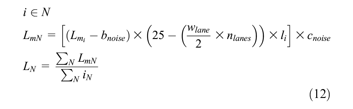
where
The monetary cost of noise levels is then applied to the average noise level in the zone and the population density assuming a uniform distribution of people across the zone. This is shown in Equation 13,

where
TNC = total cost of noise ($),
Crashes
To evaluate crash externalities, value of statistical life (VSL) is typically used for fatalities. VSL can be determined though willingness-to-pay (WTP) surveys for reductions in risk in transportation. A meta-analysis of these types of surveys was undertaken in which over 850 estimates of sample mean adult VSLs from 38 countries were analyzed ( 28 ). The mean traffic VSL among those estimates is US$6,861,777 with a standard deviation of $820,807 (2005 U.S. dollars). The range of values is also extremely large with the minimum value being US$21,086 and a maximum value of US$112,000,000.
For crash rates, the most common explanatory variables are VKT and vehicle flow rate, however models can be made more accurate with additional explanatory variables ( 29 , 30 ). Owing to this model’s scale, the only factors considered for this analysis are the base VKT per road type and the base number of crashes as shown in Equation 14,

where
r is the estimated peak hour–mode, m, crash rate (crash/VKT) for injury type, i, on road type, j; and
d is the base VKT of mode, m, on roadway type, j.
Given a change in the VKT of a mode on a given road type, a proportional change in crashes would be expected based on Equation 15,

where

where
Transit
Transit assignment and analysis utilized two methods. The first method (Method #1) edits the transit demand within a Python script and the resulting matrix is input into EMME to run the simulation. Transit users are assigned based on an optimal strategy, in which users consider waiting and transfer times when determining the best route to reach their destination ( 31 ). For any lines over capacity, the script adds enough hypothetical vehicles to the line to meet the line demand, and calculates new externalities based on the additional vehicles.
The second method (Method #2) does not rely on performing the extended transit assignment for every iteration. Instead, the “shortest path” tool in EMME is used to find the set of links that represent the shortest path between any O-D nodes. After removing the auto demand from a particular O-D pair, the length of the shortest path is calculated, and externalities are then recalculated using a hypothetical “average transit unit” set on the shortest path.
Transit Benefit Index
The externalities saved are normalized based on VKT removed from the network to find a value of savings per VKT removed—the TBI —and has units of $/VKT removed, which is given by Equation 17,

where
Data
This methodology was applied to a case study of Bogotá, Colombia. Bogotá has many open data sources and publishes transportation metrics and findings on the SIMUR open database (Sistema Integrado de Información sobre Movilidad Urbana Regional), or on the Colombian government website (datos.gov.co). The Department of Transportation of Bogotá (Secretaria Distrital de Movilidad) provided their latest EMME travel demand model for this study. This includes a calibrated 2019 model, which was created using their most recent household travel survey and includes data on private auto, public transit, taxi, and pedestrian trips. This data allow for the most accurate estimation of trip changes and the effects that they have on total externalities.
In 2017, public transportation made up 35.8% of all trips made in Bogotá. The full breakdown of Bogotá’s mode split can be seen in Figure 2. Pedestrian travel also made up approximately 24% of trips, which implies that residents can complete sections or full trips within existing pedestrian infrastructure and demonstrates the feasibility of switching between private and public modes.
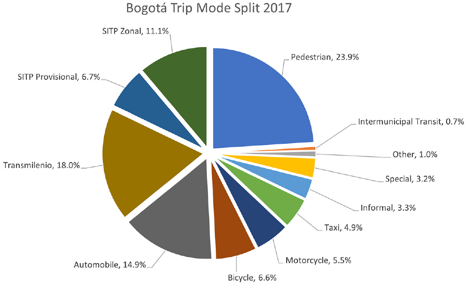
Trip mode distribution in Bogotá ( 32 ).
An EF database for Bogotá was recreated using local information of activity rates, speed profiles, vehicle population distribution and age, meteorological effects, and fuel composition after it was noted that EFs from before 2010 may not reflect the reduction in sulfur content in diesel as effectively as the renovation and deterioration of passenger vehicles ( 33 ). The final EFs obtained from the MOVES-2014a model and comparison with the existing local EFs for gasoline and diesel vehicles can be seen in research undertaken by Ramirez-Gamboa et al. ( 33 ). The emissions costs are developed based on the European handbook and are shown in Table 1, which uses local EFs ( 27 , 33 ).
Base Emissions Rates and Costs for Private Vehicles
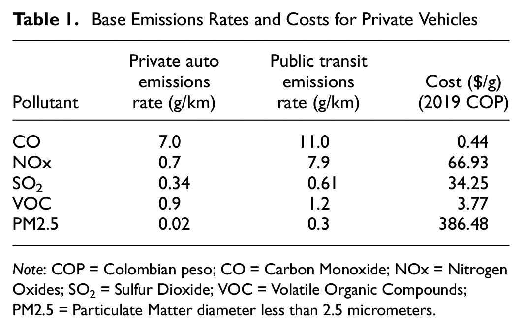
Note
Through the SIMUR open data portal, crash data from 2015 to 2020 titled “Anuario de Siniestralidad vial de Bogotá” (Yearly Traffic Crash Report of Bogotá) includes a breakdown of the crashes by mode, road user victim, and severity for private and public transportation modes. Annual road fatalities can be seen in Figure 3, whereas road injuries can be seen in Figure 4.
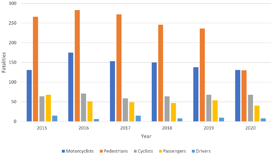
Fatalities by mode from 2015 to 2020 ( 34 ).
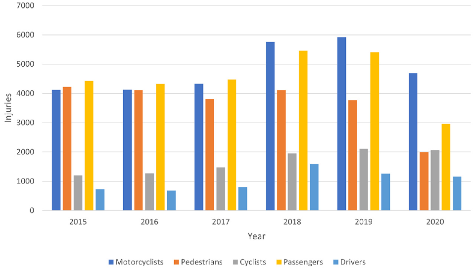
Injuries by mode from 2015 to 2020 ( 34 ).
The crash data were further divided into “highway” and “nonhighway” crashes based on the raw data provided in the SIMUR database and summaries of these crashes can be seen in Figure 5. Since existing data were not available for the total VKT, it was assumed that the estimated VKT obtained from Bogotá’s EMME model was representative of the total VKT for the purpose of estimating crash rates. Victims of fatalities and injuries were further divided into frequency depending on the time of day. The majority of crashes are caused by the modes that are being investigated in this paper, namely, private light vehicle transportation and public transportation ( 34 ).
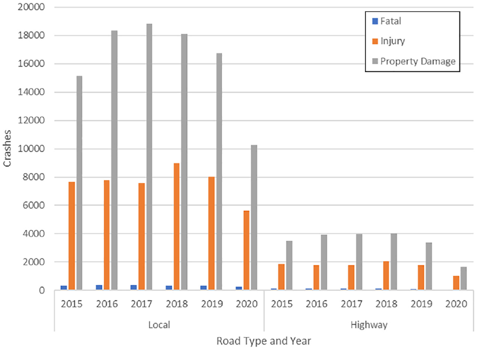
Highway and local crashes in Bogotá per year (2015 to 2020).
Although there were fewer fatalities overall, a greater share of them occurred on highways, as expected, owing to the higher speeds that are experienced on highways. However, for both fatalities and injuries, less than 30% of averaged crashes occurred on highways. Were trips removed from local roads, they would be expected to have a greater impact on the overall crash externality.
A local study of VSL in Bogotá for transit related fatalities was calculated to be approximately COP$128 million (∼US$39,022) ( 35 ). This value was derived for the “analysis of the impact of crashes” and based on a stated preference survey using a binary probit model to estimate WTP for the reduction of risk of fatal crashes in the context of public transport in Bogotá. The value obtained is approximately 22% of the international average values with other countries’ VSLs ranging between COP$560 and 590 million (∼US$170,700 to 180,000) ( 34 ).
Costs associated with hospital visits after a logged crash report in Bucaramanga, Colombia were found to quantify injury costs from 2018 to 2021. Bucaramanga has the highest gross domestic product per capita of any city in Colombia and data are taken to be representative of hospital costs in other large cities in the country. The data contained 15,111 relevant entries, which included crashes involving bus, auto, and motorcycle modes. The average car and bus injury cost was COP$757,162.51 and $317,264.34 with a standard deviation of $1,899,401.17 and $601,265.14, respectively.
Since no existing studies were found for estimating costs caused by excessive noise in Bogotá, the European standard values were used. Noise costs were estimated using a range of costs depending on the decibel level over the threshold.
Results
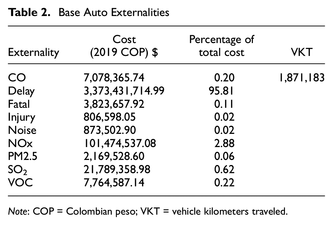
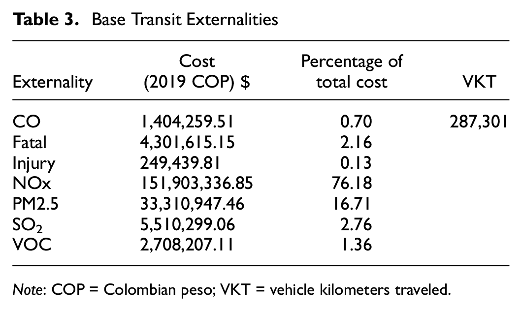
The required simulations were performed using Bogotá’s travel demand model in EMME, comprising the base network, private and public demand matrices, and link cost functions. Bogotá’s annual crash report showed the base number of fatalities between 8 and 10 a.m. for auto and transit were eight and nine, respectively, and 298 and 135 for injuries ( 34 ). These numbers were divided by 365 to estimate daily fatalities and injuries. After running the base simulation, the total costs obtained from the traffic model can be seen in Tables 2 and 3.
Base Auto Externalities
Note
Base Transit Externalities
Note
Although private travel generally has high emissions and externalities, public transit resulted in higher PM2.5, NOx, and fatality costs despite having only 15% of the total VKT of private auto. The emissions results are likely to be the result of the differences in efficiencies of gasoline-powered cars and diesel-powered buses. For fatalities, although Bogotá has a high-class BRT system in place, there were more fatal crashes involving buses during the AM peak hour than private vehicles. These fatalities typically involve crashes between motorcycles or private vehicles with buses that are not integrated into the BRT system. Conversely, private vehicles were involved in over twice as many crashes resulting in only injuries, which tend to have higher costs than transit injuries.
The share of the various externalities can be compared with the ASSIST-ME model ( 13 ). The externalities are grouped into the general categories, noise, congestion, air pollution, and crashes. For the Bogotá case study, private auto and public transit externalities were summed when finding the share of externalities. The comparison resulted in a very similar share of externalities with the largest difference being crash costs for which the ASSIST-ME model states that crashes make up 7% of externalities whereas the Bogotá case study resulted in less than 1%. This discrepancy was expected as the VSL used in the Bogotá case study was on average 22% lower than international averages.
A total of 49 O-D pairs within the origins of interest had a demand of at least 80 people (i.e., equivalent to 1 transit unit—a bus in this case), and were analyzed. The selected O-D pairs can be seen in Figure 6.
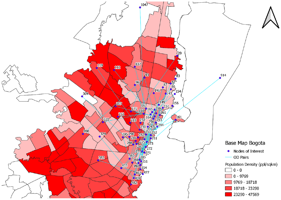
Origin–destination (O-D) pairs of interest in downtown Bogotá.
Figures 7 and 8 below represent the top 10 O-D pairs by TBI per transit provision assignment method. This TBI considers the externalities added by the increased public transit demand.
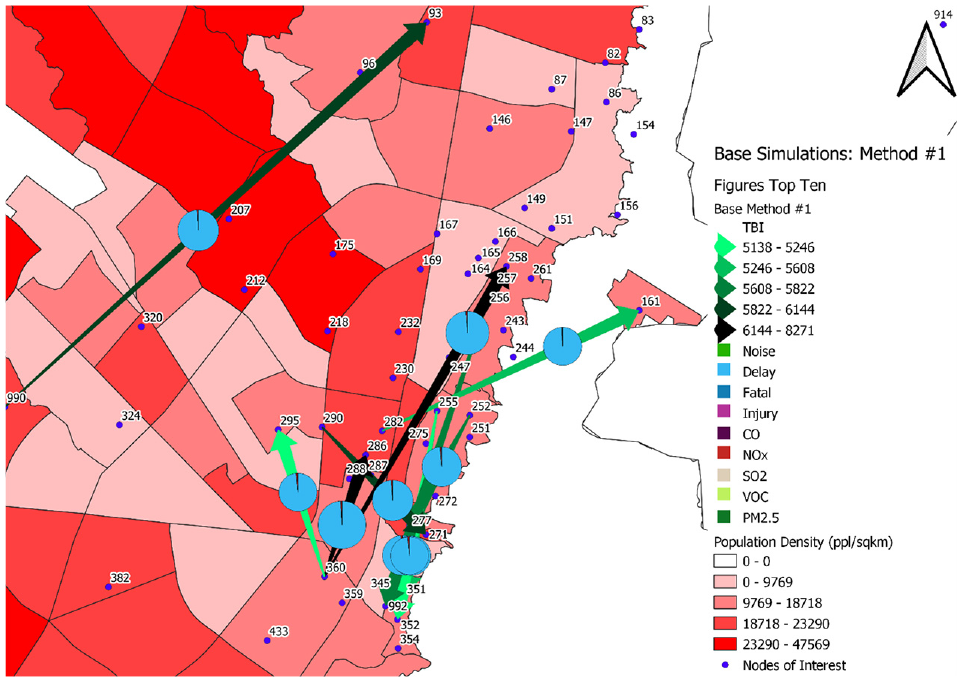
Top 10 origin–destination (O-D) pairs by transit benefit index (TBI) in the base case (Method #1).
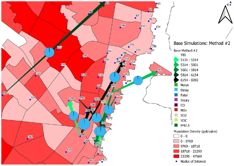
Top 10 origin–destination (O-D) pairs by transit benefit index (TBI) in the base case (Method #2).
Figure 9 contains the breakdown of the externalities saved for the top O-D pair (O: 360, D: 286).
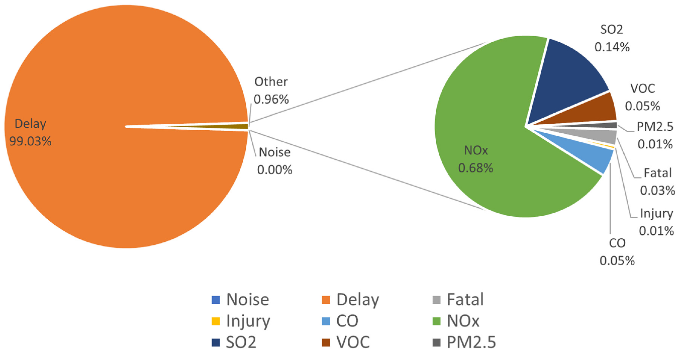
Breakdown of saved externalities in the base case for origin–destination (O-D) 360,286 Method #1.Note: CO = Carbon Monoxide; NOx = Nitrogen Oxides; SO2 = Sulfur Dioxide; VOC = Volatile Organic Compounds; PM2.5 = Particulate Matter diameter less than 2.5 micrometers.
The breakdown showed that delay was the externality that provided 99% of savings in the base case with other externality savings accounting for only 1%. This trend was seen in all O-D pairs in the top 10 list.
Sensitivity Analyses
Five sensitivity analyses were performed, which included changes in emissions rates, assuming electric buses with no emissions, 0% VOT, 100% hourly salary VOT, and a higher VSL case to determine which externalities were robust against changes in valuations of externalities. The results proved robust against almost all sensitivity analyses performed with only the 0% VOT case producing a different top 10 list compared with the base case.
Discussion
In the base case, delay generated 90% of the externalities in the network, emissions accounted for approximately 9%, and crashes accounted for less than 1%. The share of externalities caused by crashes was lower than expected, however it is explained by the VSL used in Bogotá being much lower than values used in either North America or Europe, where most existing literature is found. These proportions of externalities are in line with previous literature that concludes that delay has the greatest share of savings.
Net savings were normalized by the amount of private VKT removed from the network to produce the TBI, which was then used to rank all the O-D pairs analyzed. The TBI presents a straightforward way to compare the savings generated by the O-D pairs and provides decision makers with a thorough method for prioritizing transit plans. The results showed that the top O-D pair represented savings of COP$8,271.35 (US$2.52) per private auto VKT removed and a net sum of COP$2,436,197.95 (US$742.70) in externality savings for the network per AM peak hour. Extrapolated over a year, it would present savings of COP$2,150,550.70/VKT (US$655.62/VKT) per year, and a sum of savings of COP$633,411,468.25 (US$193,102.66 2019) per AM peak per year.
When compared with the ticket price of a “TransMi” (combined transit and metro) ticket using Bogotá’s preloaded card of COP$2,300 (US$ 0.70) per trip, the resulting savings bring in more value than the ticket price per kilometer. If we assume that a full bus results in 80 people purchasing a COP$2,300 ticket, that amounts to $184,000 (US$56.09) in revenue for a one-way transit trip. In the base case, the results showed that the savings in externalities were 13 times greater than the revenue from fares. It could therefore be argued that the benefit of removing private vehicles from roads provides enough savings to fully subsidize ticket prices to encourage more public transit ridership—assuming there is a nonzero demand elasticity to transit fares.
Using the BRT Planning Guide, a 40-ft diesel bus is estimated to cost approximately US$250,000 and a 60-ft articulated diesel bus $500,000 (2019 U.S. dollars) ( 36 ). Considering these costs, just 1 year of the full savings gained from the top O-D pair (of $742.70 per AM peak) is larger than the initial cost of a bus. Recognizing that savings from other modes (e.g., taxis, motorcycles, trucks) are not captured, it can be assumed that this hypothetical payback period would drop further. This value is relevant to this research and its assumptions as it is presumed that a new bus could be added to existing lines to maintain current service levels (therefore, requiring some sort of capture and transfer mechanism of the economic savings to the transit agency).
Key sensitivity analysis outcomes were that the largest externality currently valued was lost time (i.e., delay), as savings in delay comprised over 90% of the savings found in all scenarios in which the value of time was greater than 0, whereas NOx provided the largest savings other than delay. It was also found that in many cases, the noise externality increased as private vehicle traffic was removed since more noise is generated by faster moving vehicles.
Considering air pollutant valuations could change in the future with newer findings about air pollution and climate change, some countries may value reducing air pollution more than other externalities.
Because of the low VSL in Colombia, savings gained through crashes would not be high enough to prioritize removing vehicles from local roads where fatalities are more common. Even when considering a higher VSL, the results did not influence the top 10 list of O-D pairs.
Limitations
As this study concerns itself with a large area and several external factors, several assumptions were made in the formulation of scripts and simulations. These assumptions should not change the findings substantially and attempts were made to mitigate the effects of these limitations.
In a large-scale travel demand model, having an accurate and dynamic EF for vehicles is difficult and EFs were assumed to be static for each mode. In-vehicle travel time for transit users was not considered because detailed transit information was not available. It is expected that transit travel times would be greater than private vehicles, however the removal of vehicles on corridors would result in lower travel times for transit users as well. During high congestion events, it is common that speeds fall below the accurate range of the RLS 90 method ( 25 , 26 , 37 ). Other factors such as pavement structure, building absorption, and height of the noise receiver were not accounted for either. It is assumed that the noise level calculated would be a “worst case scenario” in which no buildings or structures mitigate noise on the roadsides and a constant noise level is experienced. This study only considered vehicle kilometers traveled on various link types for crash rates. The methodology did not take into account the interaction between different crash rates. The VSL chosen for Bogotá came from a local study, however, this is subject to change as the socioeconomic situation in Colombia and Bogotá may change ( 35 ).
Transit assignment assumptions are highly idealized and may not always represent real world capabilities. Method #1, which adds travelers to existing transit services, is possible in the downtown core of Bogotá where the transit network is dense. The externalities of the Bogotá metro were outside the scope of this study and no metro transit units were added in either of the methods presented. This study also did not consider the detailed financial costs of adding a transit unit to the network, which includes the purchase price of the vehicle and any labor that would be required to operate and maintain it. In Method #2, in which a new theoretical transit line was added, the infrastructure costs of adding additional transit stops were not considered.
Finally, the externalities modeled in this study were only for private light vehicles and public transit buses. Since delay savings to other modes were not included, all numbers presented were a conservative estimate of the total savings expected from the substitution of private vehicles to public transit.
Conclusions
This study proposed and demonstrated a comprehensive way of determining the savings gained from the removal of private vehicle traffic on a transportation network, while providing a novel index to rank and prioritize areas for transit provision or improvement. The method is easy to modify and could be applicable internationally given the required data and could be altered easily to reflect the priorities of a given region.
A case study was performed for Bogotá, Colombia using a local travel demand model. Key findings showed that the benefits of public transportation projects and ridership were not being properly reflected in current policy decisions. The case study in Bogotá showed that replacing private vehicle traffic with public transportation resulted in a greater economic benefit than current ticket fares. The benefits could also be leveraged in the cost–benefit analysis of the purchase of new transit units to service existing or new routes.
In future studies, this method could be improved through the use of dynamic EFs that further account for speed and stop-and-go traffic, more accurate noise modeling, and local cost factors for emissions. For greater accuracy, this methodology could also be implemented with a microsimulation model to capture the details of delay and emissions, as well as passenger wait times at transit stops. Additionally, the proposed methodology could be extended to identify certain O-D pairs for which insufficiently effective (i.e., indirect) transit service is currently provided, and for which there may be both a market case (overall travel demand) and social case (disproportionately large decrease in negative externalities) for adding a new route to better serve that O-D market.
Finally, a detailed examination of fares, transit costs, and the financial viability (including potential government transfer mechanisms) would complement the detailed examination of benefits provided by the current framework.
Footnotes
Acknowledgements
The authors thank the City of Bogotá for providing the travel demand model for analysis.
Author Contributions
The authors confirm contribution to the paper as follows: study conception and design: R. Rendel, C. Bachmann; data collection: R. Rendel; analysis and interpretation of results: R. Rendel, C. Bachmann; draft manuscript preparation: R. Rendel. C. Bachmann. All authors reviewed the results and approved the final version of the manuscript.
Declaration of Conflicting Interests
The authors declared no potential conflicts of interest with respect to the research, authorship, and/or publication of this article.
Funding
The authors received no financial support for the research, authorship, and/or publication of this article.