Sage Journals: Discover world-class research

Abstract

Methods for identifying optimal decisions for dedicated bus lane locations (DBLs) on a network have been extensively studied in the literature. However, the impacts in relation to changes to car and bus delays of deploying a DBL on a given link largely depend on where other DBLs exist on the network. Therefore, for a network-wide location optimization or a bus lane design problem, linkages exist between decision variables. Typically used metaheuristic methods to optimize DBL locations, such as genetic algorithms (GAs), do not perform well for such problems with linkages between decision variables. To this end, this paper has two novel contributions to the literature by (a) demonstrating that the linkage problem exists, and (b) testing different heuristic algorithms that are more suitable than GAs for optimizing the locations of DBL on a network. The linkage problem in the location optimization of DBLs is demonstrated by enumerating all possible bus lane locations in a small grid network. Next, optimization algorithms that do not enumerate all possible bus lane locations that are capable of learning linkages between decision variables, namely Bayesian algorithm and a population-based incremental learning algorithm, are proposed. These algorithms are compared with two types of GAs in relation to consistency and quality of the solutions, and exploration capability. Results show that algorithms that can learn linkages between decision variables perform better than the GAs.

Keywords

bus lane bus transit systems optimization planning and analysis public transportation transportation network modeling

Transportation planning and management involve countless decisions that can have effects that span the entire network. Because of the importance of these decisions, many researchers have studied methods that can identify the optimum decisions for a given problem on a network such as traffic signal coordination ( 1 , 2 ), traffic signal timing ( 3 , 4 ), toll pricing ( 5 – 8 ), bus fare ( 9 ), network design ( 10 , 11 ), transit network design ( 12 , 13 ), and bus lane placement ( 14 – 23 ). Specifically, the dedicated bus lane (DBL) implementation location selection problem has been formulated as a combinatorial optimization problem in the literature ( 14 – 22 ). Typically, a bi-level methodology is used. The upper level of these methods determines the optimal combination of bus lane locations to minimize total travel time, while the lower level evaluates the network to determine the travel times. The upper level of these models is solved using Benders’ decomposition ( 21 ), branch and bound ( 19 ), or genetic algorithm (GA) (14 –18, 20), whereas the lower level is typically solved with the Akcelik or Bureau of Public Roads cost functions. The use of metaheuristic algorithms at the upper level can often find reasonably good solutions that can be used for planning and decision-making purposes. However, for the problems that involve optimization of capacity-changing network modifications (e.g., bus lane placement), basic evolutionary algorithms are not ideal choices for optimization because of the linkage problem between decision variables.

In the literature on metaheuristic algorithms, the linkage between decision variables is defined as the influence of one variable on another variable. From the transportation optimization perspective, linkage means that the effect of one network modification decision depends on the existence of another network modification. For example, any modification of signal settings at an intersection can also affect the delay in neighboring intersections. Thus, for an optimization problem considering signal settings in an area, the decision variables are dependent on each other. This dependence makes it more difficult for basic evolutionary algorithms, especially GAs, to efficiently find the optimal solution, as GAs do not explicitly account for the dependency in the decision variables. Previous studies have found that unaccounted linkages between decision variables can significantly impact the performance of GAs ( 24 , 25 ).

The issues caused by linkage can be avoided by significantly increasing the exploration capability of GAs using several modifications such as diversity control measures, increasing the size of the population, and adopting an aggressive mutation approach. However, as these methods increase the computation time of the optimization algorithm, these methods may not be viable for optimization problems that are computationally expensive to evaluate, for example, microsimulation. Several methods can be used to make GAs capable of learning linkages. These methods include mutation (e.g., inversion) ( 26 ), crossover regulating non-coding bits (e.g., metabits and punctuation marks) ( 27 , 28 ), and crossover methods (e.g., Masked crossover, shuffle crossover, adaptive uniform crossover, selective crossover, linkage evolving genetic operator) ( 29 – 33 ). These are simple methods as they only utilize the fitness of each solution to learn linkages between decision variables. Some more advanced crossover methods use probabilistic models for the crossover operator, such as general linkage crossover ( 34 ), adaptive linkage crossover ( 34 ), and linkless self-distancing GA ( 35 ). Regardless, if a high number of linkages is present in the optimization problem, these methods are not effective in identifying and learning the linkages. For such problems, an optimization method capable of learning the dependencies between the decision variables is needed.

Messy GAs and estimation of distribution algorithms are the two main types of evolutionary algorithms capable of learning linkages. The main difference between these two types of algorithms is how the existing linkages between the variables are identified. Messy GAs first conduct a partial enumeration of the solution space to select promising building blocks to identify linkages, and then use these building blocks to continue with a solution method similar to the basic GA. Some common examples of messy GAs are messy GA, gene expression messy GA, fast messy GA, ordering messy GA, and structured messy GA ( 36 – 39 ). The need for partial enumeration makes these types of algorithms infeasible to use for simulation-based transportation optimization problems because of the required computation time. On the other hand, estimation of distribution algorithms identify the existing linkages within the decision variables by leveraging probability theory. Some of the commonly used estimation of distribution algorithms include population-based incremental learning (PBIL), extended compact GA, bivariate marginal distribution algorithm, factorized distribution algorithm, edge histogram-based sampling algorithm, and Bayesian optimization algorithm (BOA) ( 40 – 45 ). These methods construct and sample probabilistic models of linkages, and do not require a computationally expensive partial enumeration.

To the authors’ knowledge, no existing work has shown the problem with dependency in location selection problems in the transportation context and explored potential heuristic solutions that can deliver an improved performance in light of this dependency. To this end, the first goal of this paper is to illustrate the linkage problem among the location of DBLs on transportation networks. More specifically, this study will demonstrate how implementing a DBL on a given link can change the benefits or disbenefits of implementing a DBL on a different link. DBL locations are the ideal subjects for this study because of the trade-off between reduction in transit delay and reduction in capacity of non-transit traffic. To do so, a bi-level algorithm will be formulated and enumeration will be used at the upper level to evaluate changes in travel time considering all possible combinations of DBL locations on a small network. The second goal of this paper is to evaluate optimization algorithms (without enumeration) that can account for linkages in the data, that is, more specifically the dependency among the locations of DBL implementations, to find near-optimum solutions. This paper will explore the use of estimation of distribution algorithms to optimize transportation infrastructure networks. The PBIL and BOA are chosen as candidates in this paper specifically for their popularity and ease of implementation.

The optimization results of two GAs and two estimation of distribution algorithms will be compared.

The rest of the paper is organized as follows. The next section describes the network evaluation methodology and using this method the dependency problem is demonstrated by enumerating the total travel time of all combinations of locations for possible DBL implementation in a small network. Then, the tested optimization methodologies are described in the Solution Methods section. The test network and experiment setup, along with the results of four different optimization algorithms are presented in the Results section. Finally, some concluding remarks are provided in the last section.

Network Evaluation Methodology

In this study, the bi-level methodology used in Bayrak and Guler ( 20 ) is used to evaluate the network. In this optimization framework, the lower level evaluates a set of implementation locations of DBLs by using link transmission model (LTM) to estimate total travel time of network users. The LTM is chosen as it can account for queue spillbacks caused by congestion and provide more accurate estimations of change in car travel time resulting from the implementation of DBLs. The LTM is a dynamic network loading model that provides an approximate solution to the kinematic wave problem at the network scale ( 46 ). The inputs to the LTM are network parameters (e.g., capacity of links, free-flow speed, etc.), simulation parameters (e.g., time step, simulation duration), and an origin–destination matrix (e.g., number of vehicles wanting to travel between an origin and destination for each time step). The LTM propagates aggregated groups of vehicles along a link and distributes them at nodes (i.e., intersections) at discrete time intervals according to the principles of kinematic wave theory while assuming a triangular fundamental diagram ( 47 , 48 ). Triangular fundamental diagram is a piecewise linear function of flow with respect to density. The main output of the LTM is the cumulative vehicle diagrams at the upstream and downstream end of each link. Other outputs, such as link travel times, flows, and densities, are obtained from the cumulative diagrams by using queuing theory. However, as the LTM is an aggregated model, bus movements are not explicitly modeled. To model transit movements, a separate tracking algorithm is used. The tracking algorithm uses the cumulative vehicle counts of each link to track buses individually. Tracking is done by estimating link entry and exit times of each bus on all links as they travel along their bus route. The bus-tracking algorithm has two underlying assumptions: (1) buses travel at the same speed as cars on links without DBL, and (2) buses travel at free-flow speed on empty links or links with DBL. The bus-tracking algorithm works as follows:

Step 0: Initialize the algorithm when a bus is dispatched.

Step 1: When a bus enters a link, tag the upstream cumulative vehicle number of the link as a bus, $n_{b}$ , and record the current time step, $t$ , as the bus entry time to the link, $t_{entry}$ .

Step 2: Proceed to the next time step, $t$ .

Step 3: Check the exit condition:

• For an empty link, or a link with a dedicated bus lane:

○ The exit condition is met if the signal is green and current travel time of the bus on the link, ( $t - t_{entry}$ ), is greater than the free-flow travel time.

• For a link that is not empty or does not have a dedicated bus lane:

○ The exit condition is met if the downstream cumulative vehicle number of the link is greater than the tagged bus number, $n_{b}$ .

• If the exit condition is met, record the current time step, $t$ , as the exit time, $t_{exit}$ , and proceed to Step 4. Otherwise, return to step 2.

Step 4: Check whether there is a bus stop at the downstream end of the link.

• If there is a bus stop, update the on-board passenger count by performing boarding and alighting operations based on the origin–destination matrix.

• Otherwise, proceed to Step 5.

Step 5: Record the link bus travel time as $t_{exit} - t_{entry}$ , and check the termination criteria.

• If the current link is the last link of the bus route, terminate the algorithm.

• Otherwise, proceed to the next link on the route and return to Step 1.

For simplicity, in this paper it is assumed that the boarding and alighting of passengers at bus stops are instantaneous. Thus, the exit time of the bus from a link does not depend on the number of passengers at the bus stop. However, as the number of boarding passengers and the number of passengers waiting at each bus stop is known at all times, a dwell time model can be easily implemented in the algorithm by adding an exit condition to Step 4 of the algorithm.

Because the LTM propagates vehicles at discrete time steps, implementing a dynamic route and mode choice is possible. In this paper, mode and route choice of network users are updated using logit models. These logit models are based on link travel times of buses calculated from the bus-tracking algorithm and link travel time of cars calculated using cumulative vehicle diagrams. Equations 1 to 3 are used to update the modal split at the end of each signal cycle.

P_{m}^{OD} = \frac{\exp (U_{m}^{OD})}{\sum_{M} \exp (U_{m}^{OD})}

(1)

U_{Car}^{OD} = C_{car} - a_{car} {TT}_{car}^{OD}

(2)

U_{bus}^{OD} = C_{bus} - a_{bus} {TT}_{bus}^{OD}

(3)

where $P_{m}^{OD}$ is the probability of a commuter using mode $m$ from origin $O$ to destination $D$ , ${TT}_{car}^{OD}$ is the travel time by car between origin $O$ and destination $D$ , ${TT}_{bus}^{OD}$ is the travel time by bus between origin $O$ and destination $D$ , $C_{m}$ and $a_{m}$ are the calibration coefficients that represent the mode choice behavior of the network users. The travel time by car, ${TT}_{car}^{OD}$ , is calculated as the sum of the link travel times on the fastest route (the route with shortest travel time) between the origin and destination (OD) pair. The bus travel time, ${TT}_{bus}^{OD}$ , is calculated as the sum of in-vehicle bus travel time (determined as the sum of bus link travel times), the walking time to the bus stop, the waiting time at the bus stop, and the transfer time (at most one transfer is allowed). It is assumed that bus passengers are assumed to use the bus stop closest to their origins and if their journeys require transfers, passengers use the route with the fewest number of transfers.

A similar logit model is also used to update the route choice dynamically. Different from the mode choice, route choice is updated at every time step at every intersection by using travel times from a given intersection to every destination.

P_{r}^{ID} = \frac{\exp (a \times {TT}_{r}^{ID})}{\sum_{R} \exp (a \times {TT}_{r}^{ID})}

(4)

where $P_{r}^{ID}$ is the probability that route $r$ from intersection $I$ to destination $D$ is chosen, ${TT}_{r}^{ID}$ is the travel time of route $r$ from intersection $I$ to destination $D$ , $a$ is the sensitivity of the route choice to travel time, and $R$ is the set of alternative routes that is determined as the routes that have the same travel distance as the fastest route between intersection $I$ and destination $D$ . As a result of Equation 4, although most cars are routed to the fastest route, some also choose alternative routes that have the same travel distance as the fastest route.

For each combination of DBL locations on the network, the LTM is used to evaluate traffic. Cars are generated in the network for 60 min (400 time steps), where for the first 15 min the demand is gradually increased and then kept at the peak level for 45 min. Then the total demand is set to zero and the simulation is continued until all the vehicles are discharged. The second 30 min of the LTM run is used to calculate the total travel as the sum of car and bus passenger travel times as the mode and route choice reach and equilibrium (i.e., vehicle accumulation becomes stable) after the first 30 min of the LTM run.

Test Network

In this section, the dependency problem is demonstrated by enumerating all possible combinations of links for DBL implementation for a small network shown in Figure 1. The test network is a five by five square with sixty-five nodes and 160 links. OD nodes are located at the middle of each link. The link length between each node is 200 m (i.e., the distance between intersections is 400 m). Each link has two lanes per direction and speed limit, capacity, and jam density of the links are 40 km/h, 1200 vehicles per hour per lane (vphpl), and 135 vphpl, respectively. Every intersection in the network is a signalized intersection with 30 s green and 30 s red phases that start their cycles simultaneously. A transit network that has four bus routes running horizontally and vertically on a total of sixteen links is used. Headways of all bus routes are assumed to be 6 min, bus stops are located in between intersections, and the walking speed to bus stops is assumed to be 4.5 km/h. For simplicity, it is assumed that the boarding and alighting of passengers at bus stops are instantaneous.

Figure 1.

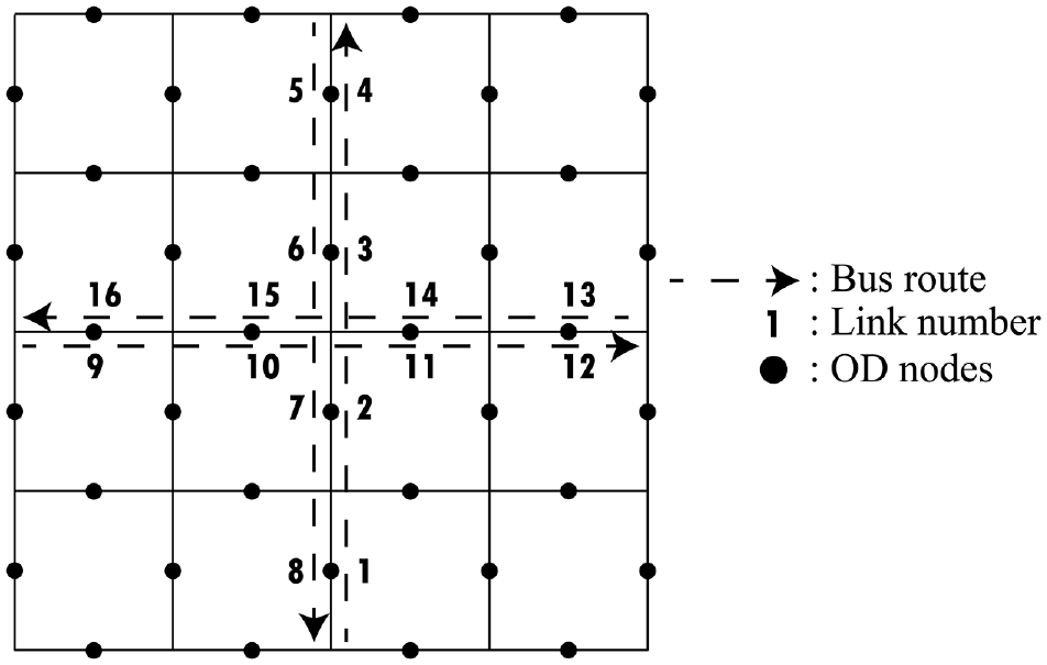
Test network for exploring linkages.

A demand pattern with 28,000 total trips per hour is used, which is enough to saturate the network without leading to oversaturation. The trip demand between each OD pair has a constant and a random component. The constant component is the same for all OD pairs, but the random component is a uniform random variable with a mean value of 20% of the constant component. As the network is a grid network, a larger number of shortest routes pass through center of the network than the periphery of the network. Thus, a distinctive congestion pattern is created by the constant part of the demand, such that the links closer to the central part of the network carry more volume than the links closer to the periphery of the network. The random part of the demand on the other hand is used to break the general symmetry of the network.

Dependency Problem

The dependency problem is demonstrated by determining the range of impacts a single DBL can have on car and bus travel times. Note that the implementation of DBLs can reduce bus delays but increase car travel times as a result of the reduction of capacity of a link (e.g., reducing the roadway from two to one lanes). To achieve this result, first a candidate link is chosen for DBL implementation. Then, two sets of scenarios are compared: (1) DBLs are implemented on all possible combinations of links except for the candidate link, and (2) DBLs are implemented on all possible combinations of links, as well as the candidate link. This comparison is done in a paired fashion and the difference in the total travel time by car and bus in the two scenarios is recorded. As a result, for each candidate bus lane location, 32,768 (2¹⁵) many different comparisons are made. The distribution of the percent difference between pairs of scenarios for a candidate DBL link for all possible combinations of links is created. The average, standard deviation, skew, minimum and maximum of this distribution is reported in Table 1. If there is no significant variance in the change in total travel time resulting from a DBL implementation depending on the location of existing DBLs, it can be assumed that the impact of implementing a DBL on that specific link is mostly independent of where other DBLs are located. Otherwise, it can be concluded that the impact of implementing a DBL on a given link largely depends on the existence of other DBLs on the network.

Table 1.

Distribution of Percent Change in Total Travel Time (TT) for Dedicated Bus Lane on Each Link

Link number	Min. TT (% change)	Max. TT (% change)	Avg. (% change)	SD	Skew
1	−2.77	2.22	−0.02	0.35	−0.31
2	− 3.11	4.10	0.47	0.83	− 0.16
3	− 1.90	4.60	0.61	0.80	0.44
4	−2.38	2.88	−0.04	0.18	0.03
5	−2.34	2.51	0.01	0.33	0.39
6	− 3.12	4.38	0.48	0.80	− 0.27
7	− 2.20	4.71	0.62	0.76	0.6
8	−2.10	2.51	−0.03	0.20	0.28
9	−2.67	2.60	0.03	0.35	0.4
10	− 3.72	3.23	0.22	0.76	− 0.37
11	− 2.40	4.59	0.52	0.77	0.59
12	−2.24	3.17	−0.04	0.20	1.36
13	−3.08	2.22	−0.04	0.35	−0.08
14	− 2.92	3.69	0.39	0.81	− 0.25
15	− 3.39	4.51	0.53	0.80	0.24
16	−2.20	2.24	−0.05	0.19	−0.06

Note: Min. = minimum; Max. = maximum; Avg. = average; SD = standard deviation. Optimum bus lane locations are shown in bold and italics.

Table 1 shows how the existence of DBLs located at other, different, locations influence the impact of a DBL at a given specific location. Furthermore, an enumeration of all possible DBL locations was conducted to determine the optimum solution, that is, the set of DBL locations that led to the lowest person delay. These solutions are shown in italics in Table 1. Looking at this table, implementing a DBL at a given location can have a range of impacts on the overall person delay depending on the location of the existing DBLs. Moreover, a specific DBL can increase or decrease the overall person delay depending on the location of the existing DBLs (in the range of −3.39%–4.60%). Note that although these percentages may appear small, this is the impact of a single DBL on the entire travel time. Further, as the results of LTM are deterministic, these differences are absolute, and not a margin of error.

The average impact for some DBL locations is close to zero for implementation of DBLs at certain locations (e.g., links 1, 4, 5, 8, 9, 12, 13, 16) with relatively small standard deviations, shown in bold. These are the DBL locations that have the smallest impact on person travel time, and thus they can reduce overall delay for a wider range of combinations of existing DBL locations. On the other hand, for other locations the average is greater than zero with a larger standard deviation (e.g., links, 2, 3, 6, 7, 10, 11, 14, 15), which implies that implementing DBLs to these locations is on average expected to increase overall total travel time. Overall, these results show that the decision variables of the DBL location selection problem are dependent on each other. Therefore, an algorithm that can account for the dependencies is needed to optimize DBL locations on a network.

Further, it can be seen that the links that are chosen for the optimal DBL location problem, shown in italics, all have mean values close to zero with relatively small standard deviation. This implies that the change in travel time expected from implementing DBL on these links is relatively stable. Thus, an optimization algorithm that can estimate the distributions presented in Table 1 can improve the optimum solution for the location selection problem, as these distributions contain important information on identifying the optimum locations of DBL implementation.

Solution Methods

This section describes possible methods to optimize the location of DBLs on a network, and discusses their effectiveness given the dependency problem. To determine the optimum location of the DBLs on a network a bi-level optimization method is used. The upper level of the optimization utilizes different heuristics to minimize the total in-vehicle travel time. The lower-level algorithm evaluates the total-in-vehicle travel time as the sum of the travel time by car and by obtained from the LTM as described previously. Note that the waiting time and walking time of bus passengers are not included in the objective function, as a DBL does not change these values. The decision variable is a vector consisting of 0 (no bus lane) or 1 (bus lane) for all possible bus lane locations. To solve this problem, a bi-level approach is used. The lower level uses the LTM as described to evaluate the network. The upper level uses one of four different optimization algorithms to determine the optimized bus lane locations: (1) Basic genetic algorithm (GA1), (2) Genetic algorithm with diversity control (GA2), (3) BOA, and (4) PBIL. The GAs are chosen because of their popularity in the transportation literature, and in solving the specific DBL location optimization problem (14 –18, 20 ). The BOA and PBIL are chosen as they can be used to estimate distributions and thus can help can account for dependencies between the decision variables.

Genetic Algorithms

The flowcharts of the two GAs are shown in Figure 2, a and b . The first GA (GA1) is a basic GA. It follows a simple selection, reproduction, mutation, and recombination cycle. First, a random set of solutions (i.e., vectors of DBL location configurations) is generated to create a population of solutions. Next, a tournament selection method is used ( 49 ) for selecting parents for generating the next population. In a tournament selection, first, a group of two chromosomes is picked randomly from the population. Then, the chromosome with the lower total travel time is selected from this pool as a parent. Tournament selection decreases the selection pressure on better chromosomes, thus increasing the likelihood of a more diverse population. After two parents are selected, two offspring chromosomes are created by a reduced surrogate crossover method. In the reduced surrogate crossover method, the crossing over, that is, swapping of the genes between the parents, is only done at cutting points where the genes differ between the two parents. Therefore, the chance of producing identical chromosomes is significantly reduced. Additionally, after the crossover is performed, a random mutation of a gene is applied with a five percent probability. Selection, reproduction, and mutation steps are repeated until all the offspring chromosomes are created. For the recombination step, where the next generation is created, the worse half of the population is replaced with the offspring population.

Figure 2.

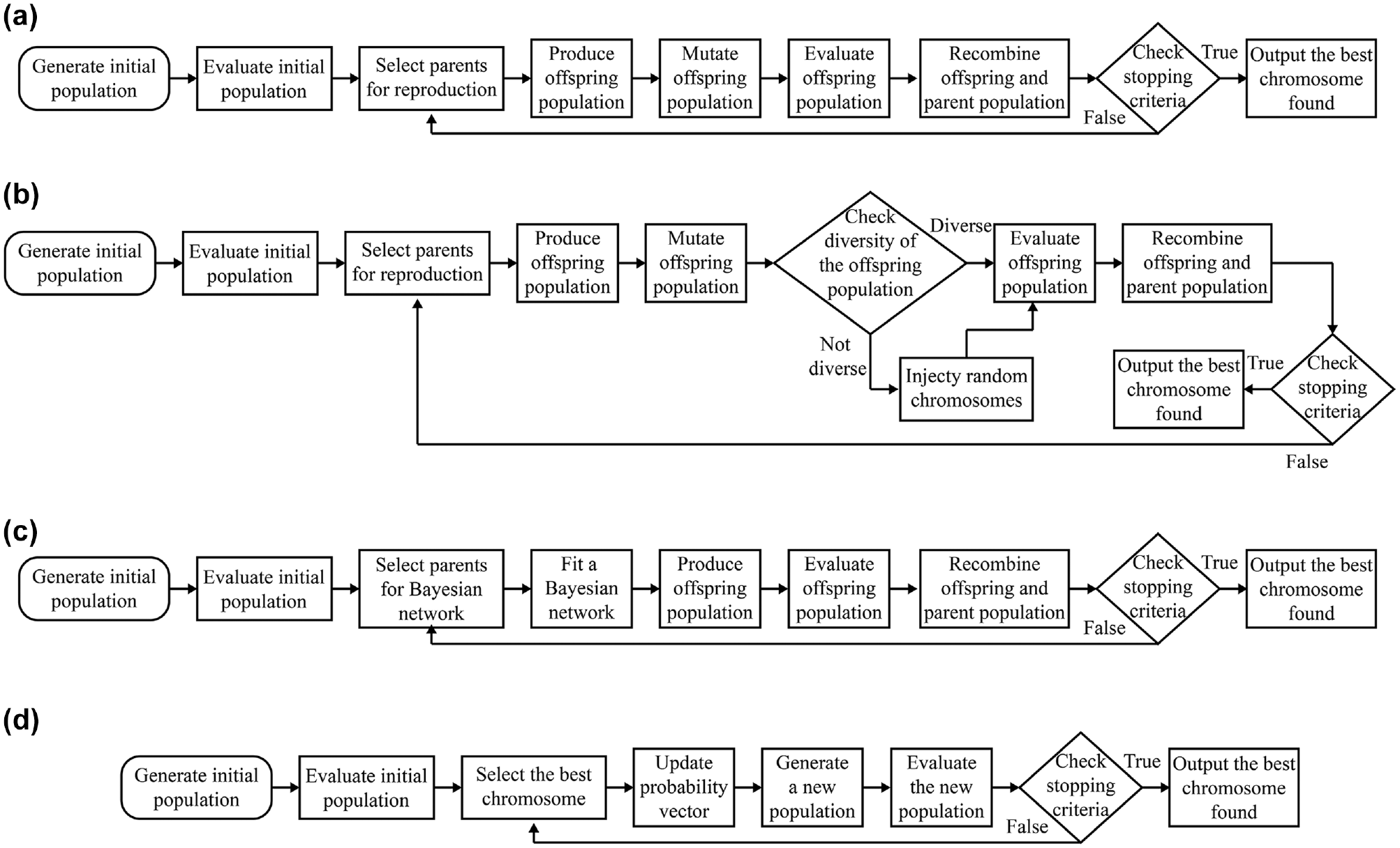
Flowcharts of: (a) GA1, (b) GA2, (c) BOA, and (d) PBIL.

The second GA (GA2) aims at increasing the diversity of the population. The only difference between GA1 and GA2 is the diversity management step. The selection, reproduction, mutation, and recombination methods used for GA2 are the same as the methods used for GA1. The purpose of the diversity management step is to detect a converged population and increase its diversity by forcing the algorithm to explore different areas of the solution space. The diversity check is done by calculating the average Hamming distance (i.e., number of different bits between two solutions) and checking the improvement of the best solution over the generations. This step of the algorithm is initiated if the best solution does not change for ten generations, and the population is not diverse. When it is initiated, half of the offspring chromosomes with the smallest Hamming distance (i.e., the chromosomes that are the most similar to each other) are replaced with randomly generated chromosomes. Note that, even though half of the offspring chromosomes are eliminated, the other half is still produced from the parent population. Therefore, the information from previous generations is not lost, and they can still guide the algorithm to a better solution.

Bayesian Optimization Algorithm

The BOA evolves a population of solutions by fitting and sampling of Bayesian networks. Unlike the GA, the BOA accounts for the dependent relationships between decision variables (i.e., locations of DBL implementations). Bayesian networks used in this algorithm represent the dependency structure between decision variables. Each node of a Bayesian network corresponds to a possible DBL location, and each directed edge of a Bayesian network represents a dependent relationship between locations of DBL implementations. The flowchart of the BOA is shown in Figure 2c.

Similar to the GA, an initial random population is generated, and future solution populations are selected from the current population using a tournament selection method. Next, a Bayesian network (i.e., a network of dependencies between decision variables) is fitted to the selected solutions using a search procedure to find the best Bayesian network that reflects the dependencies and independencies of the problem. The Bayesian network is constructed using a separate optimization algorithm within the BOA. The BOA uses a scoring metric to assess the quality of a Bayesian network structure, and a search procedure to test different network structures for a given scoring metric. In this study, the Bayesian information criterion (BIC) is used as a scoring metric ( 50 ). The BIC assumes that the number of dependencies in the network is proportional to the amount of compression of the data allowed by the network. Therefore, a Bayesian network structure that maximizes the BIC metric can be used to effectively describe the dependencies. The search procedure uses a simple greedy algorithm to learn the structure of the network. The process starts with a network with no edges (i.e., a network with no dependencies), then tests the change in the BIC metric for basic graph operations (edge addition, removal, and reversal). The operation that most increases the score is chosen. These two steps (testing and selecting operations) are repeated until the network can no longer be improved.

Next, offspring solutions are generated by sampling the fitted Bayesian network. In the Bayesian network, the variables (i.e., the presence of a DBL on a given link) can be categorized into three groups: (1) completely independent variables (i.e., no links are formed in the Bayesian network), (2) variables that depend on others, and (3) variables that others depend on (i.e., the value of the variables in group 2 that depend on the value of the variables in group 3). To sample from these sets of variables, a forward simulation is used ( 51 ). This sampling is done based on the conditional probabilities encoded in the Bayesian network, by assigning first the value (0—no bus lane, or 1—bus lane) for the independent variables (those in group 1), next assigning the value for the variables in group 3 (as the values of these do not depend on other variables) and finally by assigning the values of variables in group 2 (as their values depend on the values of the variables in group 3). The sampling process is repeated until all offspring solutions are generated.

Finally, the offspring solutions and the previous population are recombined by replacing the worse half of the population with the offspring solutions. The selection and recombination methods used in this algorithm are the same as the GAs.

Population-Based Incremental Learning

PBIL combines the generational evolution of GAs with competitive learning. The flowchart of the PBIL algorithm is shown in Figure 2d. The main difference between PBIL and the other algorithms tested is that there is no parent–offspring relationship between consecutive generations. A probability vector, $P$ , consisting of the probability of implementing a DBL on each link is used to generate an entire new population of solutions. The probability vector is updated and mutated after evaluation of each new population, as shown in Equations 5 and 6.

P_{i}^{t + 1} = (P_{i}^{t} \times (1 - LR)) + (V_{i}^{t} \times LR)

(5)

P_{i, mutated}^{t + 1} = P_{i}^{t + 1} (1 - Δ m) + rand (0, 1) \times Δ m

(6)

where $P_{i}^{t}$ is the probability of implementing a DBL on link $i$ in generation $t$ , $LR$ is the learning rate, and $V_{i}^{t}$ is the value (0 or 1) of the $i$ th position of the best solution found in generation, $t$ . The new generation of solutions is created by randomly sampling the solution space weighted by the probability vector. Therefore, Equation 5 moves future solutions toward the best solution found in the current generation. Similar to other methods tested, the probability vector converges around a solution as the search progresses. However, unlike GAs, the PBIL allows explicit control of the speed of convergence with the learning rate parameter, $LR$ . The learning rate parameter enables the PBIL to explore a larger portion of the solution space, which is essential for problems with dependencies, before starting to converge to a solution. The value of the LR creates a balance between the portion of the solution space explored and the convergence speed. The mutation operator, see Equation 6, is also responsible for expanding the explored solution space by shifting the probabilities with a magnitude of $Δ m$ in the probability vector. Mutation only happens with a predefined mutation probability. Notice that, different from GAs, the mutation is applied to the probability vector instead of to individual solution vectors.

Network and Experiment Setup

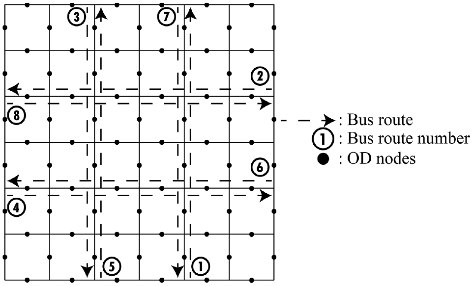
The four optimization algorithms described in the previous section are tested using a 7 × 7 symmetrical grid network shown in Figure 3. There are a total of eight bus routes, each of length 2.4 km (corresponding to six links) that run east/west and north/south, see Figure 4. For this network, the decision variable is a $48 \times 1$ vector consisting of 0 (no bus lane) or 1 (bus lane) for all possible DBL links. The network parameters (jam density, capacity, link length, free-flow speed, signal settings, bus headway, and walking speed) are the same as in the linkage problem section.

Figure 3.

Test network for exploring use of different algorithms.

Figure 4.

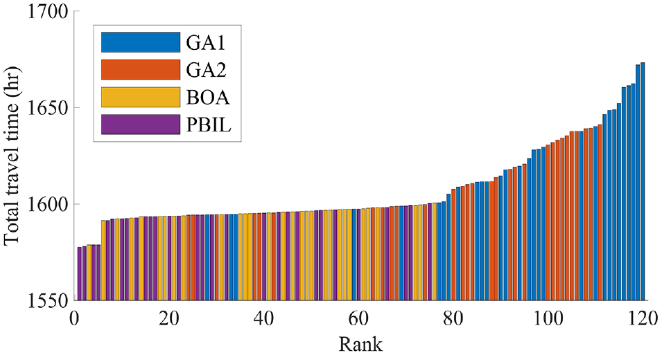
Ranked results of all optimization instances.

The average total trip demand in the network, equal to 48,800 vehicles per hour, is chosen such that a network without DBLs is saturated. The trip demand between each OD pair has a constant and a random component, similar to that described in the linkage problem section.

The modal split model used in the LTM calibrated to create a 6% modal shift from cars to buses when DBLs are implemented on all potential links. The values of parameters used in Equations 2 and 3 are $C_{car} = 50$ , $C_{bus} = 54.1$ , and $a_{car} = a_{bus} = 0.5$ . For the route selection model (see Equation 4), the sensitivity parameter, $a$ , is set to $2.33$ to limit the unnecessary detours. The car total travel time (in-vehicle), bus total travel time (in-vehicle), and modal split values for the no DBL and full DBL scenarios are shown in Table 2.

Table 2.

Results of No Dedicated Bus Lane (DBL) and Full DBL Cases

	Total bus travel time (TT) (Avg. bus TT)	Total car TT (Avg. car TT)	Total TT	Bus mode share (%)
No DBL (baseline)	603 h (3.9 min)	1,316 h (4.9 min)	1919 h	30
Full DBL	508 h (2.9 min)	1,309 h (5.5 min)	1817 h	36

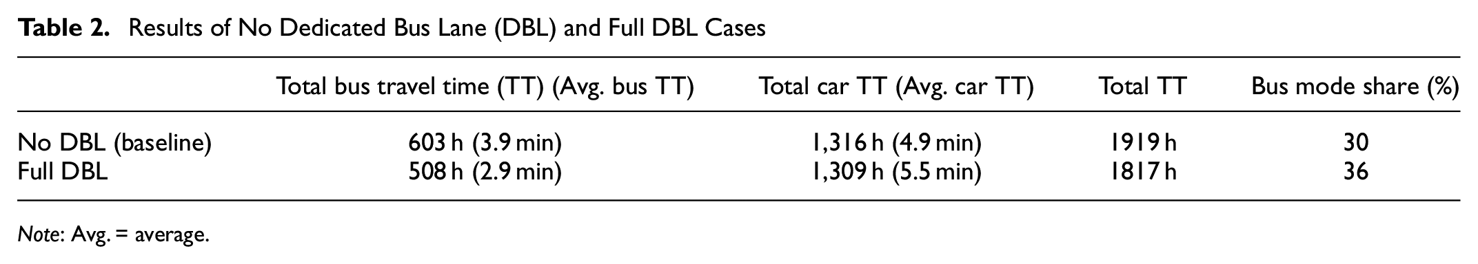
Note: Avg. = average.

The trade-off between the decrease in bus delay and the increase in car delay can be seen in Table 2. Note that as the bus network does not completely cover the whole network, the average travel distance by bus is shorter than by car. Therefore, the average travel time by bus is lower than by car, too. When DBLs are implemented, the car travel time increases by 12%, and the bus travel time decreases by 25%. Overall, this corresponds to a decrease in total travel time of 5%, even though there are fewer bus users than car users. The decrease in total travel time, despite the increase in car travel time, can be attributed to the mode shift, that is, the 6% mode shift from cars to buses removes enough cars from traffic to offset the delay increase caused by the reduction in car capacity. Even though implementing DBLs at all possible locations can improve the total travel time compared with the baseline scenario, it is not the optimum solution in relation to total travel time for the location selection problem. Given that the bus travel time, car travel time, capacity, and mode shift directly affect each other, it is possible that a set of DBL locations can reduce the total travel time more than the full DBL case. The expectation is that this optimum combination of DBL locations would facilitate a mode shift by only reducing the bus travel time without significantly increasing car delay.

The parameters used for each optimization algorithm are listed in Table 3. Note that the parameters are set to achieve comparable computation times among the algorithms. Although the computational efforts of the algorithms themselves are not the same, the major determinant of the computational time is the number of evaluations of the test network, as each LTM run is relatively computationally expensive. Each optimization algorithm is run 30 times, and for each optimization instance, 4,000 individual solutions are created over 100 generations. The consistent value of 4,000 individual solutions ensures that the computation time of each algorithm is similar. The GA algorithms, along with BOA, have a recombination step which implies that in each generation half the population is the same as the previous generation (and does not require evaluation). Therefore, to generate 4,000 solutions a population size of eighty is needed for these algorithms. On the other hand, the PBIL generates an entirely new population in each generation and so a population size of forty suffices to generate 4,000 solutions. The performance of each optimization algorithm is compared with each other in relation to consistency and quality of the solutions, and exploration capability of each algorithm.

Table 3.

Parameters of Each Optimization Algorithm

	GA1	GA2	BOA	PBIL
Population size	80	80	80	40
Mutation probability	0.05	0.05	na	0.05
Tournament size	2	2	2	na
Learning rate	na	na	na	0.1
Mutation shift	na	na	na	0.05
Stopping criteria	100 generations	100 generations	100 generations	100 generations

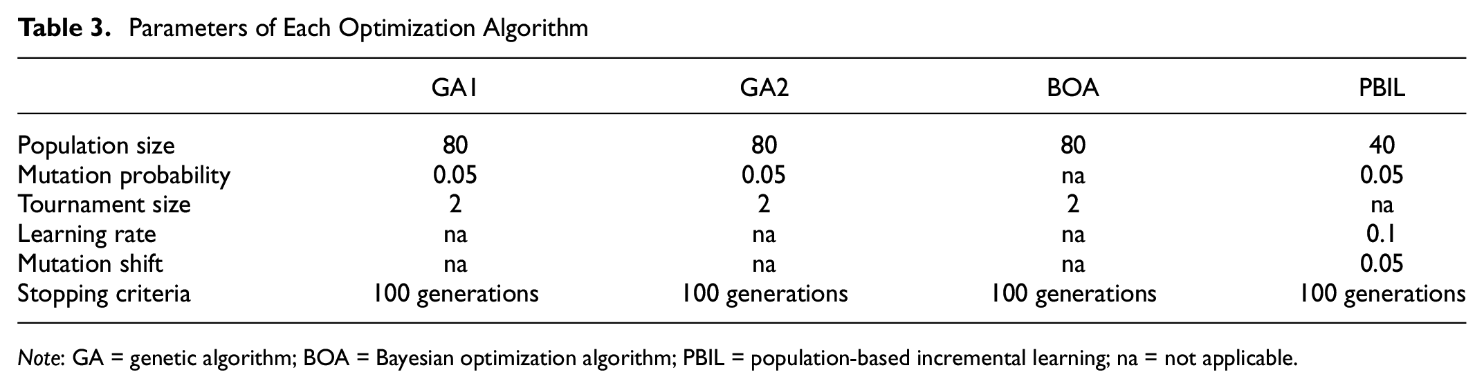
Note: GA = genetic algorithm; BOA = Bayesian optimization algorithm; PBIL = population-based incremental learning; na = not applicable.

All four algorithms are coded in MATLAB and a PC with a 12-core AMD Ryzen 3900x CPU was used to run the codes. On average, each optimization instance took less than 4 h to complete. It should be noted that the computation time is dominated by the lower-level evaluation (i.e., LTM model). Thus, as the number of lower-level evaluations for each algorithm is same and equal to 4,000, the run time of each algorithm is almost the same.

Results

In this section, the optimization performance of the GA1, GA2, PBIL, and BOA are compared. First, the solutions found by each optimization algorithm are compared considering the value of the optimum minimum total travel time on the test network, and the common spatial characteristics of the optimum DBL configurations found by the algorithms. Then, the capability of each algorithm in exploring the solution space is compared according to the number of unique evaluations, the number of objective value improvements over the solution duration, and the number of generations to convergence in a single optimization instance.

Comparison of Solutions Found by the Algorithms

To compare the solutions found by the optimization algorithms, each optimization algorithm is run 30 times. The solutions found by the algorithms are first compared considering travel times, and next the optimum solutions are compared spatially.

Travel Time Comparison

The maximum, minimum, and average of the total travel times found as the optimal solution are shown in Table 4. From this table, the BOA and PBIL are able to find better solutions than the GA1 and GA2. This is further investigated in Figure 4, which shows the ranked optimum total travel time values obtained from these 120 optimizations runs. Figure 4 reveals that the worst nine solutions are obtained from the GA1. Given that the GA1 is the most basic form of the GAs, and it does not have a mechanism either to learn linkages or to keep the population diverse enough to explore a large part of the solution space, this result is not surprising. Although the GA1 found decent solutions in some optimization instances, results show that the overall performance of the GA1 is unreliable. The GA2 performed better than the GA1 as a result of the diversity management step. However, the results of GA2 are also inconsistent compared with the results of BOA and PBIL. Overall, the worst forty-five solutions are found by the GA1 and GA2. Overall, the range of the optimum travel times found from these algorithms is rather large (1,594–1,673 h). The best performing algorithms are the BOA and the PBIL. Both algorithms consistently found better solutions than the GAs and the top twenty solutions are found by either the BOA or the PBIL. The performance difference between the BOA and the PBIL is negligible, and the range of the optimum total travel times found from these algorithms is rather narrow (1,578–1,600 h).

Table 4.

Range of Resulting Total Travel Time Values (in hours) for Each Optimization Algorithm

	GA1	GA2	BOA	PBIL
Minimum	1,594	1,594	1,579	1,578
Average	1,627	1,615	1,595	1,593
Maximum	1,673	1,641	1,601	1,600

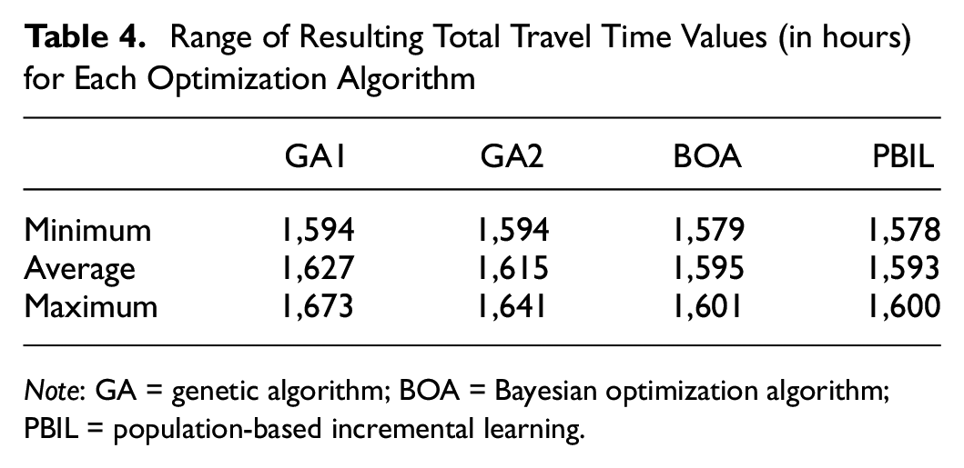
Note: GA = genetic algorithm; BOA = Bayesian optimization algorithm; PBIL = population-based incremental learning.

Table 5 shows the total car travel time, total bus travel time, and the modal split values for the top three optimization results, where the top two results are found by the PBIL and the third is found by the BOA. The results suggest that the travel time values of these configurations are similar to each other. Next, these three results are compared spatially.

Table 5.

Results of No Dedicated Bus Lane (DBL), Full DBL, and Best Three Optimization Instances

	Total bus travel time (TT) (Avg. bus TT)	Total car TT (Avg. car TT)	Total TT	Bus share (%)
No DBL (baseline)	603 h (3.9 min)	1,316 h (4.9 min)	1,919 h	30
1st configuration	471 h (3.0 min)	1,107 h (4.7 min)	1,578 h	33
2nd configuration	472 h (3.0 min)	1,106 h (4.7 min)	1,578 h	33
3rd configuration	468 h (3.0 min)	1,111 h (4.7 min)	1,579 h	33
Full DBL	508 h (2.9 min)	1,309 h (5.5 min)	1,817 h	36

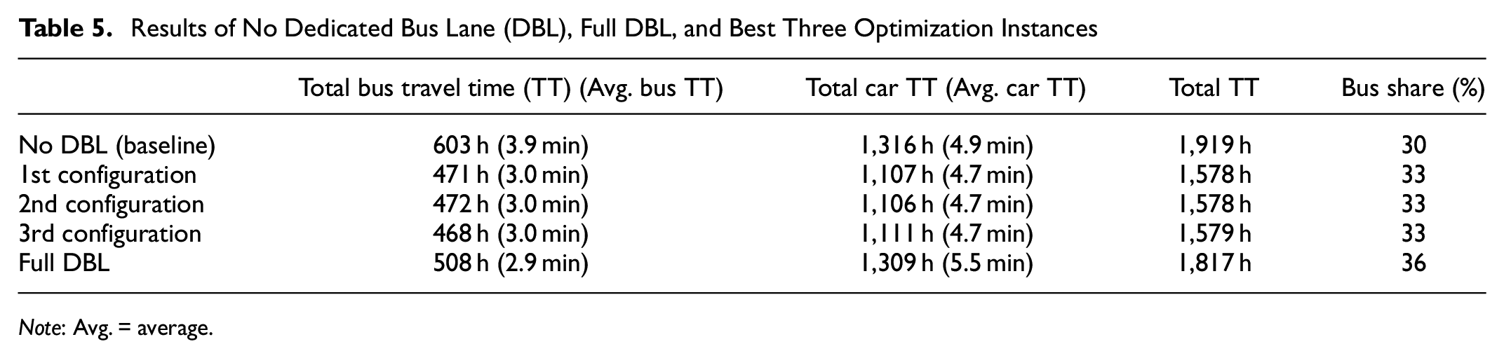
Note: Avg. = average.

Spatial Comparison of Optimal Results

The DBL configurations for the top three optimization results are shown in Figure 5. As can be seen from Figure 5, share similar spatial characteristics. These results suggest that to minimize total travel time, the algorithms avoid implementing DBLs on central links. These links on the central portion of the network carry higher car and bus passengers flow than the rest of the network. Therefore, implementing DBLs on these links provides the largest delay savings to bus passenger. However, the car delay significantly increases if DBLs are implemented on these central links, as the car volume is large. Thus, implementing DBLs to these locations is likely to increase the total travel time of the network users. As the objective of the optimization is to minimize the total travel time, it is expected that the optimization algorithms avoid the solutions that contain the central portion of the network. This is an expected result, as to minimize total travel time the DBLs need to be implemented on links where they can create a mode shift without significantly affecting car traffic. Considering Table 5, all three DBL configurations not only improved the bus travel (in-vehicle) time but also slightly decreased the average car travel (in-vehicle) time by creating a three percent mode shift from cars to buses. Compared with the full DBL implementation, these optimum DBL locations can reduce bus delays nearly as much, with significantly lower car travel times.

Figure 5.

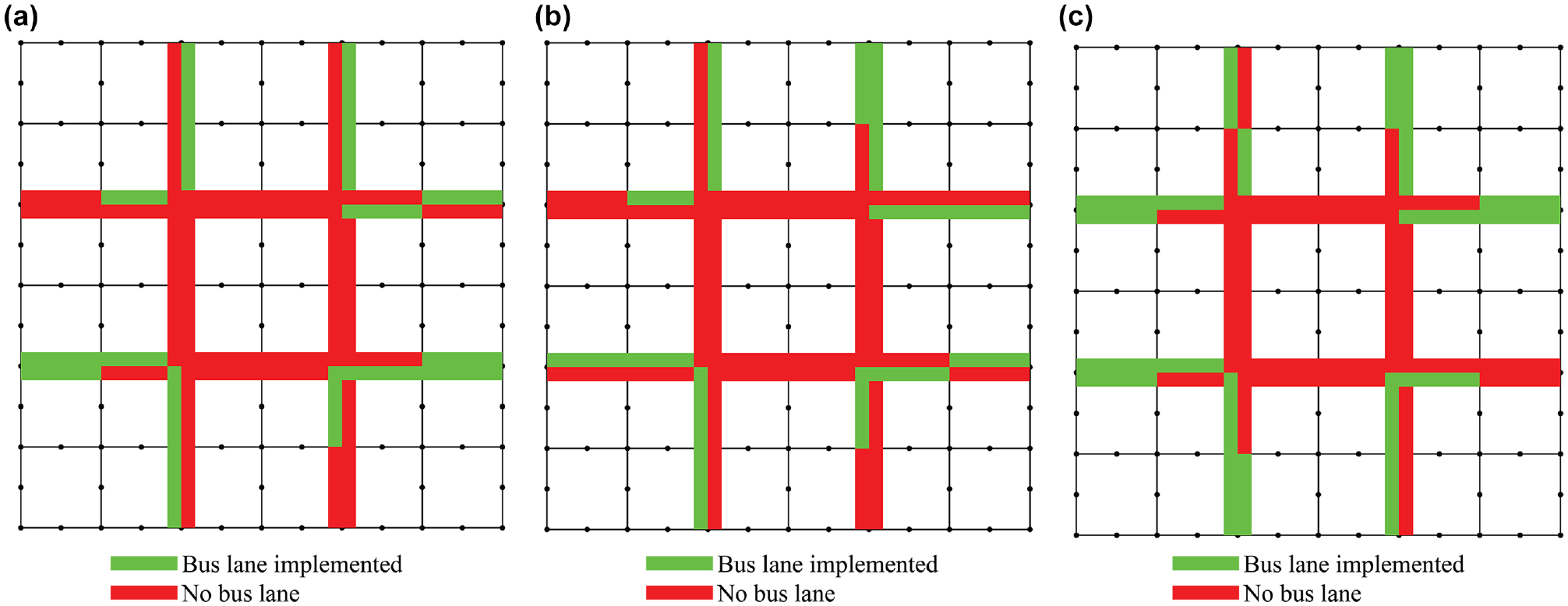
The dedicated bus lane configurations of the best three optimization instances: (a) best configuration, (b) second best configuration, and (c) third best configuration.

Figure 6 shows a frequency heat map of the number of runs of the optimization algorithm that finds that a DBL should be implemented on a given link in the optimum solution. More yellow rectangles indicate a higher frequency of DBLs being implemented, whereas more blue rectangles indicate a lower frequency. This figure can be used to identify the commonalities among the solutions found for the different solution algorithms. Most of the optimum solutions found from the different algorithms avoid DBL implementation to the central links to minimize the total travel time. However, as seen from Figure 6, a and b , some of the GA1 and GA2 results include links from the central network, whereas solutions found from PBIL and BOA always avoided that region. On inspection of the results of the individual optimization instances, it is found that the worst-performing solutions found by GA1 and GA2 are the solutions that contain links from the central part of the network.

Figure 6.

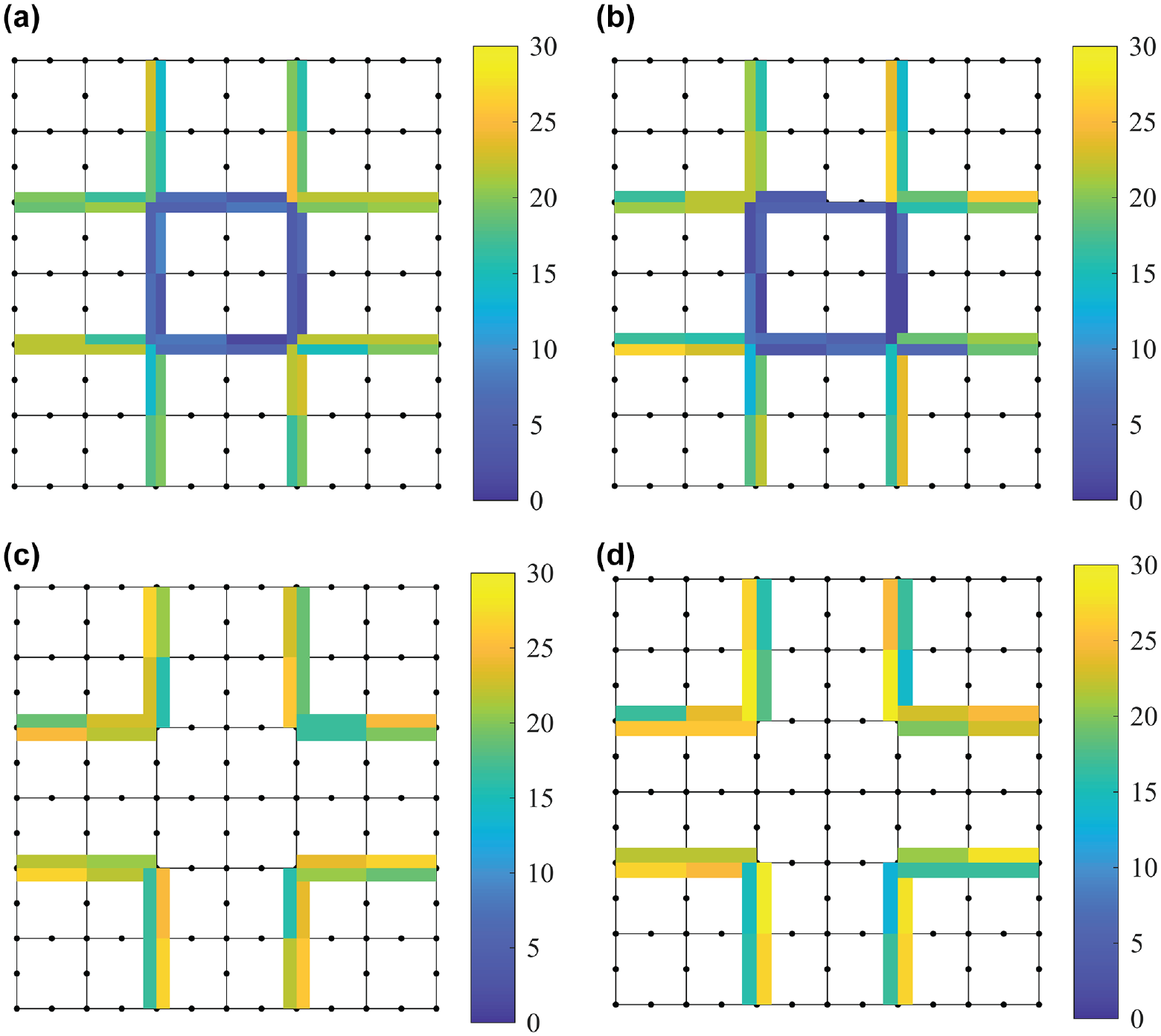
Heat map showing common dedicated bus lane implementation locations found from 30 optimization instances of (a) GA1, (b) GA2, (c) PBIL, and (d) BOA.

On the other hand, the GA1 and GA2 find a more varied set of optimum DBL locations for the outer links as the result of each run (average Hamming distance between solutions is 0.79 and 0.71, respectively), whereas the PBIL and BOA are more consistent in their solutions (average Hamming distance between solutions is 0.51 and 0.45, respectively). Also, the links found in the best solution as described above are frequently found in the configurations found by the PBIL and BOA.

Exploration of Each Algorithm

For each algorithm used, there is an initial exploration phase followed by a phase that is aimed at fine-tuning the solution. The exploration phase is when the algorithms create a variety of different solutions to explore the solution space with the goal of identifying the general region within the solution space that the optimal solution may located. Next, all the algorithms shift to the exploitation of the locality phase, where the goal is to find a good solution within a small area of the solution space. This dual functionality is the basic mechanics of all evolutionary algorithms. However, without enough exploration in the initial phase, it is likely that these algorithms are likely to exploit a sub-optimal part of the solution space.

In this section, the capability of the algorithm to explore the solution space is investigated by comparing the different runs of each algorithm using three metrics:

(1) The number of unique solutions evaluated in an optimization run of 100 generations (i.e., over the 4,000 total solutions evaluations),

(2) The number of generations in which the best solution was improved in an optimization run of 100 generations, and

(3) The generation number in which the final optimum solution first appeared in the solution space of the optimization run.

These metrics are calculated for thirty different runs of each algorithm, and the maximum, minimum and average values over these thirty runs for the above metrics for each algorithm are shown in Table 6.

Table 6.

Number of Unique Evaluations, Number of Generations in Which the Best Solution Improved and the Generation Number in Which the Final Optimum Solution First Appeared

	GA1	GA2	BOA	PBIL
Number of unique evaluations
Minimum	284	750	1,178	2,579
Average	435	1,454	1,477	2,985
Maximum	635	2,025	2,028	3,661
Number of generations in which the best solution improved
Minimum	7	11	8	11
Average	15	19	16	20
Maximum	25	30	24	34
The generation number in which the best solution first appeared
Minimum	9	35	19	37
Average	61	81	44	72
Maximum	98	100	99	97

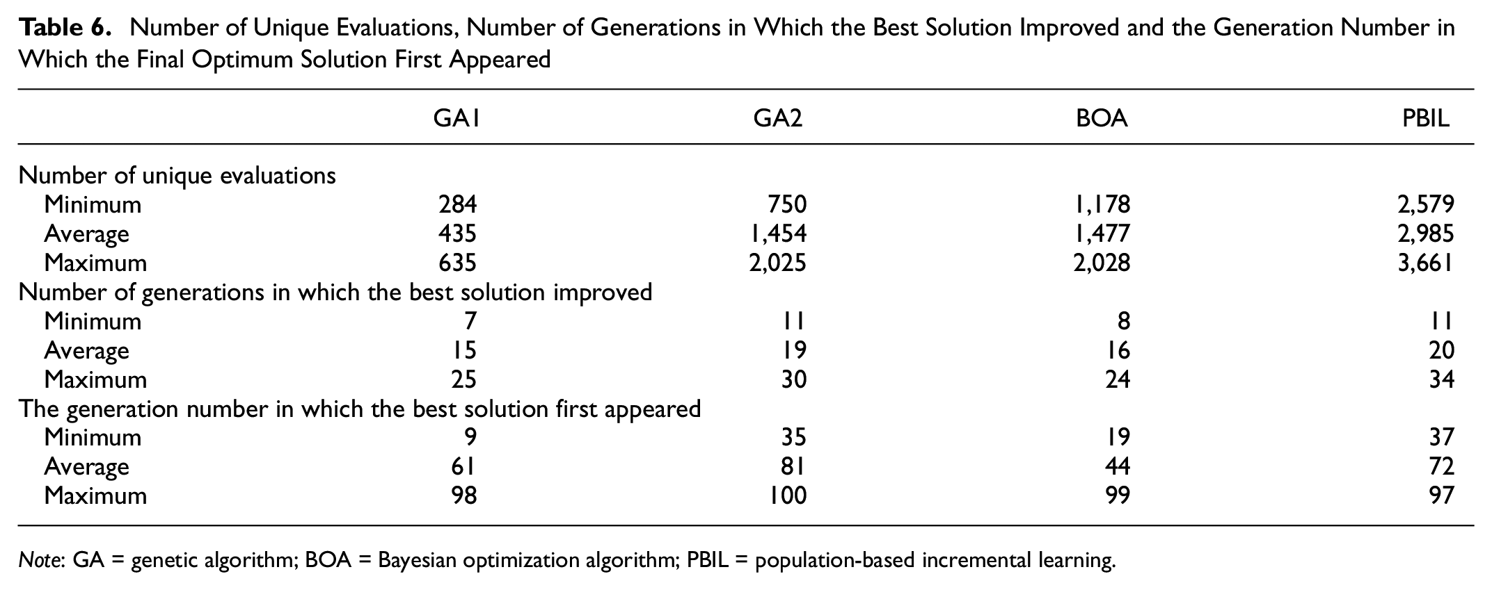
Note: GA = genetic algorithm; BOA = Bayesian optimization algorithm; PBIL = population-based incremental learning.

Looking at Table 6, it can be seen that the GA1 evaluated the least number of unique solutions, whereas the GA2 and the BOA evaluated a similar number of unique solutions approximately three times larger than that of the GA1. This shows that the diversity management step increased the exploration capability of GA2 as compared with the GA1. Because of the increased exploration capability, GA2 improved the best solution more frequently than GA1. On inspection of the results of individual population instances, it is found that the GA1 often converged prematurely and relied on the mutation operator for generating better solutions. However, as the GA2 does not have a mechanism to learn linkages, this increased exploration capability did not result in better solutions.

On the other hand, the PBIL evaluated the greatest number of unique solutions, approximately 104% more than the GA2 and the BOA. The main reason for this superior exploration capability is that the PBIL produces an entirely new population at each generation by using the probability vector. PBIL’s superior exploration capability can also be seen in Table 6. PBIL improved the best solution more frequently than any other algorithms. However, the exploration focus of the PBIL diminishes the exploitation capability of the algorithm ( 52 ), resulting in slower convergence. On average, the best solution in an optimization instance first appeared in the population in the later stages of the optimization (most of the time, more than halfway through the optimization). The exploitation capability of the PBIL can be enhanced by increasing the learning rate parameter ( $LR$ ). However, as the DBL location selection problem is a problem with dependencies, increasing the learning rate can result in the premature convergence of the solution.

The BOA was able to find solutions as good as the ones found by the PBIL by evaluating only half of the unique solutions that the PBIL evaluated. Moreover, the BOA can on average find the final optimum solution in the least number of iterations out of all the algorithms. This is because the BOA exploits the dependencies among the solutions to identify the optimum solution. As BOA utilizes Bayesian networks to learn the linkages among solutions, both the exploration and exploitation processes are more guided than the other algorithms.

Discussion and Concluding Remarks

This study examined the dependency problem in the mathematical optimization of transportation networks. First, the dependency problem in the selection of the optimum location of DBLs on a small network is illustrated by enumerating all possible DBLs location configurations. Results show that the performance in relation to impacts on bus and car travel times of a given DBL depends on where other DBLs exist. Therefore, a linkage exists between locations of DBLs on a network. Although this work only considered the DBL location selection problem, other transportation network optimization problems that involve capacity-changing modifications are likely to have similar linkage problems. After the illustration of the linkage problem, the performance of two evolutionary algorithms that are more capable of linkage learning compared with GAs that are widely used in transportation literature are explored.

Results show that both PBIL and BOA perform better than the tested GAs. These two algorithms can explicitly account for the dependencies in the solution space and therefore can guide the algorithm to a better solution. As expected, the basic GA (GA1) performed the worst among the tested algorithms as its exploration capability is significantly worse than other algorithms, and often converged prematurely. On the other hand, because of the diversity management step, the modified GA (GA2) explored a much larger portion of the solution space and found better solutions than GA1. However, the solutions found from GA2 had a much larger range as compared with the solutions found from BOA and PBIL. BOA and PBIL performed similarly in relation to the total travel time of the solutions they found. Out of a total of thirty runs of GA1, GA2, PBIL and BOA each, the top twenty are found by BOA and PBIL. However, BOA required fewer generations and less exploration than PBIL to find the solutions. When all results considered, BOA performed best among all tested algorithms.

In this study, BOA and PBIL are selected as an alternative solution method to GAs to identify methods that are capable of learning the linkage between decision variables better than GAs. Of course, the performance of a metaheuristic algorithm would be subject to features that are problem specific and algorithm specific, such as the structure of the optimization problem and selection of algorithm parameters. Also, with enough computational power and fine-tuning of an optimization algorithm, most of the metaheuristic methods can find a reasonably good solution to an optimization problem. However, for optimization problems that require computationally expensive solution evaluation methods, such as microsimulation or LTM, the number of iterations required to find a good solution becomes important for practitioners. Although GAs are easier to implement and more intuitive to work with, using more advanced metaheuristics can save time and significantly improve the solutions found.

Even though the methods are flexible, the results are limited to the few test scenarios shown in this paper. Future work can consider different shapes and types of networks, travel time, and demand stochasticity, and further test different algorithms for accounting for the dependencies in networks. However, it is expected that the dependency problem exists for all transportation networks, and that heuristic algorithms that explicitly account for this dependency, such as BOA and PBIL, can perform better for other transportation networks and other location selection problems.

Footnotes

Author Contributions

The authors confirm contribution to the paper as follows: study conception and design: M. Bayrak, S. I. Guler; data collection: M. Bayrak, S. I. Guler; analysis and interpretation of results: M. Bayrak, S. I. Guler; draft manuscript preparation: M. Bayrak, S. I. Guler. All authors reviewed the results and approved the final version of the manuscript.

Declaration of Conflicting Interests

The author(s) declared no potential conflicts of interest with respect to the research, authorship, and/or publication of this article.

Funding

The author(s) received no financial support for the research, authorship, and/or publication of this article.

ORCID iDs

Murat Bayrak

S. Ilgin Guler

References

Green Wave Traffic Control System Optimization Based on Adaptive Genetic-Artificial Fish Swarm Algorithm. Neural Computing and Applications, Vol. 31, 2019, pp. 2073–2083.

Gupta

Sharma

Reddy

Kumar

Panigrahi

B. K.

Traffic Signal Coordination Using Termite Spatial Correlation Optimization for Oversaturated Signals. Proc., IEEE International WIE Conference on Electrical and Computer Engineering (WIECON-ECE), Dehradun, India, 2017.

Ceylan

Bell

M. G. H.

Traffic Signal Timing Optimisation Based on Genetic Algorithm Approach, Including Drivers’ Routing. Transportation Research Part B: Methodological, Vol. 38, 2004, pp. 329–342.

Tan

M. K.

Chuo

H. S. E.

Chin

R. K. Y.

Yeo

K. B.

Teo

K. T. K.

Genetic Algorithm Based Signal Optimizer for Oversaturated Urban Signalized Intersection. Proc., IEEE International Conference on Consumer Electronics-Asia (ICCE-Asia), Seoul, South Korea, 2016.

Shepherd

Sumalee

A Genetic Algorithm Based Approach to Optimal Toll Level and Location Problems. Networks and Spatial Economics, Vol. 4, 2004, pp. 161–179.

González Velarde

J. L.

Camacho-Vallejo

J.-F.

Pinto Serrano

A Scatter Search Algorithm for Solving a Bilevel Optimization Model for Determining Highway Tolls. Computación y Sistemas, Vol. 19, 2015, pp. 5–16.

Brotcorne

Labbé

Marcotte

Savard

A Bilevel Model for Toll Optimization on a Multicommodity Transportation Network. Transportation Science, Vol. 35, 2001, pp. 345–358.

Koh

Solving Transportation Bi-Level Programs With Differential Evolution. Proc., IEEE Congress on Evolutionary Computation, Singapore, 2007.

Liu

B. Z.

Y. E.

Cao

Jiang

Meng

Liu

Gao

Optimizing a Desirable Fare Structure for a Bus-Subway Corridor. PLoS One, Vol. 12, 2017.

10.

Yamada

Russ

B. F.

Castro

Taniguchi

Designing Multimodal Freight Transport Networks: A Heuristic Approach and Applications. Transportation Science, Vol. 43, 2009, pp. 129–143.

11.

Mathew

T. V.

Sharma

Continuous Network Design With Emission Pricing as a Bi-Level Optimization Problem. Proc., 9th International Conference on Applications of Advanced Technology in Transportation (AATT)Transportation, Chicago, IL, 2006.

12.

Fan

Machemehl

R. B.

Bi-Level Optimization Model for Public Transportation Network Redesign Problem: Accounting for Equity Issues. Transportation Research Record: Journal of the Transportation Research Board, 2011. 2263: 151–162.

13.

Poorzahedy

Rouhani

O. M.

Hybrid Meta-Heuristic Algorithms for Solving Network Design Problem. European Journal of Operational Research, Vol. 182, 2007, pp. 578–596.

14.

Chen

An Optimization Model for the Selection of Bus-Only Lanes in a City. PLoS One, Vol. 10, 2015.

15.

Mesbah

Sarvi

Currie

Optimization of Transit Priority in the Transportation Network Using a Genetic Algorithm. IEEE Transactions on Intelligent Transportation Systems, Vol. 12, 2011, pp. 908–919.

16.

Yao

Shi

Zhou

Qin

Combinatorial Optimization of Exclusive Bus Lanes and Bus Frequencies in Multi-Modal Transportation Network. Journal of Transportation Engineering, Vol. 138, 2012, pp. 1422–1429.

17.

Mesbah

Sarvi

Currie

Saffarzadeh

Policy-Making Tool for Optimization of Transit Priority Lanes in Urban Network. Transportation Research Record: Journal of the Transportation Research Board, 2010. 2197: 54–62.

18.

Bingfeng

Ming

Xiaobao

Ziyou

Bi-Level Programming Model for Exclusive Bus Lanes Configuration in Multimodal Traffic Network. Transportation Research Procedia, Vol. 25, 2017, pp. 652–663.

19.

Kong

Sun

Yao

Gao

A Bi-Level Programming for Bus Lane Network Design. Transportation Research Part C: Emerging Technologies, Vol. 55, 2015, pp. 310–327.

20.

Bayrak

Guler

S. I.

Optimization of Dedicated Bus Lane Location on a Transportation Network While Accounting for Traffic Dynamics. Public Transport, Vol. 13, 2021, pp. 325–347.

21.

Mesbah

Sarvi

Ouveysi

Currie

Optimization of Transit Priority in the Transportation Network Using a Decomposition Methodology. Transportation Research Part C: Emerging Technologies, Vol. 19, No. 2, 2011, pp. 363–373.

22.

Sun

Combinatorial Optimization of Bus Lane Infrastructure Layout and Bus Operation Management. Advances in Mechanical Engineering, Vol. 9, 2017.

23.

Petit

Yildirimoglu

Geroliminis

Ouyang

Dedicated Bus Lane Network Design Under Demand Diversion and Dynamic Traffic Congestion: An Aggregated Network and Continuous Approximation Model Approach. Transportation Research Part C: Emerging Technologies, Vol. 128, 2021.

24.

Goldberg

D. E.

Genetic Algorithms and Walsh Functions: Part I, a Gentle Introduction. Complex Systems, Vol. 3, 1989, pp. 129–152.

25.

Goldberg

D. E.

Genetic Algorithms and Walsh Functions: Part II, Deception and its Analysis. Complex Systems, Vol. 3, 1989, pp. 153–171.

26.

Kennedy

P. J.

Osborn

T. R.

A Double-Stranded Encoding Scheme With Inversion Operator for Genetic Algorithms. Proc., 3rd Annual Conference on Genetic and Evolutionary Computation, San Francisco, CA, 2001.

27.

Levenick

Metabits: Generic Endogenous Crossover Control. Proc., Sixth International Conference on Genetic Algorithms, Pittsburgh, PA, 1995.

28.

Schaffer

J. D.

Morishima

An Adaptive Crossover Distribution Mechanism for Genetic Algorithms. Proc., Genetic Algorithms and their Applications: Proceedings of the Second International Conference on Genetic Algorithms, Cambridge, MA, 1987.

29.

Louis

S. J.

Rawlins

G. J. E.

Designer Genetic Algorithms: Genetic Algorithms in Structure Design. Proc., International Conference on Genetic Algorithms (ICGA), San Diego, CA, 1991.

30.

Eshelman

L. J.

Schaffer

J. D.

Productive Recombination and Propagating and Preserving Schemata. Foundations of Genetic Algorithms, Vol. 3, 1995, pp. 299–313.

31.

White

Oppacher

Adaptive Crossover Using Automata. Proc., International Conference on Parallel Problem Solving From Nature, Jerusalem, Israel, 1994.

32.

Vekaria

Clack

Selective Crossover in Genetic Algorithms: An Empirical Study. Proc., International Conference on Parallel Problem Solving From Nature, Amsterdam, The Netherlands, 1998.

33.

Smith

Fogarty

T. C.

An Adaptive Poly-Parental Recombination Strategy. Proc., AISB Workshop on Evolutionary Computing, Sheffield, 1995.

34.

Salman

A. A.

Mehrotra

Mohan

C. K.

Linkage Crossover for Genetic Algorithms. Proc., 1st Annual Conference on Genetic and Evolutionary Computation-Volume 1, Orlando, FL, 1999.

35.

Greene

W. A.

A Genetic Algorithm With Self-Distancing Bits But No Overt Linkage. Proc., 4th Annual Conference on Genetic and Evolutionary Computation, New York, NY, 2002.

36.

Goldberg

D. E.

Korb

Deb

Messy Genetic Algorithms: Motivation, Analysis, and First Results. Complex Systems, Vol. 3, 1989, pp. 493–530.

37.

Goldberg

D. E.

Deb

Kargupta

Harik

G. R.

Rapid Accurate Optimization of Difficult Problems Using Fast Messy Genetic Algorithms. Proc., International Conference on Genetic Algorithms (ICGA), Urbana-Champaign, IL, 1993.

38.

Kargupta

The Gene Expression Messy Genetic Algorithm. Proc., IEEE International Conference on Evolutionary Computation, Nagoya, Japan, 1996.

39.

Burke

D. S.

De Jong

K. A.

Grefenstette

J. J.

Ramsey

C. L.

A. S.

Putting More Genetics into Genetic Algorithms. Evolutionary Computation, Vol. 6, 1998, pp. 387–410.

40.

Pelikan

Mühlenbein

The Bivariate Marginal Distribution Algorithm. In Advances in Soft Computing ( Roy

Furuhashi

Chawdhry

P. K.

, eds.), Springer, London, 1999, pp. 521–535.

41.

Baluja

Population-Based Incremental Learning. A Method for Integrating Genetic Search Based Function Optimization and Competitive Learning. Technical Report CMU-CS-94-163, Carnegie Mellon University, Pittsburgh, PA, 1994.

42.

Sastry

Goldberg

D. E.

On Extended Compact Genetic Algorithm. IlliGAL Report. Illinois Genetic Algorithms Laboratory (IlliGAL), Urbana, IL, 2000.

43.

Mühlenbein

Mahnig

FDA-A Scalable Evolutionary Algorithm for the Optimization of Additively Decomposed Functions. Evolutionary Computation, Vol. 7, 1999, pp. 353–376.

44.

Tsutsui

Probabilistic Model-Building Genetic Algorithms in Permutation Representation Domain Using Edge Histogram. Proc., International Conference on Parallel Problem Solving from Nature, Granada, Spain, 2002.

45.

Pelikan

Goldberg

D. E.

Cantú-Paz

BOA: The Bayesian Optimization Algorithm. Proc., Genetic and Evolutionary Computation Conference GECCO-99, Orlando, FL, 1999.

46.

Yperman

Logghe

Immers

The Link Transmission Model: An Efficient Implementation of the Kinematic Wave Theory in Traffic Networks. Proc., 10th EWGT Meeting, Poznan, Poland, 2005.

47.

Lighthill

M. J.

Whitham

G. B.

On Kinematic Waves II. A Theory of Traffic Flow on Long Crowded Roads. Proceedings of the Royal Society of London. Series A. Mathematical and Physical Sciences, Vol. 229, 1955, pp. 317–345.

48.

Richards

P. I.

Shock Waves on the Highway. Operations Research, Vol. 4, 1956, pp. 42–51.

49.

Miller

B. L.

Goldberg

D. E.

Genetic Algorithms, Tournament Selection, and the Effects of Noise. Complex Systems, Vol. 9, 1995, pp. 193–212.

50.

Schwarz

Estimating the Dimension of a Model. The Annals of Statistics, Vol. 6, No. 2, 1978, pp. 461–464. http://doi.org/10.1214/aos/1176344136.

51.

Henrion

Propagating Uncertainty in Bayesian Networks by Probabilistic Logic Sampling. Machine Intelligence and Pattern Recognition, Vol. 5, 1988, pp. 149–163.

52.

Folly

K. A.

Venayagamoorthy

G. K.

Effects of Learning Rate on the Performance of the Population Based Incremental Learning Algorithm. Proc., International Joint Conference on Neural Networks, Atlanta, GA, 2009.

Linkage Problem in Location Optimization of Dedicated Bus Lanes on a Network

Abstract

Keywords

Network Evaluation Methodology

Test Network

Dependency Problem

Solution Methods

Genetic Algorithms

Bayesian Optimization Algorithm

Population-Based Incremental Learning

Network and Experiment Setup

Results

Comparison of Solutions Found by the Algorithms

Travel Time Comparison

Spatial Comparison of Optimal Results

Exploration of Each Algorithm

Discussion and Concluding Remarks

Footnotes

Author Contributions

Declaration of Conflicting Interests

Funding

ORCID iDs

References