
Abstract
The role of urban infrastructure is becoming increasingly interdependent, resulting in new sources of vulnerability. Infrastructural asset failure can propagate between rail transportation and other infrastructure networks. There remains a lack of academic research focusing on the dynamic simulation of city-wide infrastructure using real-life data to quantify and cross-compare the criticality of assets. This paper aims to bridge this gap by developing a modeling methodology for interdependent urban infrastructure using complex network theory, which serves as a basis for investigating asset criticality and failure propagation. This modeling framework comprises the distribution of resource supply and demand, the topological representation and skeletonization of the infrastructure network, as well as modeling the propagation of asset failures. The framework is thereafter applied to a case study of the exposure of Greater London’s rail transportation network to failures from electricity infrastructure, selected as a representative example of interdependent infrastructures within a large-scale urban metropolitan area. Two time-based criticality metrics are also proposed to measure the topological extent of infrastructural failures and economic impacts resulting from the failure propagation of given initial failure scenarios. The results of the case study demonstrate that these proposed criticality metrics are effective in capturing the dynamics of failure propagation, and that topological metrics in criticality assessment do not always reflect the resulting economic damages of infrastructural failures.
Keywords
The role of infrastructure in urban environments has been increasingly significant in the face of rapid urbanization and digital transformation. Recent advancements in digital technologies allow for greater convenience in infrastructure management; for instance, Internet-of-Things (IoT) applications in rail transportation networks include traction power supply, intelligent surveillance systems and predictive maintenance scheduling for rolling stock and track assets ( 1 ). These technological advancements cause more interdependencies among different networks. While physical interdependencies exist from the sharing/flow of physical resources, infrastructural layouts or operational processes/activities, geographical interdependencies arise from the proximity or co-location of infrastructural assets ( 2 – 4 ).
The increasing levels of interdependency can lead to new sources of vulnerability. Failure from one system can be propagated to another. For instance, a failure in electricity transmission can result in power outages affecting the electrification of rail transportation, and this in turn can be compounded by difficulties in coordinating repair activities and operations monitoring because of telecommunications disruption. There are numerous real-life manifestations of such failure propagation, such as the August 2019 high-voltage transmission cable failure in West Java resulting in disruptions to traffic light systems and rail services ( 5 ), and the failures at Little Barford power station and Hornsea offshore wind farm leading to widespread railway disruptions across England and Wales, also in August 2019 ( 6 ).
Numerous national authorities have agencies responsible for formulating mitigation and protection strategies of critical infrastructure assets and networks. In the UK, the Centre for the Protection of National Infrastructure defines critical infrastructure as the “assets, facilities, systems or workers that operate them” such that their impairment could lead to “significant impact on national security, national defence, or the functioning of the state” and/or “significant loss of life or casualties – taking into account significant economic or social impacts” ( 7 ). Within UK’s rail transportation networks, the London Crossrail project assesses asset criticality based on failure probability, failure consequences and associated inspection and maintenance costs, and thereafter allocates mitigation strategies for assets based on the determined criticality levels ( 8 ). Similar established definitions and policy research in this field can be found in other countries, however there remains a gap in establishing modeling approaches for quantifying this criticality in policy-making fields ( 2 , 9 ). Specifically, there is often a lack of a unified or comparative criticality analysis for individual infrastructural assets across different infrastructure networks, including transportation.
Criticality and Conceptual Distinctions
This work focuses on the concept of criticality, which should be distinguished from other related concepts such as vulnerability and resilience ( 10 ). Here, criticality is defined as the extent of consequences of the impairment of an individual asset to the larger infrastructure network. This is typically described either by topological measures indicating the internal connectivity and importance of the asset, or by flow-based metrics indicating the drop in functionality in the supply of essential goods, services or utilities through the asset ( 10 ). This is opposed to vulnerability, which deals with the susceptibility of an asset to perturbations or failures that are internal or external ( 11 , 12 ), and is often quantified by the resulting drop in the asset functionality ( 9 ). Balakrishnan and Zhang ( 13 ) describe criticality and vulnerability as opposing concepts. Criticality considers potential outward failure propagation from an asset, while vulnerability considers potential incoming failure propagation that may affect it. The concept of resilience, on the other hand, generally encompasses the capabilities of an overall infrastructure network in anticipating, absorbing, adapting to or restoring from potential failure events ( 14 – 16 ). Robustness can be considered as a subset of resilience, which is the capacity of the network to absorb the impact of perturbations in its assets while maintaining functionality ( 17 ). Another study worth mentioning defines rail transport system robustness as the system’s ability to maintain its functionality under disruptions ( 18 ). Figure 1 illustrates this conceptual distinction.
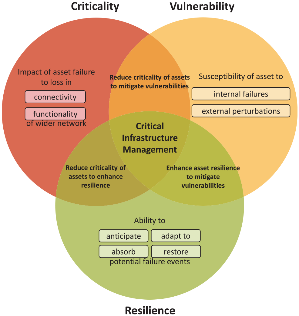
Conceptual distinction between criticality and related concepts.
Current Methods in Assessing Criticality and Failure Propagation
There is an increased research interest in assessing asset criticality and understanding failure propagation, using network-based approaches. These approaches focus on topological and flow-based metrics ( 2 , 19 ). Topological metrics evaluate the internal connectivity of an asset to other assets, based on their representation as nodes in a network using network theory (e.g., degree and betweenness centrality measures). Node degree refers to the number of links from the node; betweenness centrality refers to the fraction of shortest paths between an origin–destination pair whereby resources flow through the node, summed across all origin–destination pairs ( 20 ). On the other hand, flow-based metrics evaluate assets based on their real-world functionality in the supply of essential goods, services or utilities to the urban population (e.g., usage demand, flow capacities and resource transportation times) ( 10 ).
Several related research studies focus on asset criticality evaluation and failure propagation in transportation networks. Rodríguez-Núñez and García-Palomares ( 17 ) utilized flow-based metrics when simulating link closures between adjacent stations arising from targeted attacks; if an alternative route between them exists the increase in travel time between them is evaluated, and if no such route exists the number the unfulfilled passenger trips is determined. Faramondi et al. ( 20 ) identified that trade-offs can exist between centrality and passenger flow measures, and thus formulated a weighted combination of these metrics to analyze station criticality within the Central London Tube. A similar approach was undertaken by Zhang et al. ( 21 ), combining metrics from the node-place-design model (i.e., public transportation connectivity, pedestrian accessibility and surrounding land usage) using principal component analysis. Hadjidemetriou et al. ( 22 , 23 ) combined closeness vitality measures and observed daily traffic flows to develop a hybrid criticality index for maintenance prioritization of road bridges over their lifecycle. Liu et al. ( 24 ) simulated a variety of random failures and targeted attacks, such as sequentially attacking stations of the highest passenger loads or centrality metrics, on railway networks in the Chengdu-Chongqing region, China. They then analyzed both topology- and flow-based failure cascades from excessive station demand as passenger flows are rerouted.
For electricity networks, Yang et al. ( 25 ) modeled the rerouting of flows and rescaling of energy generation (frequency control) and consumption (load shedding) to illustrate failure propagation within the North American transmission grid in the event of successive cable failures. Models were also proposed by Nie et al. ( 26 ) for stochastic failures and recovery of transmission lines (links) from load-shedding and redistribution operations.
There are a few studies that focus on utilizing multilayer networks to model similar infrastructure networks, such as in intermodal transportation ( 27 ) and in interconnected electricity grids owned by different operators ( 28 ). However, multilayer networks are also particularly suited to analyzing failure propagation across distinct infrastructure systems. They allow for greater tractability and data transparency in modeling different resources and infrastructural asset types. Furthermore, they support the modeling of interdependencies between assets of different infrastructure systems as compared with conventional single-layer networks ( 29 ). Goldbeck et al. ( 30 ) segmented London’s rail and electricity networks further into individual network layers, modeling the provided services (e.g., passenger flow, electricity distribution). The asset layers detailed relationships between components (e.g., signal controls, rail tracks). A similar flow-based study was conducted by Lee II et al. ( 31 ) covering post-failure restoration of electricity, transportation and telecommunications networks in New York. Thacker et al. ( 32 ) developed a criticality metric focusing on the number of users directly or indirectly affected by failures, based on population census data and infrastructure demand data, and applied it across many networks including transportation, utilities and telecommunications in England and Wales.
In summary, there is no established comprehensive method for simulating the dynamics of city-wide critical infrastructure within a multilayer network using real-life data, even though this is crucial in capturing a realistic higher-order representation of failure propagation. Having this research gap in mind, the current paper aims to propose a methodology for modeling infrastructure in large-scale city environments and their failure propagation dynamics as complex networks, from which the criticality of infrastructural assets can be assessed and cross-compared. The modeling methodology makes several novel contributions to existing literature by modeling the dynamics of rerouted resource flows in the event of asset failures and combining load-based failures with failure diffusion processes. Furthermore, two criticality metrics, normalized topological impact (NTI) and normalized economic impact (NEI), are proposed to measure the topological extent of infrastructural failures and economic impacts resulting from the failure propagation of given initial failure scenarios. This methodology is applied to a representative case study of the exposure of rail transportation network to failures in electricity network in London, UK.
Methodology
Infrastructure Modeling Methodology
Urban infrastructure in general is represented as a multilayer network, with the layers demonstrating individual infrastructure networks being studied. The assets are represented as nodes which are involved in the supply, storage and consumption of resources, or links which are involved in the transportation or movement of these resources. For example, as illustrated in Figure 2, power generators, substations, loads and train stations are represented as nodes, and power cables and rail connections as links. Figure 3 outlines the key phases in the modeling of this multilayer network.
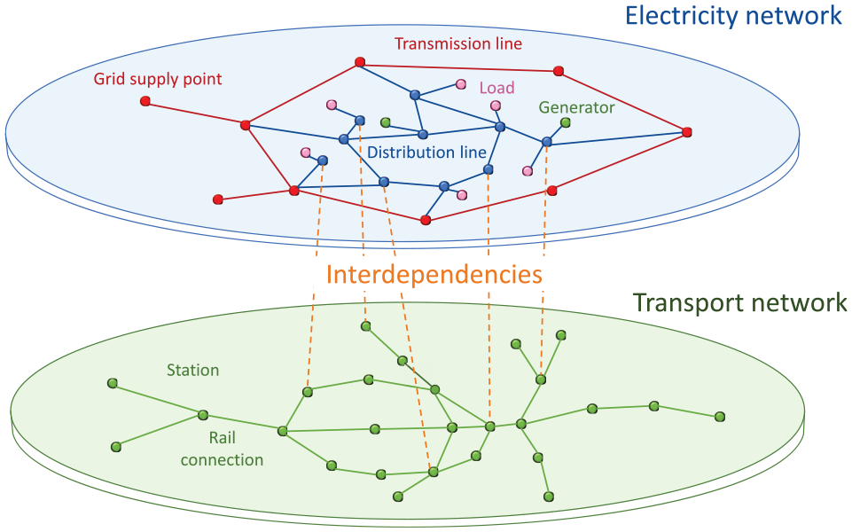
Illustrative example of multilayer infrastructure network.
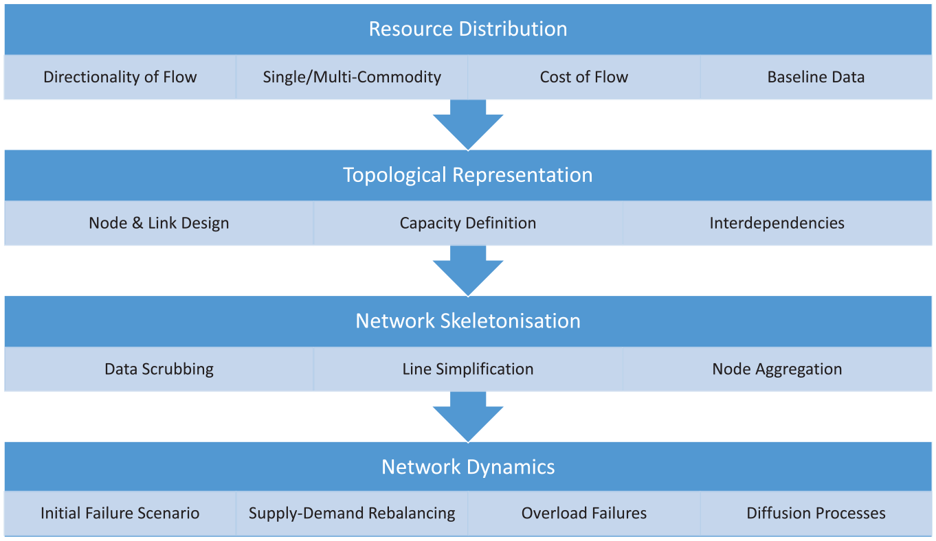
Overall modeling framework for interdependent urban infrastructure.
The first phase involves modeling the distribution of resources across various types of infrastructure networks. It is important to distinguish between multi-commodity networks (with a requirement for specific resources to flow between specific origin–destination pairs to fulfill demand, such as rail transportation), and single-commodity networks (with no such specific requirement, such as electricity distribution) ( 30 , 31 ). It should also be identified whether resource flows follow a minimum cost flow (e.g., rail transportation) or a random path (e.g., electricity distribution) ( 33 ).
The next phase focuses on the representation of various assets as nodes and links, a process described in Herrera et al. ( 34 ). The represented network topology can be thereafter simplified to reduce computational complexity when simulating failure propagation, especially for infrastructure in large metropolitan areas. This is known as network skeletonization and has been applied in various infrastructure networks. One approach is to combine nodes based on their geographical location and characteristics, such as in the multiscale decomposition of water distribution networks defined by district metered areas (DMAs) ( 35 ). Other works focus on metric-based approaches to evaluate the graph-theoretical representation of skeletonized networks, such as by augmenting the adjacency matrix of U.S. air transportation networks ( 36 ).
The final phase is modeling the network dynamics as failures are propagated. First, an initial failure is introduced into the network, and the resource flows within the network are recomputed. Thereafter, two main modes of propagation are considered: load-based failures arising from flow redistribution and propagation of physical failures represented by stochastic diffusion processes between a failed node and its adjacent nodes exposed to this failure. These capture the real-life effects of cascading and common-cause failures. Figure 4 illustrates the failure propagation dynamics, assumed to be an iterative process over a time horizon beginning from an initial failure. This approach was adapted from Chen et al. ( 37 ) and Korkali et al. ( 38 ) which proposed a computational sequence for cascading failures across interdependent telecommunications and electricity networks. In this work a similar approach is undertaken.
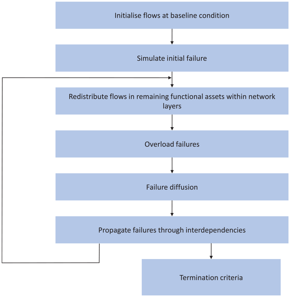
Computational sequence for failure propagation.
Multilayer Network Representation
Mathematical Nomenclature
The mathematical representation proposed here is largely adapted from Boccaletti et al. (
29
) and Goldbeck et al. (
30
). Let
Each link
An ordered tuple of its start and end nodes
maximum flow capacity,
resource flow,
a state variable indicating the functionality of the link,
Each node
maximum throughput capacity,
imported/exported flow that enters/exits the network via n,
amount of resources generated and consumed at n,
total resource throughput across n,
functionality,
For each pair of nodes
Each dependency
an ordered tuple of its start and end nodes
a state variable indicating the functionality of the dependency at time t,
Baseline Initialization
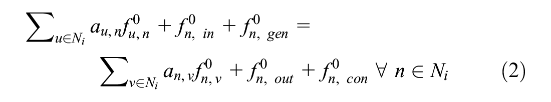
The initialization of resource flows at a predefined baseline condition depends on the type of network. For multi-commodity networks, the flow

For single-commodity networks, the total resource inflows and generation equals resource outflows and consumption for all nodes in the whole network. This is equivalent to solving:
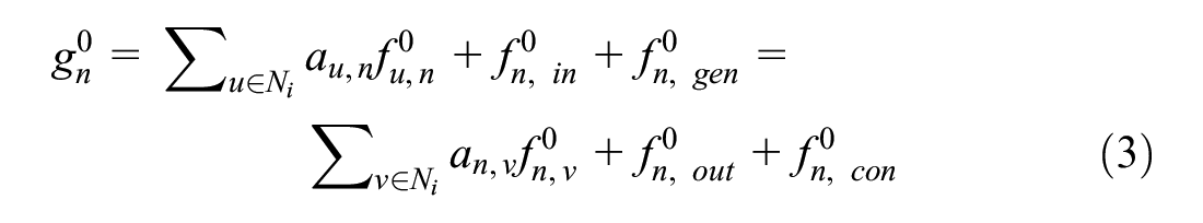
The resource throughputs across each node
Failure Propagation Dynamics
As more nodes and/or links fail over successive iterations t, the evolution of
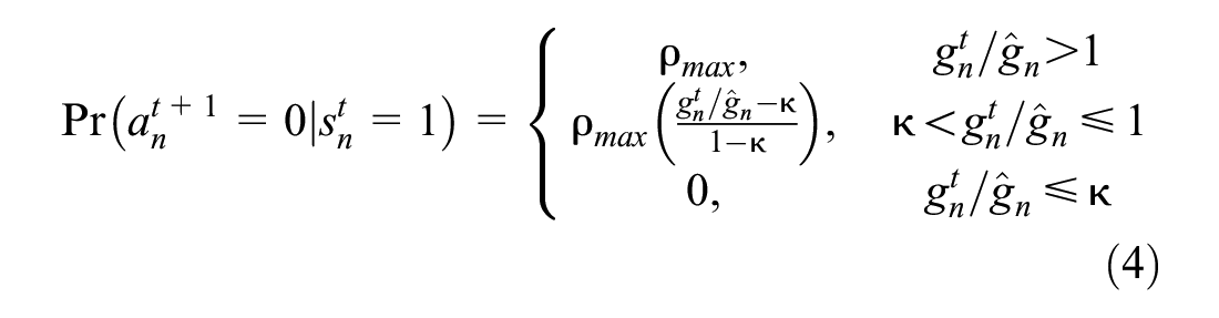
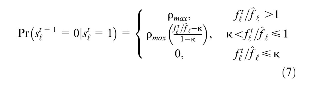
At each iteration, load-based failures are modeled as such: each node n fails stochastically, if the total throughput across n is close to or exceeds its available holding capacity at time t. A piecewise linear model (Equation 4) is adapted from Nie et al. ( 26 ), based on the logic that the risk of asset failure increases with increasing asset utilization toward its capacity:
where

where
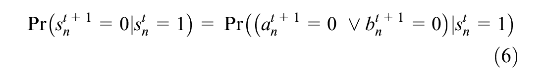
The failures of links are similarly modeled, but only considering load-based failures:
Physical interdependencies are represented as links between two nodes from two different layers defined based on real-life data. If a node in one layer fails, all its connecting interdependencies fail at the same time, and in turn the node at the other end fails with a probability proportional to the fraction of its own physical interdependencies failing. For geographical interdependencies, if a node in one layer fails, all nodes in the other layers within a certain distance threshold
Asset Criticality Definition
A combination of topological metrics from complex network theory, as well as flow-based metrics, is utilized to quantify and compare the criticality of assets within the same multilayer network. From prior literature, a conventional measure of a node’s criticality is typically determined by looking at capacity, resource flows and various centrality measures of nodes in the original network (
20
). However, to capture the impact of higher-order failure propagation over time, two time-based criticality metrics, NTI and NEI, are proposed. Their time-based nature is useful for policymakers and asset owners to evaluate infrastructure networks at any time snapshot over a failure propagation time horizon, from the time of an initial failure until the time of intervention in the form of repair and maintenance. Additionally, the normalization of metrics also supports cross-comparison between different or heterogeneous types of assets. A larger value of NTI and NEI at a defined time
From a network topological-based perspective, the normalized topological robustness (NTR) at time
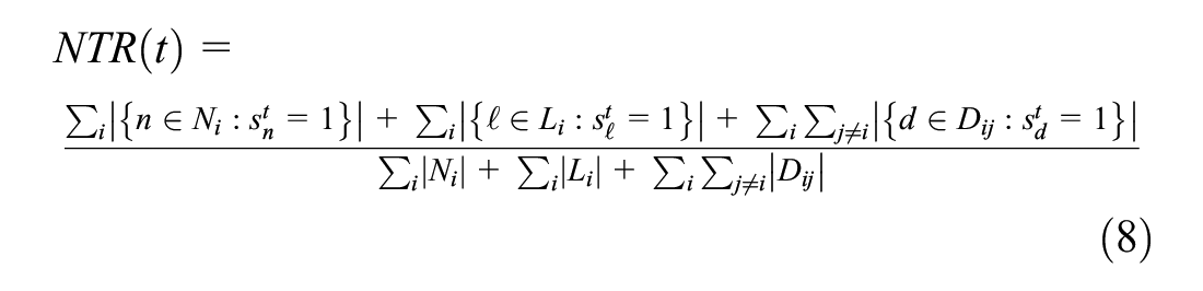
The NTR metric proposed here is a generalization of the robustness metrics used in Liu et al. (
24
), with the key improvement being that this also considers all connected subnetworks that remain functional, and not just the largest subnetwork (i.e., the “giant connected component”). Furthermore, Zeng and Liu (
39
) noted the importance of incorporating functional links into network robustness metrics, especially for infrastructure networks whereby link-based failures also occur. With this, the complementary term

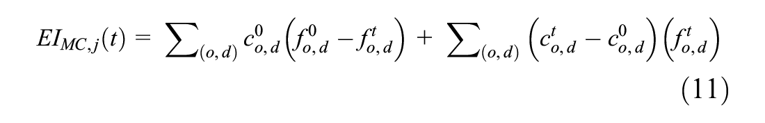
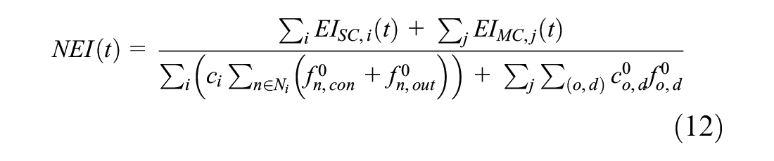
From a flow-based perspective, a classical approach for an individual infrastructure network would be to consider the fraction of resource demand that can still be fulfilled at time t > 0 ( 13 ). In the context of a multilayer network with several resource types, the NEI of the failure propagation over time is proposed to allow for comparative analysis of different resource prices and economic costs across different infrastructure networks. This approach is as opposed to considering the fraction of nodes and links within the network that remain functional, because quantifying the failures of topological features does not always reflect the economic impact of failure propagation.
For each single-commodity network i, the economic impact
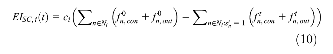
where
where
Case Study
Location and Infrastructure Selection
The methodology described above was applied to the rail and electricity infrastructure networks of Greater London, UK. This location and these networks were selected because of the general availability of data and because they allow for a representative application of the proposed modeling methodology to a large-scale urban metropolitan area. Furthermore, it was identified that electricity networks have become significant contributors to interdependencies with other physical infrastructure ( 40 ), which this study examines. For example, power outages can affect the electrification of rail transportation and stations, and on the other hand, increased train frequencies with higher rail demand can lead to higher electrification demand. The baseline conditions for the case study were selected such that train and electricity demand are the highest based on the datasets’ available time granularity. This corresponds to the morning peak period (0700–1000 h) for train demand averaged across the entire 2019 year, and 2019 winter season for electricity demand.
The rail network layer was modeled as a directed multi-commodity network, with resource flows being the number of passenger trips per hour, and with train stations and the rail connections modeled as nodes and links respectively. Train stations and tracks from the London Underground, London Overground, Transport for London (TfL) Rail (including Crossrail, renamed the Elizabeth Line in 2022) and the Docklands Light Railway lines were considered. Information about the train stations and lines was obtained by merging the London Multiplex Transport dataset ( 41 ) with the TfL Rolling Origin & Destination Survey (RODS) dataset ( 42 ). The TfL RODS dataset includes trip durations between adjacent pairs of stations, as well as the origin–destination matrix of all pairs of rail stations. This allows passenger flows to be computed both at baseline conditions and when trips need be rerouted during failures. The capacity of each rail connection was defined as the number of trains along the link ( 43 ), multiplied by the seating and standing capacities of the rolling stock currently in use ( 42 , 44 , 45 ).
The passenger flows in the rail network were calculated using the TfL origin–destination matrix ( 42 ) as described in Equation 1, assuming that passengers will always take the shortest path between each origin–destination pair by travel time. During failure propagation, passenger trips are rerouted if there is a new link failure along affected origin–destination paths, otherwise they become unfulfilled if no origin–destination path exists anymore. Furthermore, when a rail connection is already at capacity, any excess passenger trips will become unfulfilled.
The electricity network layer was modeled as a directed single-commodity network, with the resource flows being electrical power. The full electricity chain from generation, high-voltage (400 kV–275 kV) transmission, medium-to-low-voltage (132 kV–11 kV) distribution to consumption was considered. Modeling this requires the triangulation of three major databases. The UK Power Networks (UKPN) Long-Term Development Statement (LTDS) ( 46 ) contains information for the Greater London distribution grid, distributed generation, overhead lines and underground cable tunnels, substations and transformers to step up/down electrical voltages, and electricity loads aggregated at the substation level. Operating voltages, circuit capacities, generation and load data are also included. This technical dataset is not publicly accessible and was requested and acquired from UKPN. The National Grid dataset ( 47 ) was used to identify the transmission cables and substations immediately encircling the Greater London boundary and the distribution grid, such that a single contiguous electricity network could be modeled. The OpenStreetMap (OSM) database ( 48 ) was also referenced to identify any substations and electrical lines that are used for rail traction purposes, but did not appear in both UKPN LTDS and National Grid datasets. Electricity exports out of Greater London were not considered. The overhead lines, underground cables and transformers were modeled as links, while generators, substations and loads were modeled as heterogeneous nodes.
The edge current flow betweenness method ( 33 ) is used to model electricity flows, from the generators and transmission grid supply points (GSPs) where electricity enters the network, to the loads where electricity is consumed. As failures propagate within the electricity grid, when electricity demand exceeds supply for any subnetwork, the loads at substations within that subnetwork will be selected to fail successively at random until demand can be met, so as to mimic load-shedding operations by grid operators.
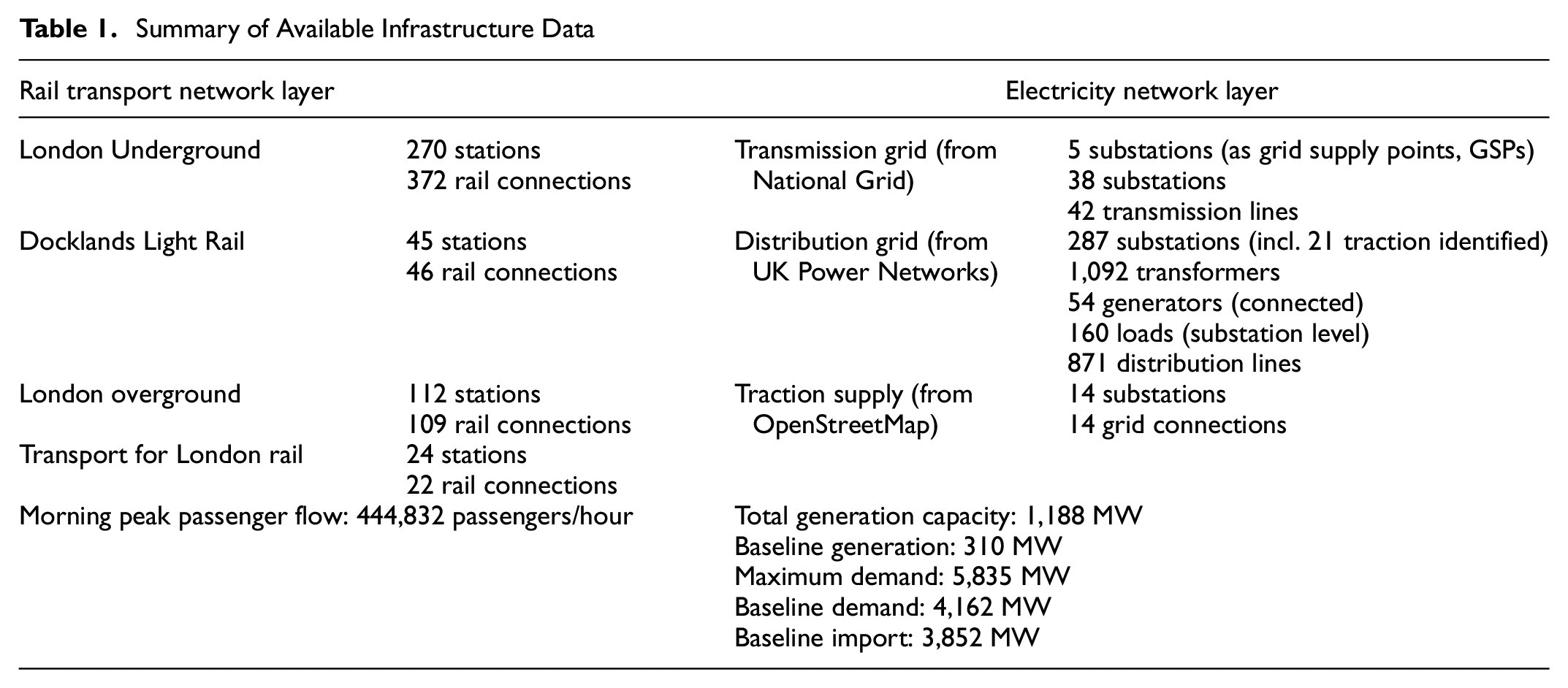
The coordinates for infrastructural assets were geocoded using the QGIS geographic information system ( 49 ) and OSM database ( 48 ). Table 1 summarizes the data available.
Summary of Available Infrastructure Data
Physical interdependencies were created by identifying all traction substations from the triangulation of various datasets, and then connecting them to the closest node in the rail network layer. The electrical loads required for train traction were estimated from TfL’s energy purchasing reports (
50
). For geographical interdependencies, the distance threshold
The modeled multilayer network was simplified through a combination of data scrubbing, line simplification and node aggregation. Nodes and flow properties were aggregated in the rail network layer: by (a) combining interchange stations spread out across multiple sites (e.g., Bank and Monument) based on the Standard Tube Map’s definition ( 51 ), and (b) combining adjacent non-interchanging stations into a single hypernode. For the electricity network layer, transformers located within the same substation location were aggregated into the same substation hypernode, such that each hypernode represents a combination of location and operating voltage. This thus significantly preserves the topology of the multilayer network; for instance, all rail connections to and from interchange stations are preserved, and the locations and connections between electricity substations are preserved. The abovementioned network skeletonization led to a 49.8% reduction in nodes and 28.6% reduction in links. The final three-dimensional representation of the modeled networks is presented in Figure 5.
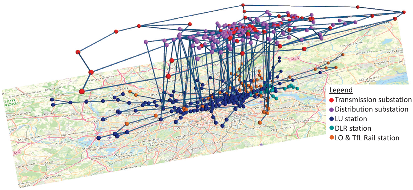
Three-dimensional representation of multilayer network with interdependencies.
Criticality Assessment
For criticality assessment, the NTI metric was calculated for the modeled multilayer network using Equations 8 and 9 as explained above. The NEI is calculated based on in Equations 10 to 12, and this is contributed by: (i) unfulfilled train passenger trips caused by rail closures, (ii) increases in travel time for rerouted passenger trips given train disruptions, and (iii) unfulfilled electricity demand from grid failures. The economic impacts from the rail and electricity networks can thus be respectively rewritten as Equations 13 to 14:
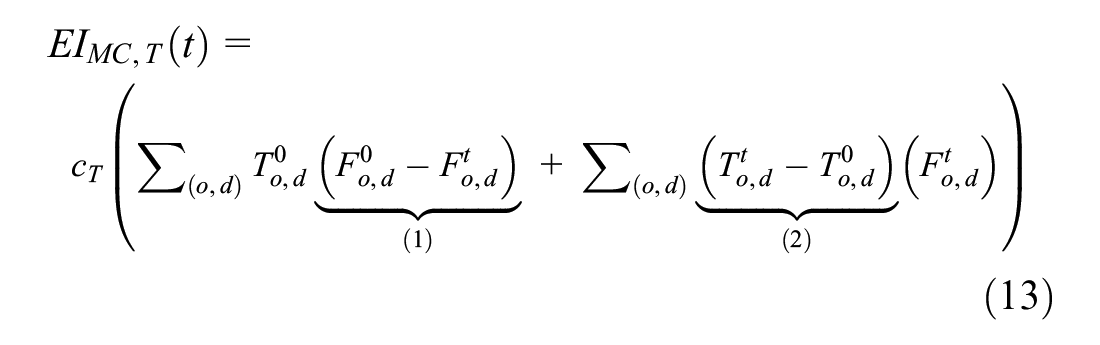
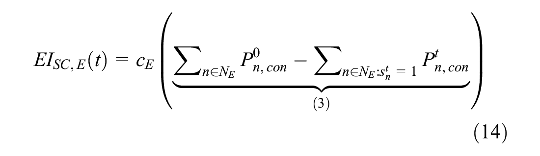
where t is time,
Implementation in Python
The multilayer network structure was created in Python 3 using the networkx library ( 54 ). networkx also contains several algorithms utilized in this work: Dijkstra’s algorithm to calculate shortest paths for the rail network, current flow betweenness calculation for the electricity network layer, connected subgraphs detection and centrality calculations. The simulations were conducted on the Distributed Information and Automation Laboratory server at the University of Cambridge with specifications as follows: Intel Xeon CPU E5-2680 v4, 2.40 GHz, 64 GB RAM. The processing time for each simulation was 40 min per 30 iterations of failure propagation dynamics as described in Figure 4. The Python code is available on a GitHub code repository, https://github.com/weepctxb/iCASCADE, on request.
Results and Discussion
Base Case Simulation
The developed model was preliminarily validated by considering a base case scenario, which is an initial failure of the largest power station in Greater London (Enfield Power Station). The multilayer network is then subjected to the failure propagation dynamics as illustrated in Figure 4, over a discretized time horizon with each time step corresponding to one iteration of the failure propagation. The units for simulation timescale would be in the order of magnitude of minutes, corresponding to what is observed for electricity and rail network failures in real life (
6
). The tunable parameters
Eight replication runs (Figure 6) were conducted to ensure replicability of results, with each simulation terminating early if the network had completely collapsed or if there was no further failure propagation for consecutive time steps. The average time for NTI to approach 0.5 was measured to set a benchmark time
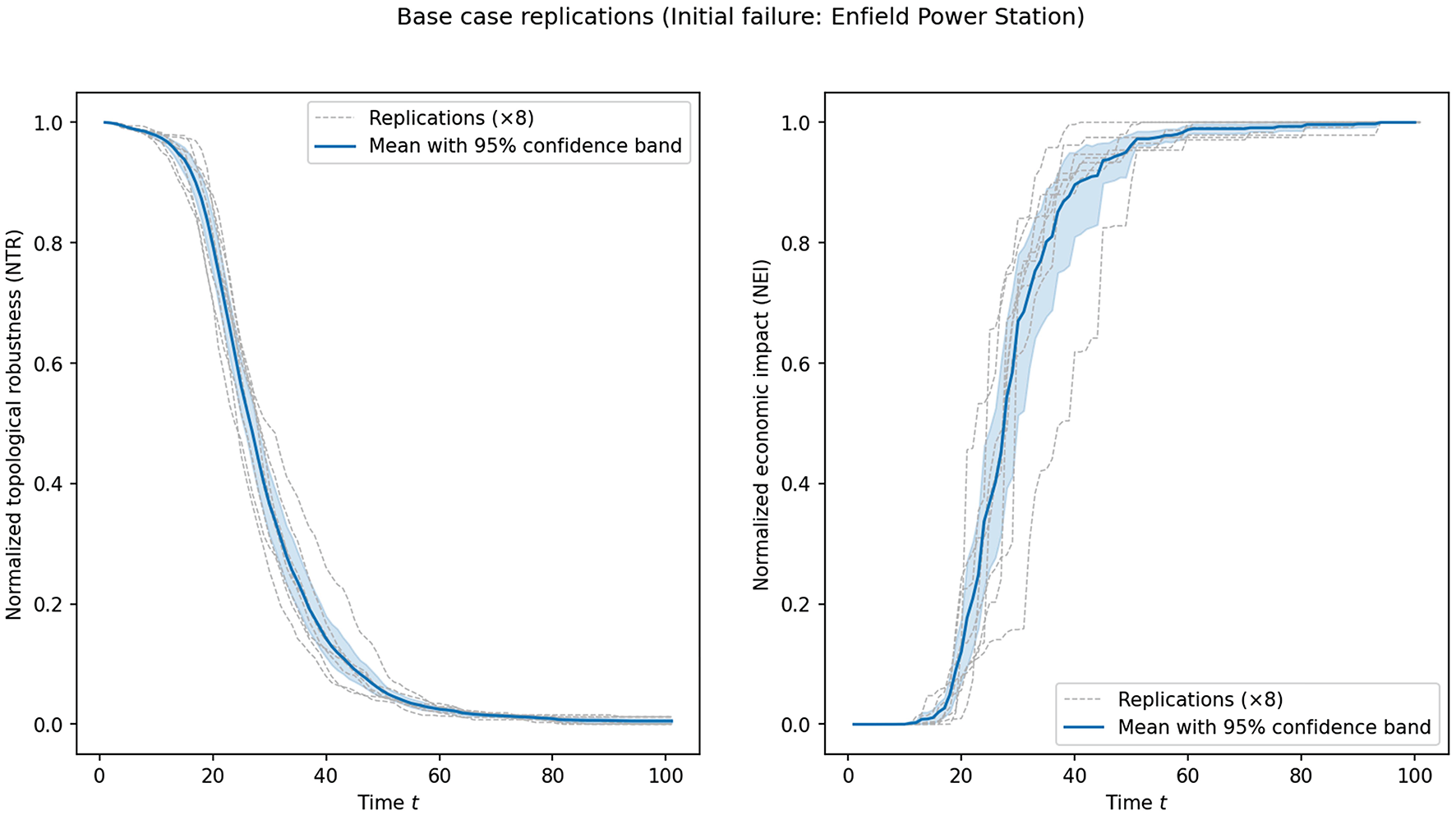
Base case simulation of (a) normalized topological robustness (NTR) and (b) normalized economic impact (NEI) over time (Enfield Power Station).
Figure 7 visualizes the failure propagation over 30 time steps for one of these replications, with green indicating functional nodes and links, and red indicating nodes and links that have failed at that time step. It can be seen that with an initial failure of Enfield Power Station, apart from the diffusion of the failures across adjacent assets, there are shortfalls in electricity supply resulting in load-shedding operations and thus isolated load disconnection failures at substations as mimicked in the failure propagation dynamics. At the same time, power failures can affect train stations via electrical substations, thus leading to the rerouting of passenger flows which causes further stress on the rail network layer.
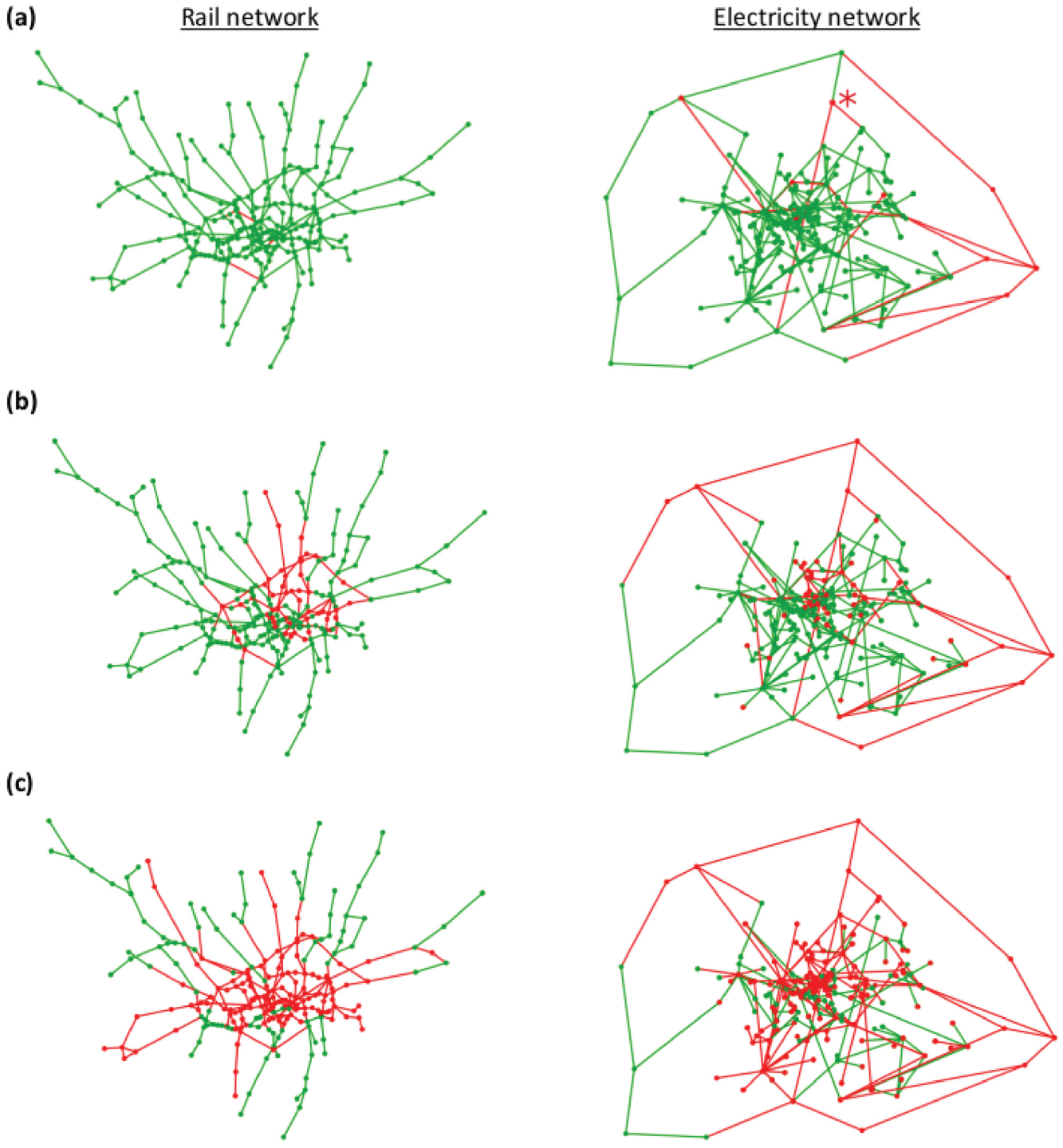
Visualization of failure propagation of rail network (left) and electricity network (right) over 30 iterations: (a) t = 10, (b) t = 20, and (c) t = 30.
Comparative Criticality Analysis
To demonstrate the criticality comparison of various assets within the multilayer network, a preliminary shortlisting of train stations to analyze was conducted. Because of large computational complexities, it was not possible to conduct simulations for all possible initial failures at all train stations in the multilayer network. Instead, the most prominent train stations were shortlisted based on their attributes of interest (AOI), as shown in Table 2, namely: node degree, betweenness centrality, hourly station capacity and baseline hourly passenger throughput. These attributes were selected based on the various asset attack strategies categorized by Liu et al. (
24
) (i.e., high load, node and betweenness attacks). For each shortlisted station, several replications of simulations based on its initial failure are run over the time horizon
Shortlisted Train Stations for Analysis, With Attributes of Interest (AOI), Normalized Topological Impact (NTI) and Normalized Economic Impact (NEI) Rankings (for each ranking, the top 10 stations are in bold)
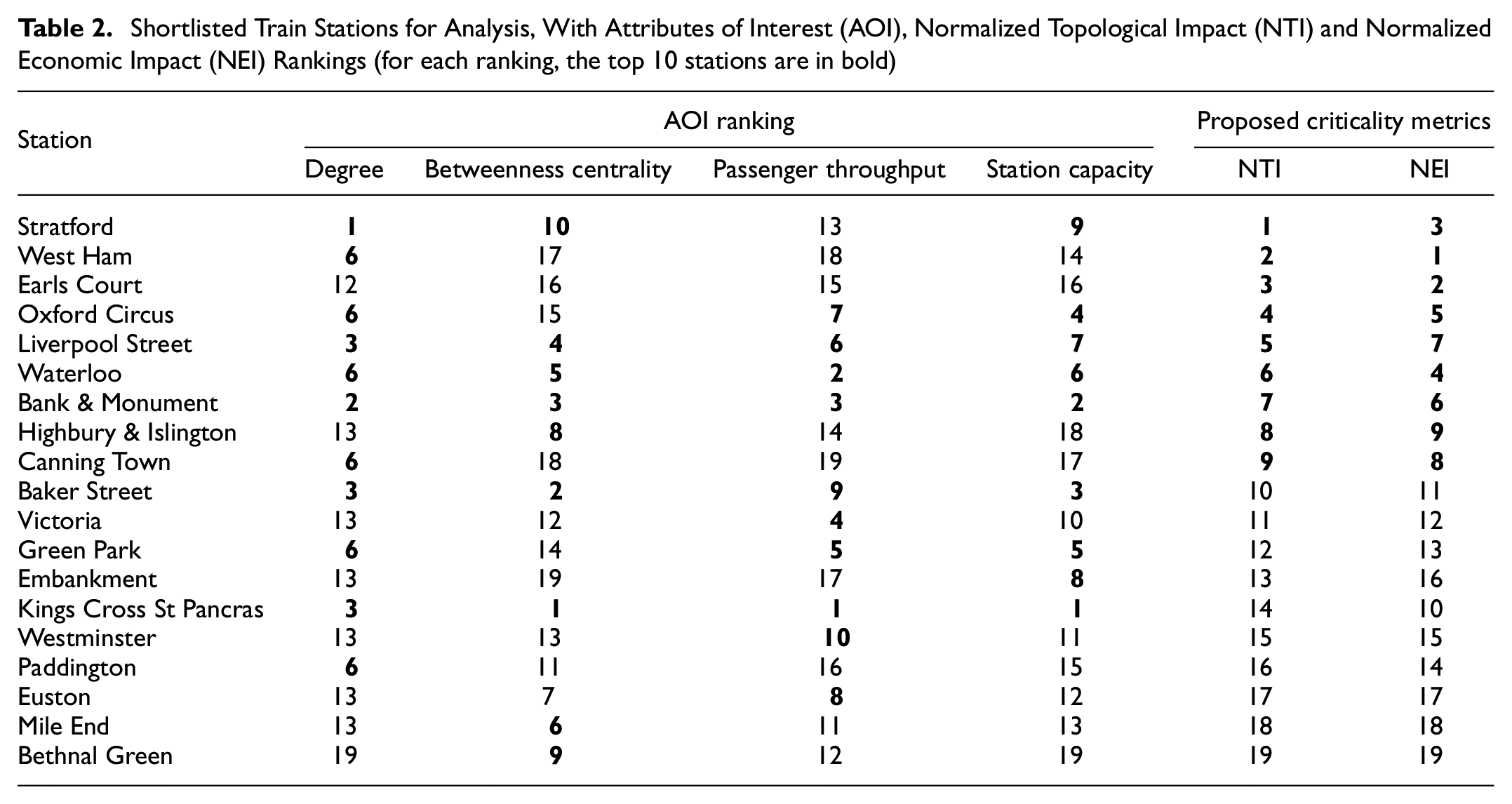
The rankings in NTI, NEI and attributes of interest (AOI) were further investigated in the pairwise scatterplot analysis in Figure 8, in which each individual scatterplot and parameter distribution is indicated by the labels in both horizontal and vertical axes. The betweenness and passenger throughput AOIs were omitted to reduce visual complexity because of their high collinearity with station capacity. As expected, the degrees of train stations are positively correlated with their throughput capacities, because these correspond to the larger interchanges within the rail network with much higher passenger volumes. However, there are not always clear correlations between the AOIs when compared with NTI or NEI. A notable example is that although Kings Cross St Pancras is ranked highest for betweenness, passenger throughput and capacity, it ranked 14th and 10th for NTI and NEI respectively (Table 2). This can be explained by the number of different rail lines surrounding its location in central London, implying that passenger flows can be easily rerouted by several alternative routes in the event of failure.
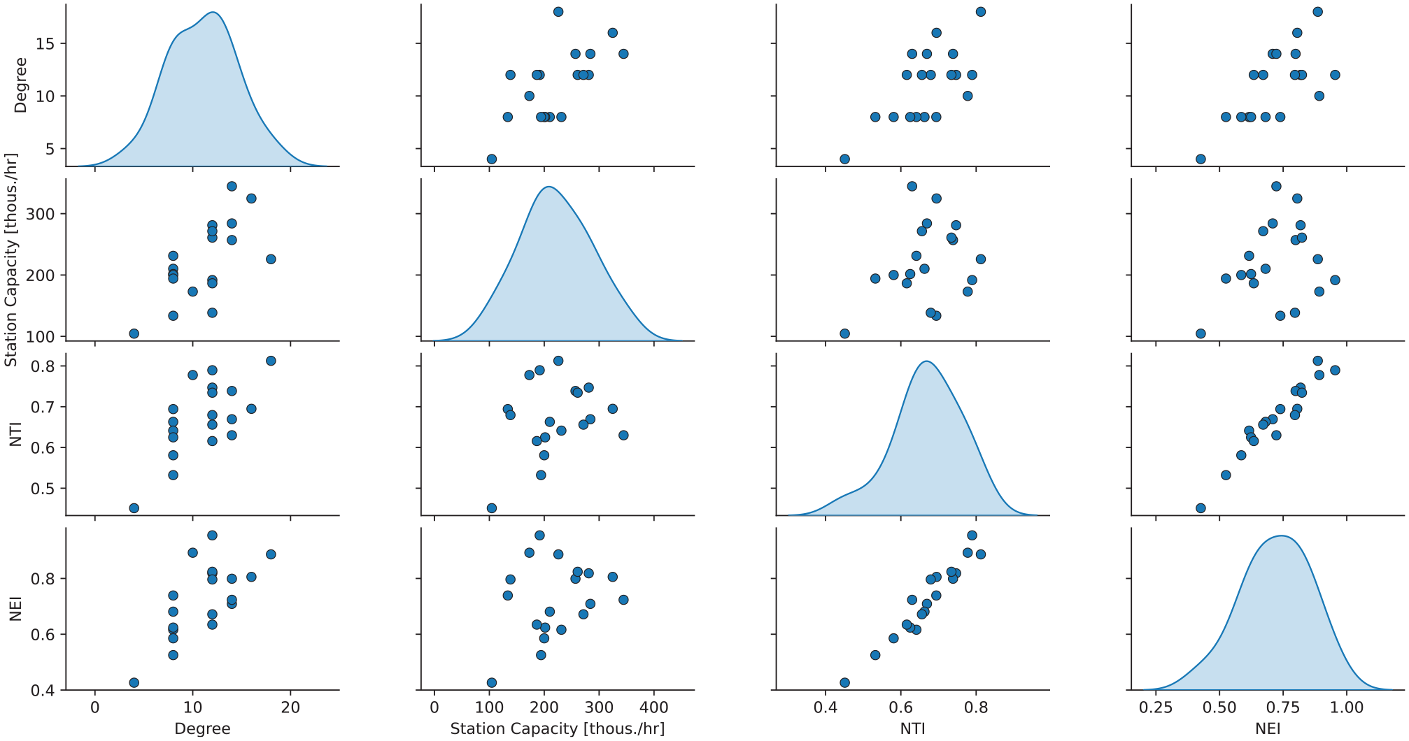
Pairwise scatterplots of shortlisted train stations by attributes of interest (AOI), normalized topological impact (NTI) and normalized economic impact (NEI).
Conversely, Stratford is ranked first and third for NTI and NEI respectively, even though it is ranked much lower in betweenness, passenger throughput and capacity, because of its many rail connections, as explained by its highest node degree. A node failure at Stratford would lead to a segmentation of the rail network layer into multiple subnetworks, disconnecting line segments which contribute to unfulfilled passenger trips between eastern and central London. This is similarly the case for West Ham, ranked second and first for NTI and NEI respectively, being a major interchange connecting with rail lines that branch toward the east of London. Although AOIs measured at baseline conditions serve as a good initial heuristic for identifying and prioritizing critical assets, they are not always representative in capturing the influence of higher-order failure propagation on the infrastructure network.
Focusing on the scatterplot between NTI and NEI (Figure 9), both metrics are generally closely correlated, which is intuitive because greater extent of infrastructure failures should be associated with greater economic costs. However, this correlation is not always linear and notable deviations exist, which also result in different rankings when assets are ranked by their NTI or NEI. This emphasizes that topological robustness of infrastructure networks does not always reflect the resulting economic impacts of infrastructural failures. Therefore, topological metrics such as the proposed NTI metric should be complemented by other flow-based metrics such as the proposed NEI metric, to provide a more representative and holistic assessment of the potential consequences of infrastructural failures.
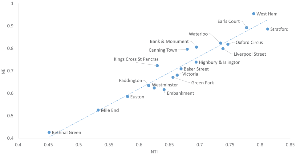
Normalized topological impact (NTI) versus normalized economic impact (NEI) for shortlisted train stations.
Conclusion
This paper presents a methodology for modeling heterogeneous infrastructural assets within a large-scale city environment, addressing present challenges in modeling infrastructural assets utilizing available real-life data. The research contribution can be summarized by the multilayer network representation of infrastructure, the simulation of failure propagation dynamics and the time-based NTI and NEI criticality metrics. Specifically, this methodology incorporates network skeletonization methods to reduce computational complexities especially for multilayer infrastructure networks covering larger metropolitan areas. Furthermore, combining load-based failures with failure diffusion processes provides a more realistic simulation of failure propagation scenarios. Lastly, the time-based NTI and NEI metrics allow for the criticality assessment of infrastructural assets, by considering higher-order impacts of asset failures, over a time period whereby asset failures are propagated till the point of intervention by asset owners.
The model can assist infrastructure asset owners in simulating a wide range of scenarios to compare the criticality of assets. Utilizing the case study’s infrastructure network as an example, failures in power generation can lead to suspensions of train services or inoperability of train stations, and this can result in additional strains on the overall rail network arising from excessive station demands as passenger flows are rerouted. This can be modeled by defining and varying the power station in question to fail initially and conducting multiple simulations. Beyond this case study, the methodology can also be transferred to other types of infrastructure networks (such as telecommunications or other public transportation modes), since the modeling framework is generalizable to accommodate any number of single-commodity or multi-commodity networks with assets being modeled as either nodes or links depending on the application context. Additionally, as there are trade-offs between the reduction of node and link features and resulting data accuracy because of network skeletonization, more robust approaches identified in the literature can be employed as a future research direction to evaluate the skeletonization of even larger multilayer networks.
With this, asset owners can also adopt this model to identify and evaluate potential measures to mitigate the criticality of various assets. Operations and maintenance-related measures are evaluated over shorter timespans, while design-related measures are primarily concerned with longer-term criticality analysis in which the topology of interdependent infrastructure networks is evaluated. These include adding new links and/or nodes around prioritized critical assets, increasing the coupling of physical and cyber interdependencies to buffer against failure propagation across network layers, and enhancing the physical capacity of susceptible nodes and links with the highest simulated occurrence rates of load-based failures.
The presented work faces some limitations that further works in progress aim to overcome. The synchronization of the timescales of load-based failures and failure diffusion across infrastructure networks were assumed to be the same and can be refined further. This involves determining appropriate time step intervals for both mechanisms across both networks, which were assumed to be similar and corresponding to one iteration of the modeled failure propagation dynamics, to improve the accuracy of dynamic simulations. This is also closely related to the calibration of the model parameters
Another simplifying assumption that can be investigated was that rail passengers follow the path of shortest traveling time. This may not always hold true, especially for longer-distance trips across the Greater London area, as these may also be influenced by other factors such as waiting times and train frequencies. An alternative method would be to utilize a hybrid combination of random walks and shortest path considerations. Furthermore, there are several opportunities to increase the level of detail in this proposed model to improve the realism of the infrastructure networks. These include: incorporating the dynamics of asset recovery strategies (e.g., repair and maintenance), so that network perturbations such as partial asset failure states can be modeled, and relaxing the assumption that the demand and supply of resources are static throughout the time horizon. It is anticipated that future developments in the identified research directions will facilitate a more extensible modeling of cascading failure propagation and criticality assessment for infrastructural assets, to strengthen existing protection and failure mitigation measures by infrastructural asset owners.
Footnotes
Acknowledgements
The authors would like to acknowledge UK Power Networks for providing their Long-Term Development Statement’s datasets for this research.
Author Contributions
The authors confirm contribution to the paper as follows: study conception and design: X. B. Wee, M. Herrera, G. M. Hadjimetriou, A. K. Parlikad; data collection: X. B. Wee, M. Herrera, G. M. Hadjimetriou; analysis and interpretation of results: X. B. Wee, M. Herrera, G. M. Hadjimetriou; draft manuscript preparation: X. B. Wee, G. M. Hadjimetriou, M. Herrera, A. K. Parlikad. All authors reviewed the results and approved the final version of the manuscript.
Declaration of Conflicting Interests
The author(s) declared no potential conflicts of interest with respect to the research, authorship, and/or publication of this article.
Funding
The author(s) disclosed receipt of the following financial support for the research, authorship, and/or publication of this article: This work was supported by the European Community’s H2020 Programme MG7-1-2017 Resilience to Extreme (Natural and Man-made) Events, under Grant no. 769255, “GIS-based infrastructure management system for optimized response to extreme events of terrestrial transport networks (SAFEWAY)”.