
Abstract
Exclusive bus lane (EBL) is one of the most common transit prioritization strategies implemented to improve transit speed. However, one major drawback of implementing EBLs is the associated reduction in road capacity left for other road users. In corridors with EBLs and infrequent bus service, the lanes are underutilized for extended periods of time. Dynamic bus lane (DBL), a new priority strategy enabled by vehicle connectivity, can provide buses with priority while allowing the general traffic to access the bus lane when buses are not present. Although the DBL concept is promising, a limited number of studies have explored its effectiveness under various conditions. Thus, this paper investigates the impacts of DBLs through a comparison with EBLs and mixed traffic operation under different levels of traffic demand and transit frequency. As a case study, the Eglinton East corridor in Toronto, Canada, was simulated using Aimsun Next, and different scenarios of behavioral impacts were considered in the analysis. The results reveal that DBL is a promising strategy with potential to improve the overall corridor performance over a wide range of traffic and transit service conditions, especially under intermediate traffic demand levels. On the other hand, EBL can be an efficient prioritization strategy that improves the overall corridor performance under high traffic demand and high transit frequency levels, but only if accompanied by a major mode shift from auto to transit.
Keywords
The demand for mobility is on the rise in every city around the world. This increase is bound to exacerbate the levels of congestion, noise, greenhouse gas emissions, and traffic accidents. Thus, improving the efficiency and attractiveness of public transit service has been frequently proposed as the sustainable solution to reduce traffic congestion and its adverse impacts in urban areas. Exclusive bus lane (EBL) is one of the most common transit prioritization strategies that improve transit speed and offer high-quality transit service ( 1 , 2 ). However, the major issue for the EBL strategy is the significant reduction in the road capacity for other road users, which increases traffic delays and queues ( 3 , 4 ). Such negative impact on traffic is often justified by system operators in the hope that it will induce mode shift to transit. However, if the enhanced transit performance does not induce a significant mode shift from driving to transit, the net effect of an EBL on all users in total person delay can be negative. Additionally, if bus service frequency is relatively low, this will result in long gaps during which the EBL is not used. To address this issue, intermittent bus lanes (IBLs) were proposed by Viegas and Lu ( 5 ). IBLs were originally proposed to complement transit signal priority. This type of lane was designed with the following operating concept: vehicles ahead of a bus but sharing the same lane should either stay in the lane or move over to the adjacent lanes; simultaneously, vehicles traveling in the adjacent lanes cannot move over to the bus lane as long as there is a bus occupying it. Subsequently, a variation of this concept was proposed, whereby the general traffic is forced to leave the bus lane and move over to the adjacent lanes if a bus is traveling in the lane ( 6 ). In general, IBLs allow private vehicles to use transit lanes when transit is not present ( 6 , 7 ). IBL is considered as an innovative solution that improves transit service performance while promoting the efficient usage of road capacity. In general, IBLs were proposed using variable message signs (VMS) and longitudinal stud lights that are embedded in the pavement of the road to inform the drivers of the status of the lane and whether they can use it or not ( 8 ). Early studies on IBLs focused on section-based IBLs which use VMS to clear the entire section on the arrival of a bus ( 9 – 14 ). In this case, cars cannot use the lane until the bus clears the last VMS at the downstream end of the section. However, this type of IBL may bring some disadvantages. For example, long sections of IBL may deteriorate the performance of the general traffic, similar to the EBL ( 8 ). Additionally, the variability of the lengths of the road sections may cause asymmetric benefits of the IBL. Thus, the original IBL concept was recently modified to allow the general traffic to use the lane behind the bus (after the bus has passed) and prioritize transit in a predetermined length ahead of the bus. This length, called the “clear distance,” defines the protected road section which the general traffic cannot enter until the bus clears the lane. Additionally, one of the main limitations of early IBL studies is the network homogeneity assumption. For example, Eichler and Daganzo ( 13 ) investigated the impact of IBLs on the network performance assuming a homogeneous bus route where all the sections have the same length, all the signals run with the same characteristics (cycle and green phases), and ignoring the impact of the turning traffic, dwell time, and lane changing on the network performance. However, advancements in traffic simulation software make it possible to simulate IBLs for real-life corridors with non-homogeneous characteristics.
Some studies have focused on evaluating the impact of IBLs on traffic and transit performance, showing that IBLs can improve transit service performance without significant adverse impacts on the surrounding traffic. For example, Xie et al. ( 15 ) studied the impact of IBLs on traffic and transit performance using both analytical and microsimulation models. The results show that IBLs allow transit to travel at the free-flow speed similar to EBLs while allowing traffic to use the lane when buses are not present, thus reducing the general traffic delay ( 15 ). Similarly, Szarata and Olszewski ( 16 ) studied the impact of IBLs on the general traffic and transit performance using a microsimulation model of Dabrowski Street in Rzeszów, Poland. The results show that the average transit travel time is identical for IBLs and EBLs, while the average travel time for the general traffic for the case of IBLs is 50% lower than the average travel time for the case of EBLs ( 16 ). Gao et al. ( 17 ) studied the impact of IBLs on traffic and transit performance using a microsimulation traffic model for the Huaide Middle Road in Changzhou City, China. The results show that IBLs can reduce the general traffic delay by 50% when compared with EBLs ( 17 ). Additionally, a simulation study of 11th Avenue in Eugene, Oregon, U.S.A. showed that IBLs can reduce the average bus travel time by 14%, and a simulation study of IBLs in the city of Rostov-on-Don in Russia showed that IBLs offer 8% to 10% improvement in the average bus speed ( 18 ).
In 2007, IBLs were implemented in Melbourne, Australia, and Lisbon, Portugal. The lanes were accessible to cars at specific times depending on the transit schedules, and this accessibility was communicated through VMSs or flashing lights ( 19 ). Results of these two case studies show large improvement in transit speed (10%–25%). In the most recent implementation of IBLs in 2017 in Lyon, France, 15% improvement in the average bus speed was reported. Interestingly, the corridor is supported with transit signal priority (TSP) at the intersections, which allows for understanding of the combined benefits and impacts of the space and time priority strategies. It was found that the implementation of TSP without IBLs achieved minor improvement in the average bus speed, which highlights the role of space priority (IBLs) in improving the outcomes of TSP ( 20 ). Although the previous three cases showed substantial improvement in transit speed, they also highlighted several issues preventing the efficient use of IBLs. For example, the use of transit lanes needs to be communicated quickly to drivers, which is a challenge in heavy traffic conditions or during adverse weather conditions because it is hard for the drivers to notice the flashing lights or changeable signs in such conditions ( 21 ).
The limitations of IBLs can be addressed by the emerging connected vehicles (CV) technology which allows vehicles sharing the same corridor to communicate with each other (V2V communication) to assist with the lane-changing decisions. Thus, Levin and Khani ( 19 ) proposed the dynamic bus lanes (DBL) concept that employs vehicle connectivity to limit access by general traffic to the transit lane at short spatial and temporal intervals when transit is present. When a bus travels along the DBL, private vehicles in front of the bus are notified and must exit the lane, and private vehicles behind the bus can move into the lane once the bus has passed, as described in Figure 1. Numerical results for the application of the DBL for the city of Austin, Texas, U.S.A., showed that both transit and general traffic can experience significant benefits. The study reported that dynamic transit lanes allow transit to move at nearly the free-flow speed despite congestion.
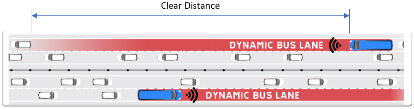
Illustration of the dynamic bus lane (DBL) concept.
Wu et al. ( 3 ) studied the efficiency of DBLs under different clear distances ahead of the bus. They showed that the optimum clear distance that improves traffic and transit performance is 150 m and that increasing the clear distance can significantly deteriorate traffic performance (speed) with minor improvement in transit speed. Thus, a length of 150 m is a balanced solution that achieves improved traffic and transit performance. Additionally, the results showed that DBLs under the optimum clear distance can reduce the average person delay by 55% to 72% when compared with EBLs, allowing for better utilization of the available lane capacity ( 3 ). Zhao and Zhou ( 22 ) studied the impact of DBLs on traffic and transit performance for a corridor in Shanghai, China. This study compared the average person delay for traffic and transit users for three cases: the case of no control, EBLs, and DBLs. The results showed that DBLs can reduce the average person delay by 5% and 10% when compared with no prioritization and EBL strategies, respectively ( 22 ). A recent study by Szarata et al. ( 23 ) evaluated the impact of DBLs on traffic and transit performance for four different corridors in Rzeszów, Poland, using using a microsimulation model. The study found that EBLs increased the average travel time for the general traffic by 25%, while the average travel time increased by 1% in the case of DBLs. Additionally, EBLs could increase the overall person delay by more than 10%, while DBLs have the potential to reduce the overall person delay by 8% to 10% ( 23 ).
Although the impact of DBLs is investigated in the above recent studies, some important gaps can be identified and warrant further investigation. For example, drastically different results are reported across the previous studies. While some studies report that DBLs can improve the corridor performance by 5% ( 22 ), other studies show that DBLs can improve the corridor performance by more than 20% ( 3 ). The main factor causing this discrepancy is that all previous studies focus on testing the impact of DBLs under different conditions of traffic demand and transit frequency, which poses the need for a comprehensive analysis of the impact of DBLs on the corridor performance. For example, it is not clear under what conditions DBLs can be considered the most effective solution for improving the overall corridor performance. In other words, it is unknown how DBLs perform under different traffic demand and different transit frequency levels in comparison with EBLs and the case of no prioritization. In this study, a comprehensive analysis is conducted to investigate the effectiveness of DBLs under a wide range of possibilities (different demand and different frequencies). Additionally, it is not clear what is the best criterion to judge the impacts; that is, the impact on transit delays, traffic delays, or combined person delays. Lastly, the negative impact of transit lanes on traffic can be justified only if the resulting enhanced transit service induces sufficient mode shift to transit. Therefore, assessment of the full impact of DBLs and EBLs must consider the potential for mode shift from driving to transit, even with simple but reasonable assumptions based on knowledge of mode shifts from field observations of EBLs. Altogether, such comprehensive sensitivity analysis is important for evidence-based decision making as neither DBL nor EBL is a clear winner under all conditions, as is quantitatively demonstrated later in the paper. DBL is clearly a promising technology-enabled strategy, and therefore comprehensive guidelines for its implementation in the connected environment and an approach to quantify the corresponding impact on traffic flow and road capacity are needed. Thus, this paper investigates the impact of DBLs and EBLs versus no transit lane on: (i) transit speed performance, (ii) traffic speed performance, and (iii) total person travel time performance, under different traffic demand and transit frequency levels and mode shift assumptions. This study shows which strategy is the most efficient and applicable under what conditions. The results of this study complement prior efforts and offer a basis for researchers, traffic and transit practitioners, and authorities to assess the potential of DBLs and avoid the potential pitfalls of EBL implementation.
Methodology
Case Study and Characteristics of the Selected Corridor
The City of Toronto recognizes the necessity of improving transit services to achieve the city’s vision for a sustainable future. Thus, the city authorities recognize that surface transit priority plays a key role in these improvements. In 2019, the Toronto Transit Commission (TTC) approved a five-year service plan, which identified five corridors for the implementation of EBLs: Eglinton East, Jane Street, Dufferin Street, Finch Avenue West, and Steeles Avenue West, as shown in Figure 2a. These are among the most heavily-used transit corridors serving about one quarter of a million riders every weekday (pre-COVID conditions). Additionally, these corridors provide service all day, seven days a week, and they accommodate heavy vehicle traffic (especially during the peak hours) ( 24 ). The first implementation of EBL, along the Eglinton East corridor, commenced in 2020. Thus, Eglinton East corridor was selected as the case study in this research for investigating the relative impacts of DBLs, EBLs, and no bus priority. The Eglinton East corridor is 11 km in length and runs from Kennedy Subway Station to the University of Toronto Scarborough Campus (UTSC). Multiple TTC bus routes operate on the corridor, and the average bus speed in the peak periods is 18.5 km/h, which is a relatively low speed when compared with the average traffic speed of about 34 km/h. The pavement width of the corridor varies from 15 m (two lanes per direction) to 27 m (three lanes per direction) as shown in Figure 2b. The available right of way does not allow for the implementation of a new lane to be dedicated to transit. Additionally, reducing the lane width to the minimum guidelines and removing median two-way left-turn lanes does not offer the required space for the implementation of the bus lanes in the two directions. Thus, it is not feasible to implement the bus lane and maintain the same number of lanes for the general traffic. Therefore, one of the existing traffic lanes per direction was converted into an EBL, reducing the number of lanes available for the general traffic and introducing some bottlenecks where only one traffic lane is left.
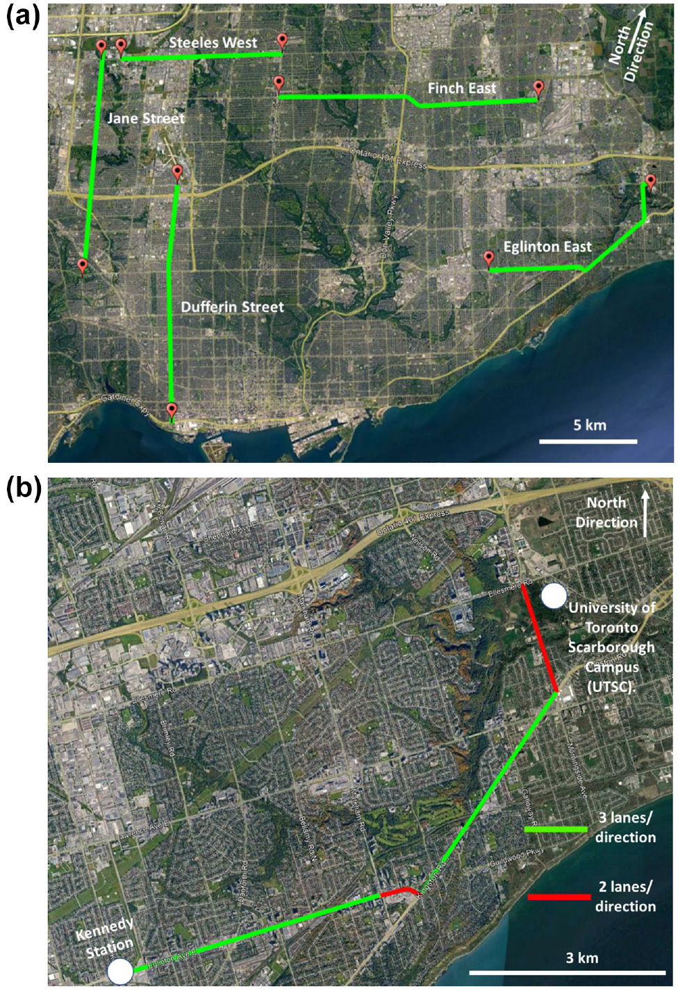
RapidTO exclusive bus lane (EBL) plan identified by the (TTC) five-year service plan: (a) RapidTO corridors for implementation of EBL and (b) Eglinton East corridor with the number of lanes available before the implementation of the EBLs.
Microsimulation Traffic Model and the Calibration Process
Three microsimulation traffic models were developed using Aimsun Next for the three strategies tested (DBL, EBL, and no priority) for the morning peak period (6:00 to 9:00 a.m.) in Eglinton East corridor. The traffic demand in the models was defined as origin–destination (OD) matrices which were developed using data from the 2016 Transportation Tomorrow Survey ( 25 ). However, the 2019 turning movement counts are available online on the open data portal provided by the City of Toronto ( 26 ). Thus, the Webster method was used for optimizing the signal phasing timings based on the 2019 turning movement counts. Additionally, the OD matrices in the subnetwork were calibrated based on the morning peak (6:00 to 9:00 a.m.) turning movement counts in 2019 (pre-COVID conditions) using the OD adjustment tool available in Aimsun. For the intersections, Google Maps was used to provide detailed information on the number of lanes of each approach, the existence of turning lanes (right-turn lanes and left-turn lanes), the length of the turning lanes (if any), the locations of the stop lines, the lengths of the solid lines used for preventing lane changing, and the direction of travel for each lane. Furthermore, bus lines and their routes were defined, including their schedules, headway, and dwell time based on the TTC published report ( 24 ). The average traffic speed of the final calibrated model (for the case of no priority) is 32.71 km/h, while the average traffic speed reported by TTC ( 24 ) is 34 km/h (3.8% error). Additionally, the average transit speed of the calibrated model is 18.87 km/h, while the average transit speed reported by TTC is 18.5 km/h (2% error).
For DBLs, the traffic management tool in Aimsun was used for modeling this strategy. The tool allows for modifying the traffic network conditions, influencing the driving behavior, or simulating events on the traffic network. Thus, this tool was used to enforce a lane closure for a specific length ahead of the bus in a dynamic fashion. In other words, at every simulation step (1 s), the simulation model uses the real-time information for the locations of the buses and enforces a lane closure for a specific distance (clear distance) ahead of every bus in the model, and lane changing is necessary for any vehicle in the clear distance to exit. In some cases, the lane-changing might not be possible because of the unavailability of a sufficient gap in the adjacent lane. Thus, it is expected that the performance of the DBL will be similar to the no control scenario for congested networks. In this case, the vehicle will continue to travel in the bus lane until a sufficient gap is found in the adjacent lane. To select an appropriate clear distance that achieves the best corridor performance for both transit and traffic, a sensitivity analysis was conducted to estimate the total person travel time in the corridor at different values of the clear distance in the calibrated model. The clear distance values tested start from a distance of zero, which represents the case of no priority, to a distance of 500 m with an increment of 50 m. Additionally, the case of EBLs was tested and the total person travel time for this case was estimated. Figure 3 shows the relationship between the clear distance and the total person travel time. The figure shows that the total person travel time decreases with the increase in the clear distance until the minimum total person travel time is reached at a clear distance of 150 m. The total person travel time then slightly increases at a clear distance of 200 m and at a faster rate thereafter. A detailed discussion and explanation of the impact of DBLs and EBLs on the total person travel time will be provided in the analysis section. These results are compatible with the results of the study by Wu et al. ( 3 ) which showed that 150 m is the clear distance that optimizes both transit and traffic speeds. As a result, a clear distance of 150 m is used for the case of DBLs in the remainder of this paper. However, it must be mentioned that the clear distance is potentially a function of both traffic demand and transit frequency. Thus, further research is needed to advance the concept of DBLs by developing intelligent algorithms for adaptively determining the settings of such a strategy in real time.
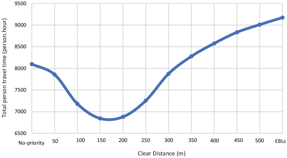
Total person travel time for the calibrated model under different clear distances.
Additionally, to analyze and compare the three scenarios, the following assumptions were made:
No changes in the route choice (no vehicles will be attracted or changing their route preference). This assumption was made to test and compare the effectiveness of the three strategies under the same conditions.
The network topology was not examined.
The rate of connected vehicles (CVs) is 100%.
The rate of compliance is 100%.
Bus occupancy = 50 passenger/bus (as this is one of the most heavily-used transit corridors in the City of Toronto as stated by the TTC [24]).
Car occupancy = 1.25 person/vehicle (which is the average occupancy in the morning peak period in Toronto as reported by the Transportation Tomorrow Survey [25].)
Since the main objective of this study is to analyze comprehensively the impact of DBLs and EBLs on traffic and transit under different demand and frequency levels, 10 different traffic demand levels were introduced to the network as multiples of the calibrated OD matrix starting with a demand of 0.2 of the original demand (0.2D) and increasing to twice the original demand (2D) with increments of 0.2 D. Additionally, 21 different transit frequency levels were tested under every demand level. The frequencies tested start from high frequency service of 30 buses per hour (buses/h) or 2 min headway to six buses per hour or 10 min headway with an increment of 0.5 min headway. Low frequencies were then tested using the clock headways of 12, 15, 20, and 30 min, which are equivalent to frequencies of two, three, four, and five buses/h. Thus, a total of (21 × 10 =) 210 cases of different traffic demand and frequency levels are tested. For each case, 10 simulation replications were employed to reflect the stochastic nature of simulation, and the outputs reported in the next section are the average values of these 10 runs. Thus, a total of 2,100 simulation runs were employed for evaluating the impact of DBLs. Additionally, the same simulation runs were repeated for the case of EBLs and no bus priority to compare their performance with the performance of DBLs. Thus, a total of 2,100 × 3 = 6,300 simulation runs were completed to comprehensively analyze the impacts of DBLs and compare the effectiveness of this strategy with EBLs and no bus priority conditions. The analyses were conducted under multiple different mode shift assumptions (or percentages). At one extreme, it is assumed that no mode shift occurs when the transit lanes (DBL or EBL) are introduced. At the other extreme, it is assumed that travelers will shift from driving to transit to consume all the extra transit capacity gained from the higher frequency because of the reduced cycle time.
Analysis and Discussion
Analysis of the Average Transit Speed
The average bus speeds for the three tested scenarios (no priority, EBL, DBL) are shown in Figure 4 and a comparison of the average bus speeds across the three scenarios is shown in Figure 5. In the case of no priority, the results show that the average bus speed decreases with the increase in the traffic demand in the network. For the case of EBLs, the average bus speed remains consistent (around 20 km/h) across all cases as buses are not affected by the surrounding traffic. For the case of DBLs, the average bus speed decreases with the increase in the traffic demand in the network, which is similar to the pattern of the case of no priority but milder. Under low traffic demand, the average bus speeds for the cases of DBLs and no priority are very close to each other and to the case of EBLs. However, the average bus speed in the DBL scenario is higher than the average bus speed in the no priority scenario under intermediate and heavy traffic volumes and this difference can reach up to 35% and 15% under intermediate and heavy traffic demand, respectively. Additionally, under intermediate traffic demand, the average bus speeds in the DBLs and no priority scenarios are respectively 4% and 15% lower than the average bus speed in the EBL scenario, and these percentages reach up to 35% and 55% under heavy traffic demand.
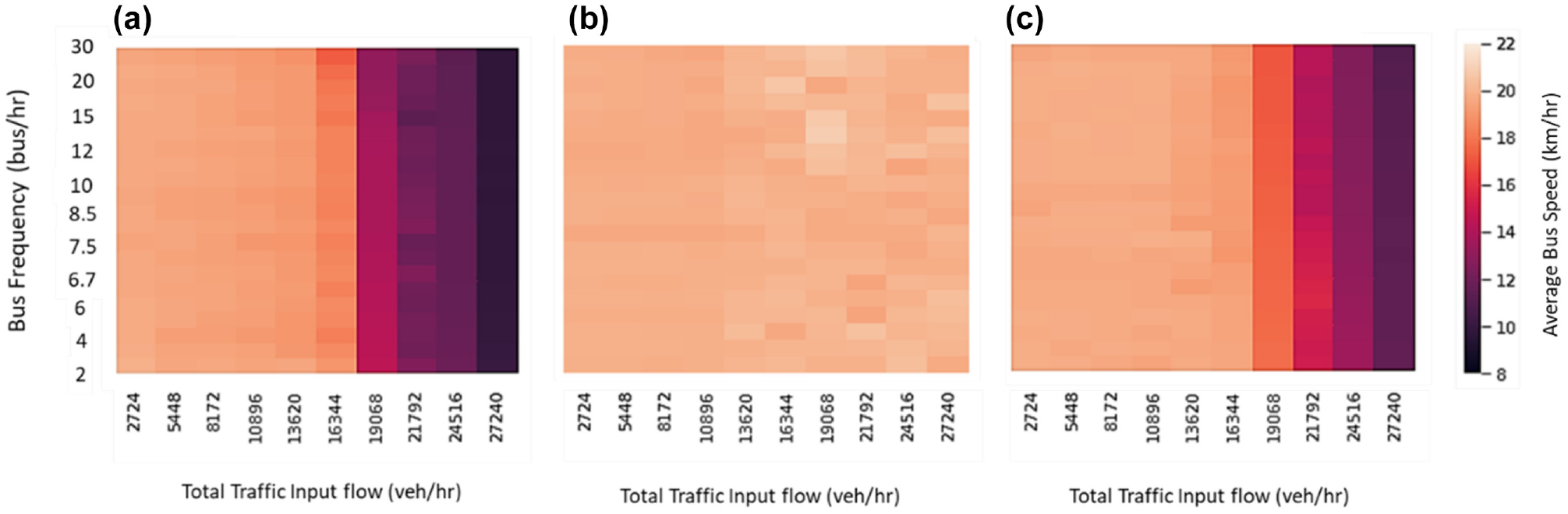
Average bus speed (km/h) for the three tested scenarios: (a) no priority, (b) exclusive bus lanes (EBLs), and (c) dynamic bus lanes (DBLs).
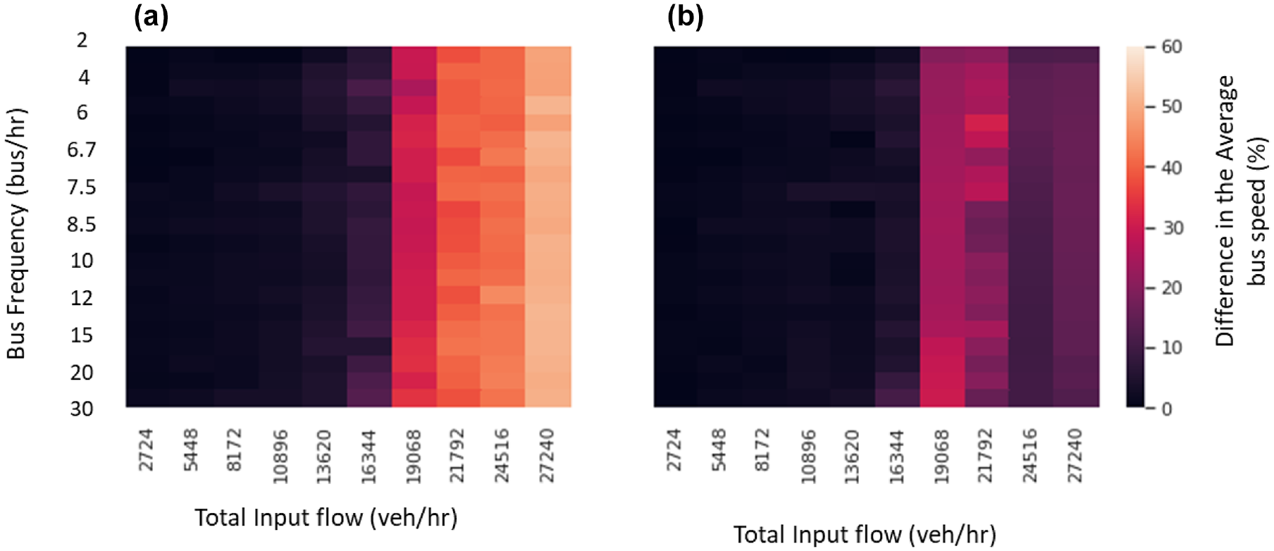
Percent difference in the average bus speed between the three strategies: (a) exclusive bus lanes (EBLs) versus no priority and (b) dynamic bus lanes (DBLs) versus no priority.
Analysis of the Average Traffic Speed
The average traffic speeds for the three tested scenarios (no priority, EBL, DBL) are shown in Figure 6, and a comparison of the average bus speeds across the three scenarios is shown in Figure 7. The three scenarios have the same pattern as the average traffic speed, which decreases with increase in the traffic demand, while the EBL case is the worst, followed by the DBL case then the mixed traffic case, which is intuitive. Under low traffic demand, the average traffic speed remains almost the same in all scenarios. However, under intermediate traffic demand, the average traffic speed for DBLs depends on the transit service frequency because higher frequencies mean higher number of running buses with associated priority length that cannot be used by cars, thus affecting the average traffic speed. In the cases of low transit frequencies, the average traffic speed in the DBL scenario is very close to the average traffic speed in the case of no priority, with the difference ranging between 1% and 4%. In the cases of high transit frequencies, the average traffic speed in the DBL scenario is 7% to 15% lower than the average traffic speed in the no priority scenario. Under heavy traffic demand, the difference in the average traffic speeds between the no priority and DBL scenarios decreases, reaching from 2% (under low frequencies) to 9% (under high frequencies). Thus, for the cases of low frequencies, the average traffic speeds in the DBL scenarios, under all demand levels, are similar to the average traffic speed for the no control scenario. However, for the cases of high frequencies, the difference in the traffic speed between the DBL and no priority scenarios increases because of the increase in the number of buses with their clear length that the general traffic cannot use. Additionally, in the cases of high frequency, the difference in the average traffic speed between the case of DBL and no priority increases moving from low to intermediate traffic volumes. However, this difference decreases again moving from intermediate to heavy traffic volumes. This reduction happens because, under heavy traffic volumes, the network becomes more congested and in these cases the probability that a bus arrives at a congested section increases and the vehicles ahead of the bus cannot clear the bus lane and switch to the adjacent lane as there is not enough space or gap for the maneuver. Thus, the bus has to wait in the queue and will not receive the desired priority. The previous phenomenon can also be noticed in the previous subsection (“Analysis of the Average Transit Speed”) when the average bus speeds for the cases of DBL and no priority were compared. The results show that the difference in the average bus speeds in the two cases increases, reaching up to 35% in intermediate traffic conditions but under heavy traffic this difference decreases to 15%. Additionally, when the average bus speeds in the DBL and EBL were compared (in the previous subsection), the results show that this difference increased from 4% under intermediate traffic volume to 40% under heavy traffic volumes, which means that the DBL allows the buses to travel near the free-flow speed similar to the case of EBL under intermediate traffic. However, under heavy traffic volumes the ability of the DBL to give the desired priority to the buses declines.
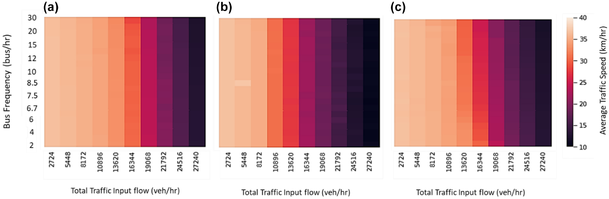
Average traffic speed (km/h) for three scenarios tested: (a) no priority, (b) exclusive bus lanes (EBLs), and (c) dynamic bus lanes (DBLs).
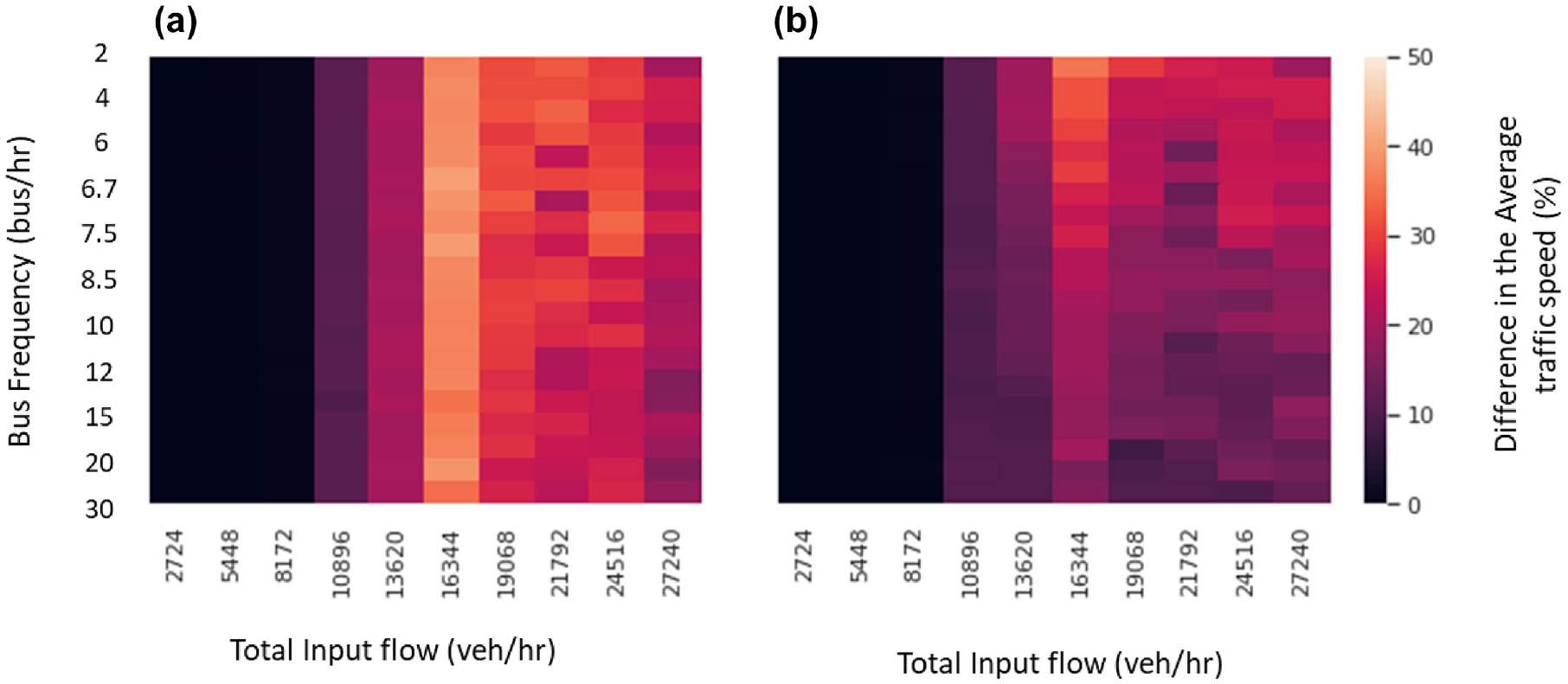
Percent difference in the average traffic speed between the three strategies: (a) no priority versus exclusive bus lanes (EBLs) and (b) dynamic bus lanes (DBLs) versus EBLs.
Finally, under intermediate traffic demand, the average traffic speeds in the DBL and no priority scenarios are respectively 35% and 42% higher than the average traffic speed in the EBL scenario and, these percentages remain high at 25% and 35% under heavy traffic demand. This significant difference in the speeds occurs because of the reduction in the available capacity for the general traffic. Thus, although EBL and DBL prioritize transit service and improve the average bus speed when compared with the case of no control, the impact of the DBL strategy on the general traffic, under intermediate and heavy traffic conditions, is minor when compared with the impact of the EBL on the surrounding traffic.
Comparative Analysis of the Overall User Impacts of the Three Strategies
The comparison is divided into two stages as follows:
Stage 1: does not take into account the changes in the mode choice and compares the three strategies under the same conditions (the same traffic demand and the same transit frequency) assuming that travelers will not switch from one mode to another (without any changes in the original OD matrices).
Stage 2: this stage takes into consideration the impact of improving the transit service on mode choice. In other words, providing a transit improvement strategy causes improvement in the bus speed and in turn reduces the cycle time, which increases the service frequency for the same fleet size, reducing the waiting time and increasing the route capacity. In this stage, it is assumed that the additional capacity resulting from any transit improvement strategy will be totally utilized by new riders switching from passenger vehicles. As a result, vehicular traffic volumes would be reduced accordingly with the assumption that there are no changes in the original OD matrices.
Thus, stage 1 represents one extreme in which no change in mode choice behavior would occur, while stage 2 represents the other extreme as the entire additional transit capacity (resulting from any transit improvement strategy) would be fully utilized by travelers switching from using passenger vehicles. The real-life scenario is expected to be somewhere between these two extremes.
Stage 1: No Changes in the Mode Choice
In this section, the performance of each strategy is compared with the other strategies using the total person delay under the same traffic demand and transit frequency conditions assuming no changes in the mode choice between the three scenarios (no change in the mode choice or route choice). The total person delay is calculated as the delay of all travelers in the corridor (transit and traffic) using Equation 1. Additionally, it must be mentioned that at this stage (stage 1) the delay-based analysis would yield the same results as person travel time-based analysis, since it is assumed that EBLs and DBLs would not cause any benefits to the waiting time as the frequencies are kept the same across the three scenarios (EBL, DBL, and no priority).
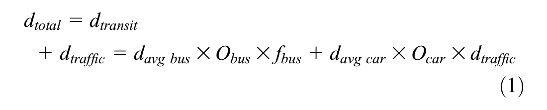
where
The total person delay for every condition tested for the three tested scenarios (no priority, EBL, DBL) is shown in Figure 8. The three scenarios have the same pattern as the total delay increases with the increase in the traffic demand. However, EBL is the strategy that achieves the highest total person delay across all scenarios. That is, under no condition is EBL justifiable based on total person delays. To visualize the results, Figure 9 shows the percent difference in the total person delay between the EBL and DBL scenarios and the no priority scenario. Figure 9a shows that the difference in the total person delay between the EBL and no priority scenarios increases with the increase in the traffic demand, and EBL can deteriorate the overall person delay by up to 60% and 70% under intermediate traffic demand and 30% to 40% under heavy traffic demand. On the other hand, DBL can reduce the overall person delay by 25% and 5% under intermediate and heavy traffic demand, as shown in Figure 9b. Under intermediate traffic demand, the difference in the total person delay between the DBL and no priority scenarios depends on the transit frequency. Under intermediate traffic demand and low frequencies, the improvement in the total person delay is minor (less than 5%). On the other hand, under high transit frequency, DBL can improve the overall person delay by 20% to 25% as DBLs allow the buses to travel at the free-flow speed and at the same time let the general traffic travel at high speed similar to the case of no bus priority. Under heavy traffic demand, the impact of DBL on the total person delay decreases and reaches 2% under low transit frequencies, while this percentage reaches 5% to 8% under high frequency services. Thus, based on the total person delay, the optimum strategy, that minimizes the overall person delay on the corridor, under every traffic and demand level can be identified. It is assumed that any transit prioritization strategy (EBL or DBL) will be considered the optimum strategy if it can improve the overall person delay by more than 5% to justify the implementation cost of the strategy. Figure 10 shows the optimum strategy under various conditions. Under low traffic demand, the implementation of any transit improvement strategies is not justified as they do not result in improvements in the overall person delay. Under intermediate and heavy traffic demand, the optimum strategy depends on the transit frequency as the optimum strategy under low frequency is no priority, while the optimum strategy under high frequency is DBL. On the other hand, EBL does not appear in the figure as EBLs improve the corridor performance for transit users, while they substantially deteriorate the performance for the general traffic because of the reduction in road capacity. Thus, EBLs result in a major increase in the overall person delay under intermediate and heavy traffic demand. On the other hand, DBL is the most favorable strategy in most cases under the intermediate and heavy traffic conditions as this strategy gives priority to transit vehicles while allowing traffic to use the lane when there is no bus in the lane.
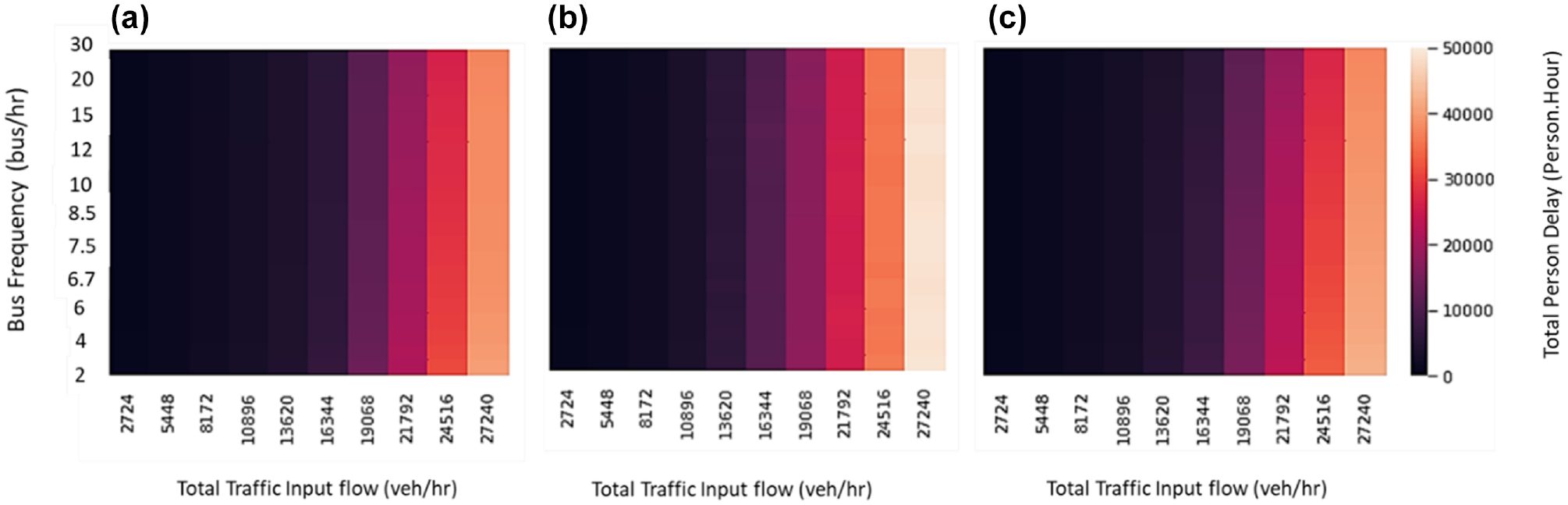
Total person delay over the three simulation hours (hr) for three different scenarios tested: (a) no priority, (b) exclusive bus lanes (EBLs), and (c) dynamic bus lanes (DBLs).
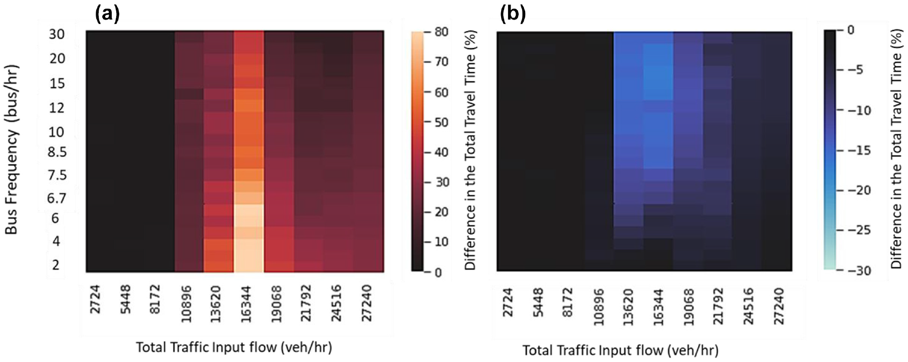
Percent difference in total person delay between the three strategies: (a) exclusive bus lanes (EBLs) versus no priority and (b) dynamic bus lanes (DBLs) versus no priority.
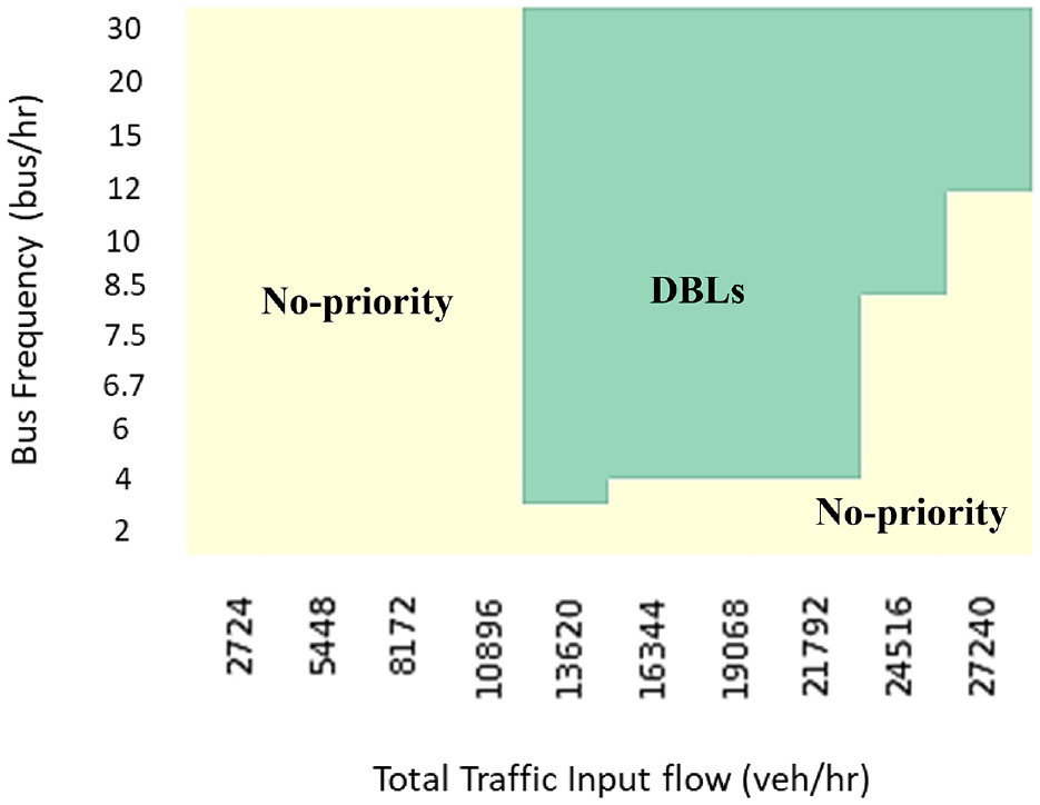
The optimum strategy under various demand and frequency levels assuming no mode shift.
Stage 2: Considering Changes in the Mode Choice
The previous analysis compared the three strategies under the same traffic demand and frequency levels assuming no change in the mode choice, which is one extreme case. Under this assumption, it is clear that EBLs lead to a significant reduction in road capacity for the other road users and consequently have a non-trivial negative impact on traffic. Such negative impact on traffic is often tolerated/justified by system operators in the hope that it will induce mode shift to transit. If the enhanced transit performance does not induce mode shift from driving to transit, the net effect of EBL on all users in total person delay is consistently negative. However, it is reasonable to expect that any improvement in the transit service will result in an improvement in the transit service performance and induce behavioral changes. In this analysis, first, the required fleet size is calculated under each combination of traffic demand and frequency levels for the no priority scenario (considered as the base case scenario) using the average bus speed. Any improvement strategy (EBL or DBL) would then increase the average bus speed and in turn reduce the cycle time, thus increasing the service frequency using the same fleet size. Increase in bus frequency increases the transit route capacity and thus attracts more riders in a virtuous cycle. In this section, it is assumed that the additional transit capacity achieved will be utilized fully by new riders switching from using passenger vehicles to transit, and this applies to all combinations of baseline traffic demand and frequency levels. Accordingly, the reduction in traffic demand would be equivalent to the increase in route capacity. Additionally, increasing the bus frequency (given the reduced cycle time) would reduce the waiting time for transit users. To take into account the impact of the waiting time, the comparison in this section focuses on the total travel time instead of the overall person delay (as in the previous subsection) as the overall person delay only considers the in-vehicle travel time. Generally, people perceive their waiting time to be considerably much longer than the actual waiting time. Different surveys provided different ratios of waiting time to in-vehicle time ( 27 ). For example, Wardman ( 28 ) found that waiting for transit for 1 min is equivalent to 2.5 min of in-vehicle time. Horowitz ( 29 ) found that the ratio is 1.9. Abrantes and Wardman ( 30 ) found that waiting for transit for 1 min is equivalent to 1.4 min in-vehicle. Consequently, in the present analysis, the ratio of waiting time to in-vehicle travel time is assumed to be 2. Moreover, the waiting time for high frequency services (with a headway of 10 min or less) is calculated using Equation 2 and the waiting time for low frequency services (with headway more than 10 min) is calculated using the model by Fan and Machemehl ( 31 ) shown in Equation 3.


Finally, the total travel times for all travelers in the corridor are calculated and compared to find the optimum strategy that minimizes the overall travel time in the network for all transit and traffic users under different conditions. To visualize the results, Figure 11 shows the percent difference in the total person travel time of the EBL and DBL scenarios to the no priority scenario. Figure 11a shows that EBLs do not improve the total travel time in low traffic demand conditions. Under intermediate traffic demand, the average bus speed in the case of no priority is similar to the average bus speed for the case of EBLs (the first few columns in the intermediate traffic demands), and therefore EBLs offer almost no additional transit capacity. Accordingly, introducing an EBL under such conditions would increase the overall person travel time in the corridor by up to 20%. On the other hand, when there is a difference in the average bus speeds between the two scenarios (the last few columns in the intermediate traffic demand), EBLs would improve the average bus speed, and subsequently improve the service frequency/capacity, reduce the average waiting time, and attract the general auto users, thus reducing the overall person travel time in the corridor. The magnitude of reduction in the total travel time increases as we move from low frequency service to high frequency service. The results show that EBLs, under intermediate traffic level, increase the total person travel time by 5% under low frequencies and reduce the total person travel time by 5% under high frequencies. In heavy traffic demand, the same pattern can be noticed as EBLs increase the total travel time by 5% to 10% under low frequency services and reduce the total travel time by 15% to 20% under high frequency services.
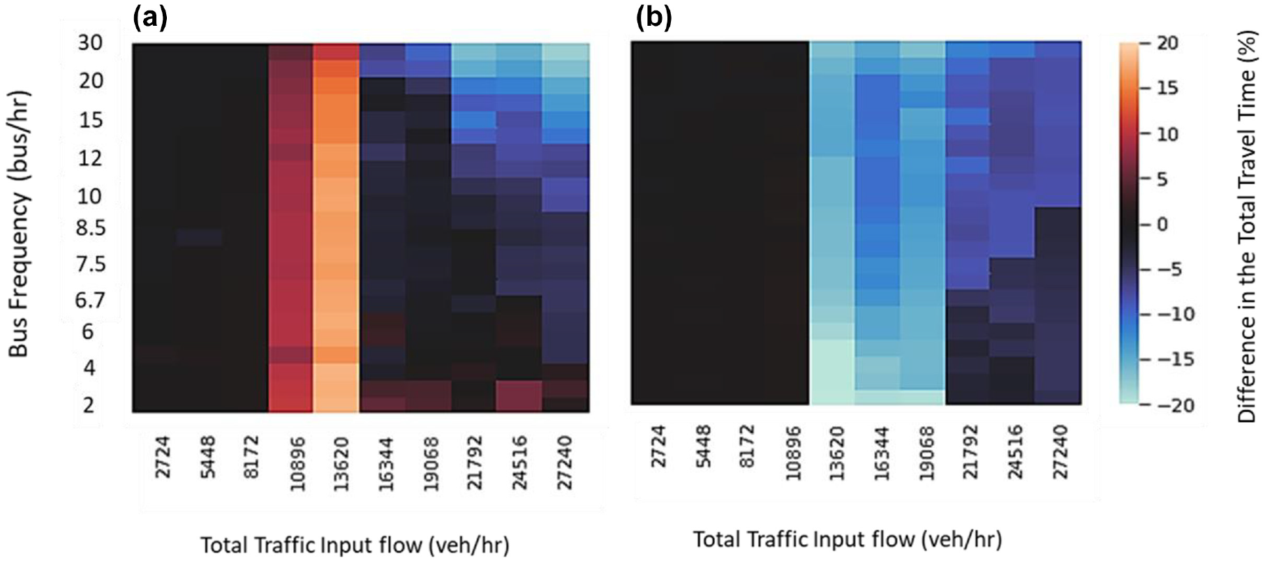
Percent difference in total person travel time between the two strategies: (a) exclusive bus lanes (EBLs) versus no priority and (b) dynamic bus lanes (DBLs) versus no priority.
On the other hand, DBLs show a large reduction in the total person travel time under intermediate traffic levels by up to 20%. For heavy traffic demand, DBLs can achieve minor improvement in the total person travel time of less than 5% under low frequencies. However, the magnitude of this improvement increases with the increase in the transit service frequency and can reach up to 10% to 15%. Thus, based on the total person travel time in the entire corridor, the optimum strategy that minimizes the overall person delay on the corridor under every traffic and demand level can be identified. It is assumed that any transit prioritization strategy (EBL or DBL) will be the optimum strategy if the strategy can improve the overall person travel time by more than 5% to justify the implementation cost of the strategy. Figure 12, the most important figure in this analysis, shows the optimum strategies under the different conditions. Under low traffic demand, the implementation of any transit improvement strategy is not justified as it would not result in improvements in the overall person delay. Under intermediate traffic demand, DBL is the optimum strategy as it minimizes the overall travel time in the corridor. Under heavy traffic demand, the optimum strategy depends on the transit frequency: under low, intermediate, and high frequency, the optimum strategies are no priority, DBL, and EBL, respectively. Unlike the analysis of stage 1, EBL with optimistic mode shift is the optimum strategy in the extreme cases of highest demand and highest transit frequencies, as it is assumed that some of the general traffic will switch from driving to using buses and thus the traffic demand will be reduced as a result of this mode shift, and the impact of the EBLs on the general traffic will not be as aggressive as it was in the previous analysis.
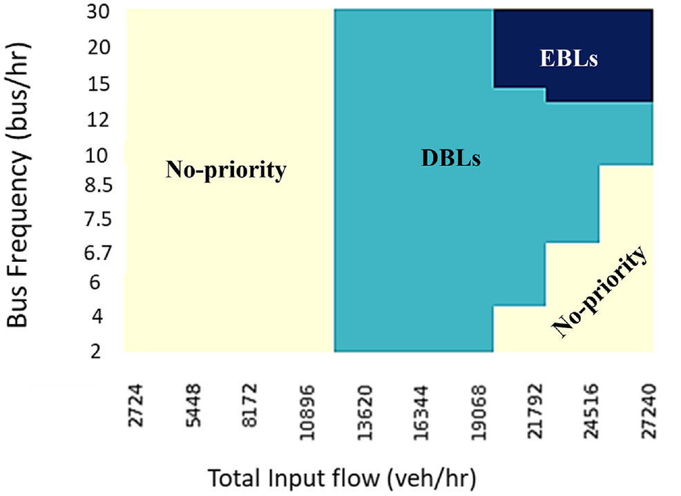
The optimum strategy under various demand and frequency levels assuming mode shift.
Finally, it was mentioned in the introduction that drastically different results are reported across the previous studies that analyzed the impacts of DBLs. While some studies report that DBLs can improve the corridor performance by 5%, others show improvements of more than 20%. The main factor that causes this discrepancy is that all the previous studies focus on testing the impact of DBLs under certain conditions (certain traffic demand and certain transit frequency), which is a single condition out of the 210 conditions (demands and frequencies) tested in this paper. Additionally, the present analysis shows that DBLs can improve the corridor performance by different percentages under every traffic demand and transit frequency levels, as shown in Figure 11b.
Mode Shift Sensitivity Analysis
Although a mode shift model is desired to capture the impact of the implementation of DBLs on the mode choice and in turn on the corridor performance, DBL is an emerging strategy with very few implementations around the world, and as such no revealed data is available to support a mode choice model. One alternative is to build a model based on stated preference experiments, which lies beyond the scope of this study. The previous section investigated the impact of DBLs and EBLs on the corridor performance under two mode choice assumptions (no change in the mode shift or full utilization of the additional bus capacity). On the other hand, this section focuses on analyzing the impact of DBLs and EBLs on the corridor performance under different mode shift percentages starting from the assumption of no mode shift (0%) to full utilization of the additional bus capacity (100%) with increments of 25%. In other words, the impact of DBLs and EBLs on the corridor performance will be investigated with 0%, 25%, 50%, 75%, and 100% utilization of the additional bus capacity resulting from the improvement in the bus speed. The total person travel time for every mode shift tested is then calculated, for all the demands and frequencies assumed, the same way the analysis in stage 2 was conducted. Figure 13 shows the optimum strategy under the different conditions for every mode shift percentage. The figure shows that the areas of efficiency of DBLs and EBLs increase, moving from 0% mode shift to 100% mode shift because the increase in the mode shift percentages can be translated into a lower number of vehicles on the corridor and in turn better conditions. Thus, there is a gradual increase in the areas where DBLs and EBLs are the efficient strategies, that minimizes the total person travel time in the corridor, from the no mode shift to the 100% mode shift.
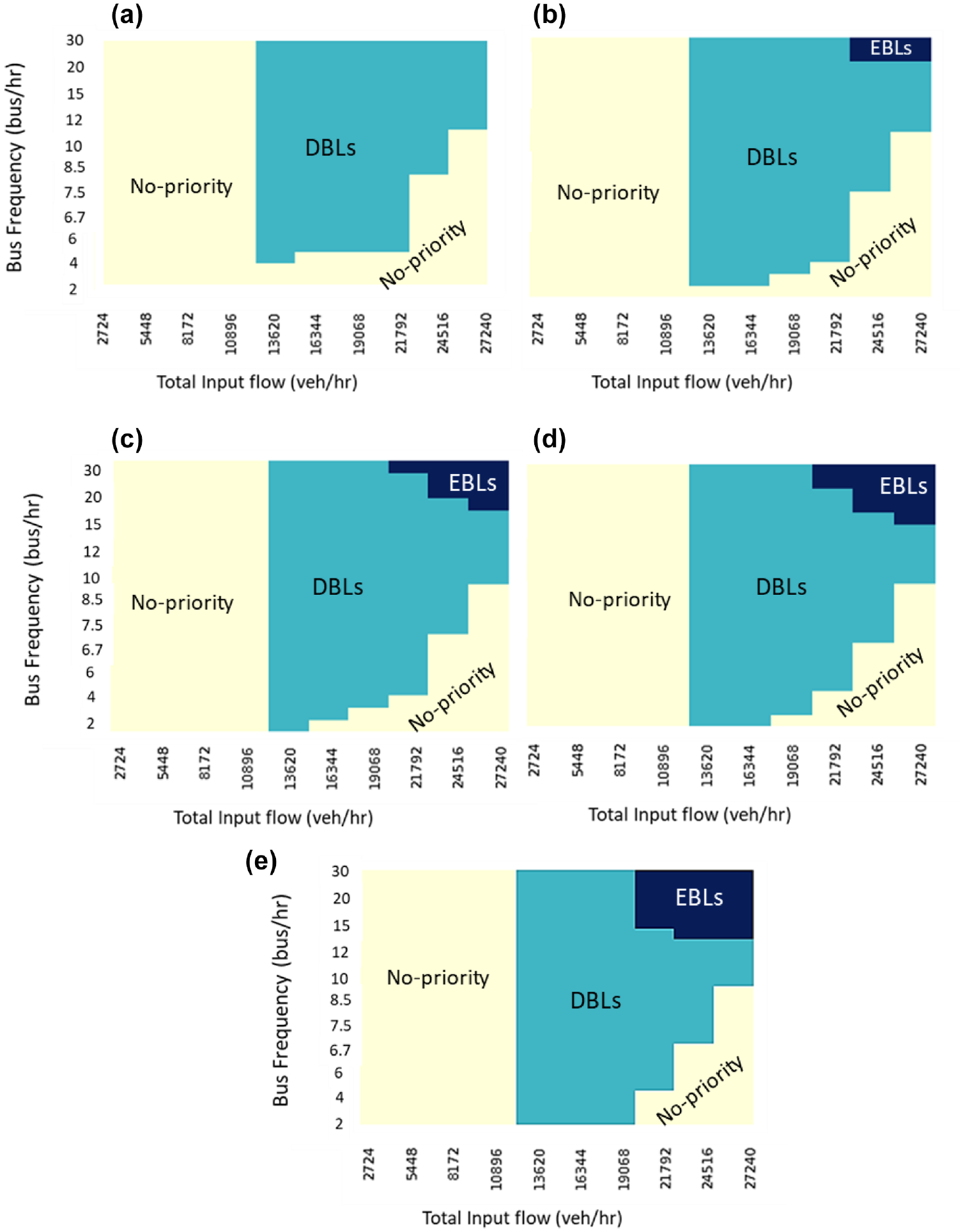
The optimum strategy under various demand and frequency levels assuming different mode shift percentages: (a) 0%, (b) 25%, (c) 50%, (d) 75%, and (e) 100%.
Conclusion
Dynamic transit lanes are priority lanes that are accessible to the general traffic when transit is not present. A simulation model of the Eglinton East corridor in Toronto was built to investigate the impact of DBL, EBL, and no priority strategies on the performance of public transit and the general traffic under different traffic demand and transit frequency levels. The following conclusions can be drawn from the conducted analysis:
When traffic demand is high, the introduction of EBLs can improve the average bus speed but deteriorate the average traffic speed, causing substantial increase in the total person delay if no mode shift to transit occurs. On the other hand, DBLs can improve the average bus speed, similar to EBLs, with less impact on the general traffic because this strategy provides priority to buses only at locations where buses are present, thus minimizing the impact on adjacent traffic. The analysis shows that DBLs can be more effective than the traditional strategies (no priority or EBL) over a wide range of traffic and transit service conditions, as shown in Figures 9 and 11.
Under low traffic demand conditions, DBL, EBL, and no priority strategies offer the same corridor performance. Thus, no transit prioritization strategy is needed.
Assuming no behavioral change (no change in the mode choice), EBLs will always deteriorate the overall performance of the corridor when compared with the case of no priority. On the other hand, DBL is the optimum strategy that improves the corridor performance under intermediate traffic demand and heavy traffic demand with high frequency services.
Taking into account optimism about changes in the mode choice, EBL is the optimum strategy that minimizes the total person travel time in the corridor only under heavy traffic demand and high transit frequency services. On the other hand, DBL is the optimum strategy under intermediate traffic demand and heavy traffic demands with intermediate transit frequency.
While this study offers useful insights for researchers, traffic and transit practitioners, and authorities on the relative performance of DBLs and EBLs, more research is needed to confirm the findings of the study by replicating it in other case studies. Additionally, further research is needed to advance the concept of DBL by developing intelligent algorithms for adaptively determining the settings of such a strategy in real time. In other words, an algorithm is needed that determines the optimum clear distance ahead of the bus taking into consideration the current bus and traffic status. These algorithms can be thought of as “adaptive transit lanes” where the clear length ahead of the bus is not fixed but rather changes from section to section according to the bus status and traffic conditions. Furthermore, the impact of DBLs on route performance depends largely on the compliance rate, which is influenced by several factors including the level of connectivity between buses and downstream vehicular traffic, the behavior of general traffic drivers, and enforcement protocols. Thus, further research is needed to understand the impact of compliance and associated factors on the efficiency of DBLs.
Footnotes
Author Contributions
The authors confirm contribution to the paper as follows: study conception and design: K. Othman, A. Shalaby, B. Abdulahi; data collection: K. Othman, A. Shalaby; analysis and interpretation of results: K. Othman, A. Shalaby, B. Abdulahi; draft manuscript preparation: K. Othman, A. Shalaby, B. Abbdulahi. All authors reviewed the results and approved the final version of the manuscript.
Declaration of Conflicting Interests
The author(s) declared no potential conflicts of interest with respect to the research, authorship, and/or publication of this article.
Funding
The author(s) disclosed receipt of the following financial support for the research, authorship, and/or publication of this article: This research is funded by Huawei Canada Research Centre.