Advisory-Based Time Slot Management System to Mitigate Waiting Time at Container Terminal Gates

Abstract

This paper introduces an advisory-based time slot management system (TSMS) to control truck arrivals at seaport terminals with the aim to reduce congestion at terminal gates. A modeling framework is proposed, developed, and applied to assess the impact of a truck arrival shift for a case study in the Port of Rotterdam. This system is designed to apply control policies on truck inflow while taking the behavioral aspect of truck operating companies (TOCs) into account. Discrete choice modeling is used to infer the time-of-day preferences of TOCs for container pick-ups from the exchange of information between port and hinterland stakeholders. These preferences are used to shift truck arrivals to the off-peak period which consequently reduces the high waiting time of trucks at terminals gates. To evaluate the effectiveness of the designed TSMS, a simulation platform that resembles terminal operations has been developed using discrete-event simulation. For the allocation of trucks to a certain time of day, a choice-based stochastic assignment heuristic is designed to approximate the optimum configuration of the truck arrival shift policy experiment. The optimum truck arrival shift design shows that significant gain can be obtained even at a low shift rate.

High waiting time for trucks at the terminal gates of seaports is an issue that is increasingly receiving more attention. Long queues of idling trucks at terminal gates waiting to pick up or deliver a container lead to congestion further upstream, and induce emissions, costs, and delays ( 1 – 4 ). Container terminals in the Port of Rotterdam area—the largest European port—are no exception to these issues, as the waiting time for trucks at the terminal gates has been rapidly increasing over the past 6 years. Therefore, effective traffic management policies at terminal gates are becoming a challenge for most large container ports.

The problem of congestion and high waiting time—and therefore non-optimal turnaround time for trucks at the terminal—is often because of a lack of port-hinterland alignment ( 3 ). Establishing such alignment goes beyond port boundaries, concerns various stakeholders, and is highly related to the connectivity between port and hinterland ( 5 – 8 ).

In general, the port-hinterland connection can be viewed from two perspectives, the first of which is physical connectivity. From this perspective, the connection of the port to the hinterland can be improved through the expansion of physical infrastructure. Since extending physical capacity takes considerable time, this physical connectivity perspective predominantly captures long-term strategies. The second perspective is digital connectivity where multiple stakeholders can communicate and exchange information for better cooperation and coordination. Digital connectivity facilitates short-term as well as medium-term policies to control the demand (and supply) patterns. Various studies find that there is potential for digital-connectivity-based solutions to control traffic demand patterns (1, 9–11). This form of connectivity is often cheap and fast to implement. Despite its advantages, there are also some barriers against digital connectivity. For example, the exchange of data and information has always been sensitive because of privacy issues and fear of potential competitive advantages for other stakeholders. Recently, large ports around the world are developing safe and reliable data-sharing, that is, port community system (PCS) platforms to ease communication and facilitate digital connectivity. Even in the case of available safe data-sharing platforms like PCS, the port community has not, in many cases, utilized these data properly because of the cumbersome process needed to transform big raw data into valuable information. These difficulties have led to relatively limited research toward digital connectivity as compared with physical connectivity. This research contributes to the literature of enhancing digital connectivity by using shared data in PCSs and exploring short-term solutions to solve day-to-day truck traffic issues at the terminals. One potential policy to reduce congestion at terminal gates is to balance the arrival time of the demand inflow with the available terminal processing capacity. There are roughly two means of controlling demand inflow in which digital information plays a role. The first one is to provide real-time traffic information to facilitate more self-organized (user) optimal scheduling behavior of truck drivers and companies ( 1 ). The challenge is, however, that the situations at terminals’ gates may change rapidly because of the volatility of the demand. Therefore, providing real-time information may, in some cases, be counter-effective, even leading to trust deterioration in the system. The second approach is an incentive-based or charging-based scheme to spread demand across the day by providing monetary incentives to nudge scheduling behavior toward more (system) optimal decisions. Although charging-based policies like time-varying tolls can be, in many cases, effective for traffic mitigation, they may raise social objections ( 10 ). Incentive-based approaches also require sufficient funding sources for successful application. Finally, the third and most stringent approach toward more optimal scheduling is time slot management system (TSMSs) ( 9 – 11 ). A TSMS typically uses a reservation system to allocate trucks to different time slots across the day based on the terminal’s capacity.

The design and effects of TSMSs have been studied before; however, several relevant design intricacies justify a deeper analysis ( 12 ). Most importantly, the TSMSs in research or practice are mostly designed and implemented taking terminal conditions—for example, capacity, operations, and costs—into account. However, there are two sides of the system, that is, the port and the hinterland, that have to be considered while designing a TSMS. On the port side, the application of a TSMS allows terminal operators to improve their operational efficiency at terminal gates and consequently reduce truck waiting time (11, 13–16). On the hinterland side, the operations of truck operating companies (TOC) are largely affected by the application of the TSMS as they might have to shift their arrival time. Previous studies predominantly ignore the hinterland side, that is, neglecting the roadside or users’ perspective while designing TSMSs. However, the authors believe that TOC can also benefit from TSMSs. This requires considering both port and hinterland sides in the design of the TSMS. To the best of the authors’ knowledge, previous studies of TSMSs have not dealt with the two sides of the system. This paper addressed this knowledge gap by introducing a new advisory-based TSMS that takes the port and hinterland sides into account.

The novelty and scientific contribution of this research are as follows:

• 1) This system uses shared data coming from PCS and historical traffic data to infer arrival time preferences of TOCs and produce a set of recommendations on their pick-up times.

• 2) The introduction of a novel modeling framework. The framework includes parametric modeling of the truck handling process at terminal gates, behavioral modeling of TOC preferences of container pick-up times, and a stochastic assignment heuristic to assess different configurations of the TSMS toward an optimum setup. This modeling framework assures accurate communication between two sides of the system—port and hinterland—and gives a comprehensive assessment of the potential gains for the application of the TSMS.

This paper is structured as follows. First, the literature for TSMSs is reviewed. Next, a new TSMS is proposed and the methods used to evaluate this system are explained. Finally, the paper is concluded by discussing the findings.

Literature

A suitable and well-known measure to initiate gate traffic reduction is the implementation of a truck appointment system, in which trucks are appointed to specific time slots to load and unload their cargo. There is good evidence for the effectiveness of truck appointment systems to reduce congestion at seaport terminals (13, 17–19).

In most research, two components are used to design and test truck appointment systems before real-world application. The first component is a simulation platform that can mimic the real world accurately enough to capture the dynamics of terminal operations in response to TSMS interventions. Models based on queuing theory are popular discrete event simulation (DES) tools for this purpose ( 12 ). Queueing theory makes sure that the physics of the simulated system is interpretable. The second component is an optimization framework to compute the best match between truck arrival patterns and service availability according to a particular objective function. Early research in this direction focused mostly on the gate operation, the environment, energy, and labor costs to design this objective function ( 20 ). Later research formulates an optimization approach to minimize the trucker’s cost associated with the waiting time as well as gate operation costs ( 18 ). To this end, they apply a multi-server queueing model to simulate marine terminal gate congestion and identify truck waiting costs. They show that the optimized appointment system can drastically reduce truck waiting costs.

The queueing process has been extensively discussed ( 17 – 19 ). Most researchers adopt non-stationary queueing models to estimate queue lengths and waiting time in TSMS design ( 9 , 11 , 13 , 18 ). Non-stationary queueing models provide more accurate results but at the cost of more complex approximation methods for queue lengths and waiting times estimation.

In most previous research, optimization is used to determine the appointment quota or time slot duration as decision variables ( 9 , 19 , 21 ). In almost all cases, the terminal operations and conditions are the center of attention for modeling. Earlier studies assumed that trucks can follow the optimum design of the appointment system at no cost. Such truck appointment systems usually force truckers to choose another time slot even though this shift in their arrival may have a domino effect on their operation schedules in the hinterland. All these models consider the cost that truckers would have if they had to wait in a queue, but not the cost that they would have if they had to shift their arrival time because of the lack of available spots in their preferred time slot. Some researchers identified the importance of considering trucking operations while designing a TSMS ( 16 , 22 , 23 ). In Phan and Kim, the system was designed based on the negotiation between trucking companies and terminal operators ( 16 ). In their system, they provided a dynamic iterative truck appointment process in which trucking companies can dynamically adjust their tour planning according to the information coming from port operators. Their findings show a significant improvement in truck operation costs while minimizing waiting costs at terminal gates. In Schulte et al., also, a collaboration between terminals and carriers is proposed to show how providing information about the state of the time slots can help trucking companies to collaboratively plan their tours to spread their arrivals evenly and thereby experience lower waiting times at terminal gates ( 22 ). Similarly, Torkjazi et al. also investigated the collaborative method by considering the tour scheduling of carriers ( 23 ). In their approach, the time slots imposed by the terminal operation may affect the tour of the carrier in the hinterlands. Their method led to an 11.5% improvement in the truck tour schedule.

Despite all the significant improvements, the above methods do not consider truckers’ preferences in the design of a truck appointment system from a behavioral perspective. To the best of the authors’ knowledge, there is only limited research that has considered TOCs’ preferences. One of them is Chen et al. who introduce a three-step approach to coordinate vessel arrivals with truck arrivals through a time windows assignment ( 15 ). They begin with the prediction of truck arrivals based on historical data of vessels’ arrival time windows. However, all this research considers aggregated behavior of TOCs. This is while there is heterogeneity in trucking operations of multiple industries. For example, truck appointment systems are based on first-reserve-first-serve and make no distinction between truckers dealing with agricultural merchandise, that has to be delivered to the stock of retails in the morning, and textiles, which could be delivered in the afternoon.

To have a better grip on demand, traffic managers at container ports require more disaggregate behavioral insights to control the truck inflow. Methods like discrete choice modeling (DCM) allows exploring trucker behavior at a disaggregated level which is, to the authors’ knowledge, never used in a TSMS. This research fills this gap by introducing a new TSMS that advises on the optimum arrival time slot. This advice is based on an optimum control policy derived from an analysis of a large historical sample of truckers’ preferences. The next section elaborates on this new method to integrate choice modeling in a stochastic assignment heuristic for the development of the truck arrival shift advisory system.

Methods

This section proposes a methodology for the design of the advisory-based TSMS. This process commences when truckers get orders from shippers for pick-up or delivering a container at a terminal. Truckers then send requests for the desired time slot. The system then communicates with terminal operators to check if the requested time slots are congested. Then the system selects a portion of trucks—those who are willing to arrive at peak hours while their market preference is not aligned with their requested time—and rejects their request. Afterward, the system will give a set of alternative time slots as recommendations to the rejected carriers. The building blocks of the proposed system are depicted in Figure 1. In contrast to conventional truck appointment systems which open a time slot only if the capacity is available regardless of market preferences of carriers, the proposed TSMS is more context-aware. The proposed system predicts the waiting time profile for different times of the day based on historical traffic data collected from loop detectors in the vicinity of the terminal’s gates. Then it identifies the congested time slots where the truck inflow exceeds the capacity of the terminal. In this case, the decision-makers can decide to reject a predefined percentage of requests (α in Figure 1). This decision is not only based on the availability of the capacity at the time of the request but also on market preferences. It means that the system prioritizes the pick-up time of a container based on its market. The market preferences of truckers are based on the result of a choice model estimated on the truckers’ historical preferences of arrival times. If a request is rejected, the system proposes the best alternative time slot which falls within the market preferences that the target container belongs to, while still as close as possible to the requested time slot. This recommendation will be provided to the carriers along with an assortment of uncongested time slot alternatives. The proposed system works at the pre-trip level which lets TOCs reserve a specific time slot before their operation. Since the model can give advice based on the predicted waiting time at the requested time slot, trucking companies can plan their entire daily activities accordingly.

Figure 1.

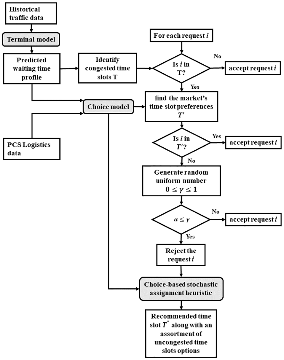
Components of the proposed time slot management system (TSMS).

As can be seen in Figure 1, this framework requires three models. The first model is a terminal model to simulate the processes at the terminal gates and predict the waiting time profile. The second is a choice model to gain insight into the preferences of the TOC about the container pick-up times. Finally, the third model is a truck shifting heuristic that recommends an alternative time slot to a portion of trucks based on an application rate α. The next paragraphs explain the method used to develop each component as well as the data used for a case study in the port of Rotterdam.

Traffic and Logistic Data

The data that has been collected for the methodology is twofold. The first data source is historic traffic data from 2017 collected from loop detectors located at the terminal gates. This data captures the number of trucks that arrive at the terminal per time of the day. The truck arrivals are aggregated by the data provider and therefore are available every 1 h. The second data source is historic logistic data from 2017, collected from the PCS in the port of Rotterdam. The logistic data captures details of import containers. This is revealed preference data of TOC for container pick up. The data set contains information of transaction data for the arrival of container vessels, container discharges, and the estimated pick-up time of these containers by hinterland transport trucks. Moreover, the data set includes container characteristics and information about the transported commodity. Additionally, the waiting time at the terminals obtained from the terminal model is included in the logistic data set.

Terminal Model

The terminal model is formulated as an M/M/s queueing model which the notation instances for a multi-server model with Poisson arrivals and exponential service times. The terminal model includes three components, that is, the truck generator, trucks, and a server. Together, these three components make up three processes in the terminal model. The three processes in the model are the arrival process, the server process, and the departure process. Figure 2 provides a graphical overview of the terminal model.

Figure 2.

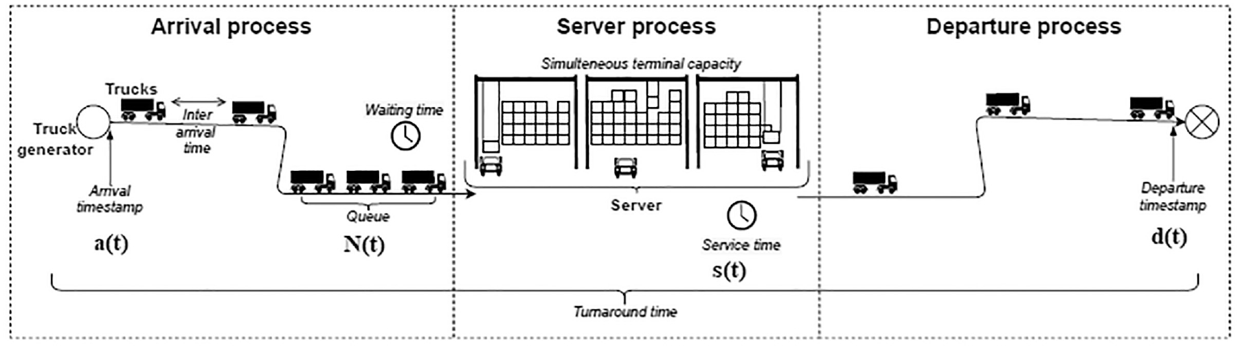
Graphical representation of the terminal model.

Equation 1 simply calculates the queue length per unit of time which is the number of the truck arrivals minus the trucks being served and the trucks that have departed.

$$N(t)=a(t)-s(t)-d(t)$$

(1)

It is assumed that both the inter-arrival time and the service time are independent and identically distributed random variables with an exponential distribution, and gates serve trucks with an integer number of cranes, that is, servers. For the arrival process, a non-stationary arrival profile is used, as the inter-arrival time between trucks is different for each hour of the day (i.e., IAT_h in min). The historic traffic data from loop detectors at terminal gates contains the average number of trucks arriving for each hour of the day (λ_h). Equation 2 presents the inter-arrival time:

$$\mathrm{IA}{T}_h=\exp \left(\frac{60}{{\lambda }_h}\right)$$

(2)

The mathematical foundation for calculating waiting time is based on Little’s law and is presented in Equations 3 to 5.

$$L={\lambda }_{h}W$$

(3)

$$L_q={\lambda }_h{W}_q$$

(4)

$$W=W_q+\mu$$

(5)

where

L = expected number of trucks in the queueing system including trucks that are waiting in the queue and trucks that are loading a container in the servers,

λ _h = mean arrival rate for each hour,

W = waiting time including service time (min),

μ = mean service time (min) which is from an exponential distribution,

L_q = expected queue length, and

W_q = waiting time in the queue (min).

To set up the queue model of a terminal, the mean service time μ and the number of servers (simultaneous terminal capacity) have to be known. In this case study, this information is missing. Therefore, these two parameters are estimated by iterative examination of different settings for the queue simulation while minimizing the mean squared differences between the simulated (Y) and observed ( $\hat{Y}$ ) departure profiles (Equation 6). Bayesian optimization is used, which is a simulation-based optimization algorithm that seeks the global minimum with a few numbers of the simulation run.

$$\mathrm{MSE}=\frac{1}{n}\sum _{i=1}^n(Y_i-{\hat{Y}}_i{)}^2$$

(6)

Choice Model

The model used in this study is a multinomial logit model. This model is defined to understand the choice of a TOC to pick up a certain container at a certain time. The probability of choosing a certain time P(t|T) is computed from the attractiveness of the alternatives. The attractiveness is measured by the utility maximization theory. In this theory, the alternative with the highest utility is always chosen (Equation 7),

$$P(t|T)=P(U_t\ge U_j,\forall j\in T)$$

(7)

However, it is impossible to capture all factors in the choice model that influence the choice. The utility function U_t, therefore, consists of two parts (Equation 8),

$$U_t=V_t+{\epsilon }_t$$

(8)

where

V_t = the first is the deterministic part of the utility, which includes the attributes that are found to influence the choice of a certain alternative,

ε_t = an error term contained in the second part of the utility function. This error term represents the unobserved behavior that influences the choice.

The deterministic part of the utility function can also capture the unobserved behavior of the decision-maker through an alternative specific constant (ASC).

The alternatives in the model are times of the day which are aggregated into four periods. The periods are formulated as night (from 00:00 to 04:00 and from 21:00 to 00:00), morning (from 04:00 to 10:00), midday (from 10:00 to 15:00), and afternoon (from 15:00 to 21:00). These periods are based on observed arrival patterns and time slot categories used in practice at the terminals.

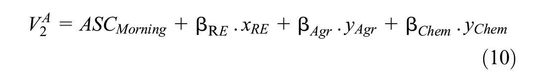
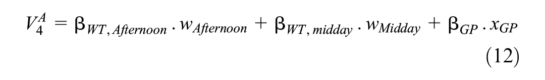
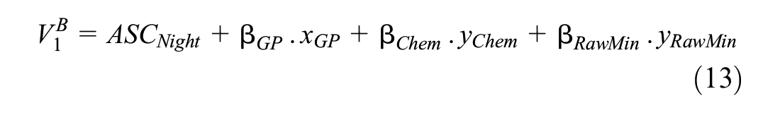
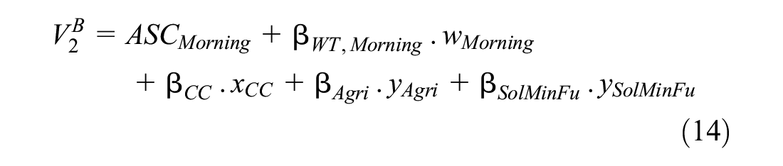
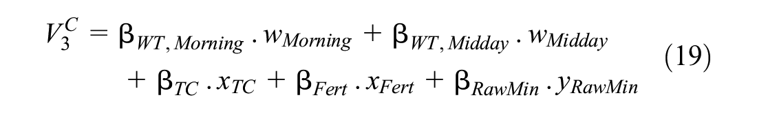
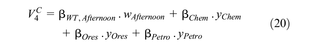
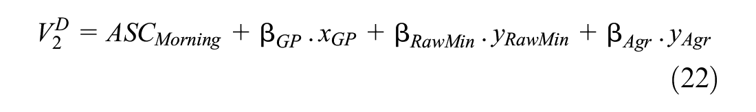
Since the distribution of containers and commodities differs between terminals, a separate choice model is defined for each terminal; therefore a separate set of utility functions is formulated. The observed behavior in the utility for a certain alternative is captured by the independent variables in the deterministic part of the utility V_t. Note that V₁ represents the night, V₂ the morning, V₃ the midday, and V₄ the afternoon. The independent variables considered in the model are container type (x_type), commodity type (y_type), and waiting time per alternative (w_alt). The waiting time is simulated with the terminal model. It is assumed that a TOC has some perception about the waiting time at gates at different times of the day that may influence its arrival time choice.

The ASCs for the night and morning alternatives are formulated to capture the unobserved factors that decrease the preference for these two alternatives (ASC_alt). The model specifications are presented in Equations 9 to 24. The subscripts are defined in the result section in Table 3.

Terminal A:

$$V_1^A=\mathrm{AS}{C}_{\mathrm{Night}}+{\beta }_{\mathrm{R}E}.x_{\mathrm{RE}}+{\beta }_{\mathrm{SolMinFu}}.y_{\mathrm{SolMinFu}}$$

(9)

$$V_2^A=\mathrm{AS}{C}_{\mathrm{Morning}}+{\beta }_{\mathrm{R}E}.x_{\mathrm{RE}}+{\beta }_{\mathrm{Agr}}.y_{\mathrm{Agr}}+{\beta }_{\mathrm{Chem}}.y_{\mathrm{Chem}}$$

(10)

$$V_3^A={\beta }_{\mathrm{WT},\mathrm{Morning}}.w_{\mathrm{Morning}}+{\beta }_{\mathrm{TC}}.x_{\mathrm{TC}}+{\beta }_{\mathrm{CC}}.x_{\mathrm{CC}}$$

(11)

$$V_4^A={\beta }_{\mathrm{WT},\mathrm{Afternoon}}.w_{\mathrm{Afternoon}}+{\beta }_{\mathrm{WT},\mathrm{midday}}.w_{\mathrm{Midday}}+{\beta }_{\mathrm{GP}}.x_{\mathrm{GP}}$$

(12)

Terminal B:

$$V_1^B=\mathrm{AS}{C}_{\mathrm{Night}}+{\beta }_{\mathrm{GP}}.x_{\mathrm{GP}}+{\beta }_{\mathrm{Chem}}.y_{\mathrm{Chem}}+{\beta }_{\mathrm{RawMin}}.y_{\mathrm{RawMin}}$$

(13)

$$\begin{array}{c}\multicolumn{1}{c}{V_2^B=\mathrm{AS}{C}_{\mathrm{Morning}}+{\beta }_{\mathrm{WT},\mathrm{Morning}}.w_{\mathrm{Morning}}}\\ \multicolumn{1}{c}{+{\beta }_{\mathrm{CC}}.x_{\mathrm{CC}}+{\beta }_{\mathrm{Agri}}.y_{\mathrm{Agri}}+{\beta }_{\mathrm{SolMinFu}}.y_{\mathrm{SolMinFu}}}\end{array}$$

(14)

$$V_3^B={\beta }_{\mathrm{WT},\mathrm{Midday}}.w_{\mathrm{Midday}}+{\beta }_{\mathrm{WT},\mathrm{Afternoon}}.w_{\mathrm{Afternoon}}$$

(15)

$$V_4^B={\beta }_{\mathrm{RE}}.x_{\mathrm{RE}}+{\beta }_{\mathrm{Petro}}.y_{\mathrm{Petro}}$$

(16)

Terminal C:

$$V_1^C=\mathrm{AS}{C}_{\mathrm{Night}}+{\beta }_{\mathrm{GP}}.x_{\mathrm{GP}}+{\beta }_{\mathrm{CC}}.x_{\mathrm{CC}}+{\beta }_{\mathrm{TC}}.x_{\mathrm{TC}}$$

(17)

$$V_2^C=\mathrm{AS}{C}_{\mathrm{Morning}}+{\beta }_{\mathrm{R}E}.x_{\mathrm{RE}}+{\beta }_{\mathrm{SolMinFu}}.y_{\mathrm{SolMinFu}}$$

(18)

$$\begin{array}{c}\multicolumn{1}{c}{V_3^C={\beta }_{\mathrm{WT},\mathrm{Morning}}.w_{\mathrm{Morning}}+{\beta }_{\mathrm{WT},\mathrm{Midday}}.w_{\mathrm{Midday}}}\\ \multicolumn{1}{c}{+{\beta }_{\mathrm{TC}}.x_{\mathrm{TC}}+{\beta }_{\mathrm{Fert}}.x_{\mathrm{Fert}}+{\beta }_{\mathrm{RawMin}}.y_{\mathrm{RawMin}}}\end{array}$$

(19)

$$\begin{array}{c}\multicolumn{1}{c}{V_4^C={\beta }_{\mathrm{WT},\mathrm{Afternoon}}.w_{\mathrm{Afternoon}}+{\beta }_{\mathrm{Chem}}.y_{\mathrm{Chem}}}\\ \multicolumn{1}{c}{+{\beta }_{\mathrm{Ores}}.y_{\mathrm{Ores}}+{\beta }_{\mathrm{Petro}}.y_{\mathrm{Petro}}}\end{array}$$

(20)

Terminal D:

$$V_1^D=\mathrm{AS}{C}_{\mathrm{Night}}+{\beta }_{\mathrm{CC}}.x_{\mathrm{CC}}+{\beta }_{\mathrm{Chem}}.y_{\mathrm{Chem}}$$

(21)

$$V_2^D=\mathrm{AS}{C}_{\mathrm{Morning}}+{\beta }_{\mathrm{GP}}.x_{\mathrm{GP}}+{\beta }_{\mathrm{RawMin}}.y_{\mathrm{RawMin}}+{\beta }_{\mathrm{Agr}}.y_{\mathrm{Agr}}$$

(22)

$$V_3^D={\beta }_{\mathrm{SolMinFu}}.y_{\mathrm{SolMinFu}}+{\beta }_{\mathrm{Petro}}.y_{\mathrm{Petro}}$$

(23)

$$\begin{array}{c}\multicolumn{1}{c}{V_4^D={\beta }_{\mathrm{WT},\mathrm{Midday}}.w_{\mathrm{Midday}}+{\beta }_{\mathrm{CC}}.x_{\mathrm{CC}}}\\ \multicolumn{1}{c}{+{\beta }_{\mathrm{SolMinFu}}.y_{\mathrm{SolMinFu}}+{\beta }_{\mathrm{Ores}}.y_{\mathrm{Ores}}}\end{array}$$

(24)

The parameters can be estimated using the maximum log-likelihood estimation. The maximum likelihood is the probability that the model correctly fits the observations from data. In the maximum log-likelihood estimation, the model aims to estimate the parameters such that the model has the highest probability of fitting the observed data. Equation 25 presents the maximum log-likelihood function

$$maxL({\hat{\beta }}_1,...,{\hat{\beta }}_k)=\sum _{n=1}^N(\sum _{t\in T_n}{y}_{\mathrm{tn}}\ln P_n(t\in T_n|x,y,w),$$

(25)

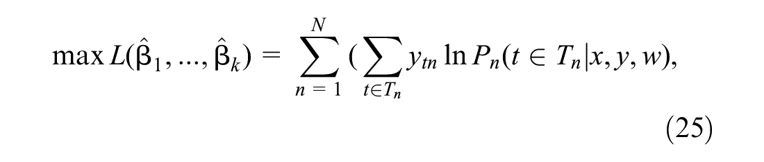
where L = the log-likelihood.

If a TOC chooses alternative t, y_tn = 1 and 0 otherwise. P_n(t|T_n) represents the probability that a TOC n chooses alternative t from the choice set T_n (Equation 26).

$$P(t\in T_n|x,y,w)=\frac{e^{V_{\mathrm{tn}}}}{\sum _{j\in T_n}{e}^{V_{\mathrm{jn}}}},$$

(26)

To judge the performance and accuracy of the choice model, the goodness of fit, t-values, and p-values are used. The goodness of fit can be observed from the likelihood ratio (Equation 27)

$$-2(L(0)-L(\hat{\beta }))$$

(27)

The likelihood ratio compares a model where all parameters are set to zero L(0) with the model with the estimated parameter L( $\hat{\beta }$ ). The likelihood ratio statistic indicates whether the estimated model is significantly better than the model with equal probabilities. The t-value is calculated by Equation 28

$$t_k=\frac{{\hat{\beta }}_k}{{\sigma }_k}$$

(28)

where

$\hat{\beta }$ = the estimated parameter, and

σ = the standard error of the parameter.

Then, the p-value can be computed by Equation 29.

$$p_k=2(1-\Phi (t_k))$$

(29)

where Ф = the cumulative density function of the univariate standard normal distribution.

The next section shows how the choice model is used in the truck shifting heuristic.

Choice-Based Stochastic Assignment

The method explained here is the choice-based stochastic assignment illustrated in Figure 1. It is assumed that the trucks whose requests are rejected all accept the recommended alternative from the system. This is because the desired outcome is to estimate the maximum expected total gain in the planning horizon after the implementation of the system. To this end, the truck shifting heuristic has to compute new arrival profiles based on the truck shifting strategies that result from the choice models. This process is explained in four steps as follows:

• 1) Convert containers to trucks: First of all, a comparison between the logistic data and traffic data is used to convert the number of containers to the number of trucks. From the logistic data of import containers, occurrence probability percentages for container and commodity types are obtained for each period. This makes it possible to calculate an absolute number of trucks transporting a specific container or commodity per time interval.

• 2) Temporal distribution matrix: The temporal distribution of commodity or container type along a day is presented in the form of a matrix N_T×C with rows representing choice alternatives T = {1, 2, 3 ,t} and columns representing container and commodity types C = {1, 2, 3,…c}. see Equation 30.

$$N_{T\times C}=\left(\begin{array}{ccc}{N}_{11}\hfill & \dots \hfill & N_{1c}\hfill \\ \multicolumn{1}{c}{⋮}& \ddots \hfill & ⋮\hfill \\ \multicolumn{1}{c}{N_{t1}}& \cdots \hfill & N_{\mathrm{tc}}\hfill \end{array}\right)\forall t\in T,c\in C$$

(30)

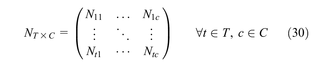
where N_tc = the number of trucks that requested to pick up a certain container or commodity c at period t.

• 3) Find the recommended alternative: the desired outcome is to find the best alternative time slot j which has a minimum deviation from the requested time slot i and also has the highest attractiveness for the container or commodity type c. The system finds this alternative time slot by solving the optimization problem in Equation 31:

$$min\sum _{c\in C}\sum _{i\in T}\sum _{j\in T}|i-j|N_{\mathrm{ic}}\alpha (1-P(j|c,w_j)x_{\mathrm{ij}}^c$$

(31)

where

$x_{\mathrm{ij}}^c$ = a binary decision variable equal to 1 if trucks with container/commodity type c are shifted from their requested time slot i to the alternative time slot j, and 0 otherwise,

P(j|c,w_j) = the estimated choice probability of time slot j given the commodity or container type c and waiting time w_j. (This probability comes from the choice model [Equation 26]),

N_ic = the number of trucks that have requested to pick up container c at time slot i (Equation 30), and

α = the application rate that will be defined by policymakers (Figure 1) and is used as a knob to do policy assessment analysis in this paper.

• 4) Arrival profile reconstruction: The solution of the above optimization problem is used to calculate the new arrival profile for each application rate. The new arrival profile is then used as the input to the terminal model to calculate the new waiting time profile. This waiting time can be used to evaluate the gain from the application of the proposed TSMS.

Waiting Time Gain Calculation

The waiting profile represents the average waiting time for one truck in each hour. The waiting time gain can be calculated by comparing the total waiting time after the application of the proposed TSMS with the base case profile. The total waiting time gain for the entire day indicates the impact of TSMS under a certain application rate.

Results

This section describes calibration and validation results for the terminal model, the preferences of TOC based on the choice model, and the expected waiting for time gains and monetary gains when TSMS is applied to the terminals in the Port of Rotterdam.

Terminal Model Calibration

To ensure that the terminal models are close to reality, each terminal model has been calibrated by tuning the arrival and service process parameters for each terminal based on the historically observed arrival and departure profile. Data for 12 months in 2017 has been collected and this data has been divided into two calibration and validation datasets: the calibration dataset includes 11 months to calculate the average working day profile, since the statistical tests, for example, ANOVA and two-sided t-test, showed that there are no significant monthly or daily trends that must be accounted for in arrival or departure profiles. The one drop-out month then is used as a validation set to calculate the average arrival and departure profile for validation of the model.

Arrival Process

The parameter λ_h in Equation 2 has been calibrated for the arrival process based on the arrival profile from historic traffic data. The tuned parameters have been used in the terminal model to simulate the arrival process as discussed above. A two-sided t-test showed that there is a significant similarity between the observed and simulated arrival profile.

Service Process

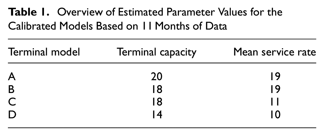
For the service process, the number of servers and the mean service time have been calibrated. The historic departure profile is used to tune the parameters. Similar to the arrival process, a two-sided t-test has been applied to compare the observed and simulated departure profiles. Moreover, polynomial regression has been used to test the correlation between the observed and simulated arrival profile. The results show that all the terminal models can accurately predict truck departure flow with p-values < 0.05, and correlation coefficients > 0.93. The calibrated parameter of each terminal model is presented in Table 1.

Table 1.

Overview of Estimated Parameter Values for the Calibrated Models Based on 11 Months of Data

Terminal model	Terminal capacity	Mean service rate
A	20	19
B	18	19
C	18	11
D	14	10

Terminal Model Validation

The terminal model has been validated using a test set. By splitting the historic traffic data set into two parts, the train set and test set are created. The train set comprehends traffic data of 11 months of the year. The test set includes the data of the remaining month. The calibrated model has been validated using the test data set (Figure 3). This test set allows for an unbiased evaluation of the model. The statistical tests and polynomial regression show that the model can predict the unseen departure profiles with high accuracy (with a correlation coefficient of >0.91).

Figure 3.

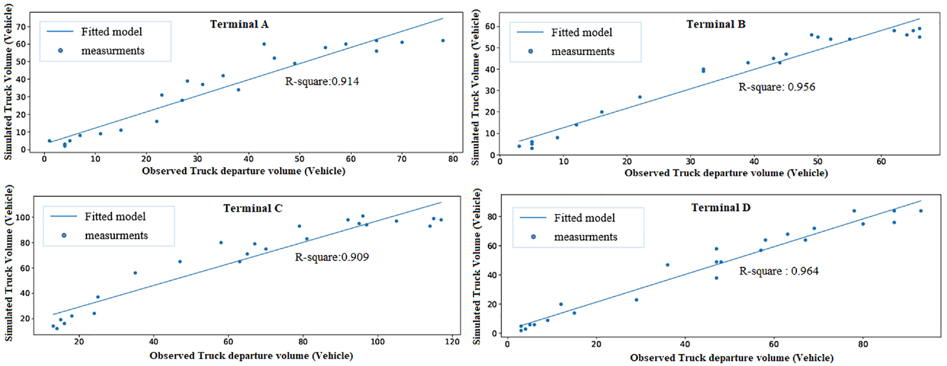
Average observed and simulated departure profiles.

Truck Operating Companies’ (TOCs)’s Preferences

The results from the arrival time choice model are depicted in Table 2. As opposed to the container and commodity type variables, the waiting time is a continuous variable and its parameter can show the effect of one minute waiting time extra on the utility. In general, the impact of waiting time on the pick-up time choice of TOCs is relatively small. However, the TOCs seem to value morning waiting times more than midday and afternoon waiting times. For terminals B and C, the waiting time impacts in the midday and afternoon are noticeable. One minute of waiting time in the midday and afternoon is more important for these two terminals as compared with terminals A and D. Note that the morning waiting time parameter is positive. This means that, if the waiting time in the morning increases, the preferences of TOCs for the morning period also increase. This counterintuitive result could be because of some latent attitude of TOCs, for example, arrival of large vessels in the morning.

Table 2.

Results of the Pick-Up Time Choice Models

Parameters	Terminal A, LR = 13,326.87			Terminal B, LR = 26,640.73			Terminal C, LR = 46,274.5			Terminal D, LR = 118,682.2
	Estimate	t	p	Estimate	t	p	Estimate	t	p	Estimate	t	p
$\mathrm{AS}{C}_{\mathrm{Night}}$	−1.52	−78.9	0	−2.13	−75	0	−2.01	−50.4	0	−1.68	−244	0
$\mathrm{AS}{C}_{\mathrm{Morning}}$	−0.601	−36.2	0	−0.407	−33.9	0	−0.338	−40.4	0	−0.333	−46.2	0
${\beta }_{\mathrm{GP}}$	−0.265	−15.1	0	0.325	10.2	0	0.245	5.89	0	−0.107	−13.2	0
${\beta }_{\mathrm{RE}}$	0.288	15.6	0	−0.906	−37.4	0	0.418	14.7	0	na	na
${\beta }_{\mathrm{CC}}$	0.187	6.01	0	−0.096	−4.67	0	0.196	3.31	0.00	−0.0374	−4.28	0
${\beta }_{\mathrm{TC}}$	0.0855	2.83	0.00	na	na	0	0.0801	3.24	0.00	na	na
${\beta }_{\mathrm{Arg}}$	0.177	5.57	0	0.548	14.6	0	0.344	11.7	0	0.322	21.3	0
${\beta }_{\mathrm{Chem}}$	0.27	5.64	0	0.287	5.61	0	0.124	9.31	0	0.265	17.9	0
${\beta }_{\mathrm{SolMinFu}}$	1.18	26.1	0	0.0967	2.29	0.02	0.297	16.8	0	−0.088	−7.66	0
${\beta }_{\mathrm{RawMin}}$	na	na	na	0.333	4.48	0	−0.217	−9.77	0	−0.0569	−3.91	0
${\beta }_{\mathrm{Petro}}$	na	na	na	0.175	4.2	0	0.134	7.26	0	0.0532	4.37	0
${\beta }_{\mathrm{Ores}}$	na	na	na	na	na	na	0.108	4.87	0	−0.0378	−2.78	0.00
${\beta }_{\mathrm{Fert}}$	na	na	na	na	na	na	−0.0656	−2.94	0.00	na	na	na
${\beta }_{\mathrm{WT},\mathrm{Morning}}$	0.079	2.36	0.01	0.0688	2.25	0.02	−0.173	−2.93	0.00	na	na	na
${\beta }_{\mathrm{WT},\mathrm{Midday}}$	−0.00386	−3.01	0.00	−0.0222	−13.7	0	−0.0173	−8.94	0	−0.0139	−8.17	0
${\beta }_{\mathrm{WT},\mathrm{Afternoon}}$	−0.00193	−2.24	0.02	−0.0177	−15.5	0	0.00806	14.8	0	na	na	na

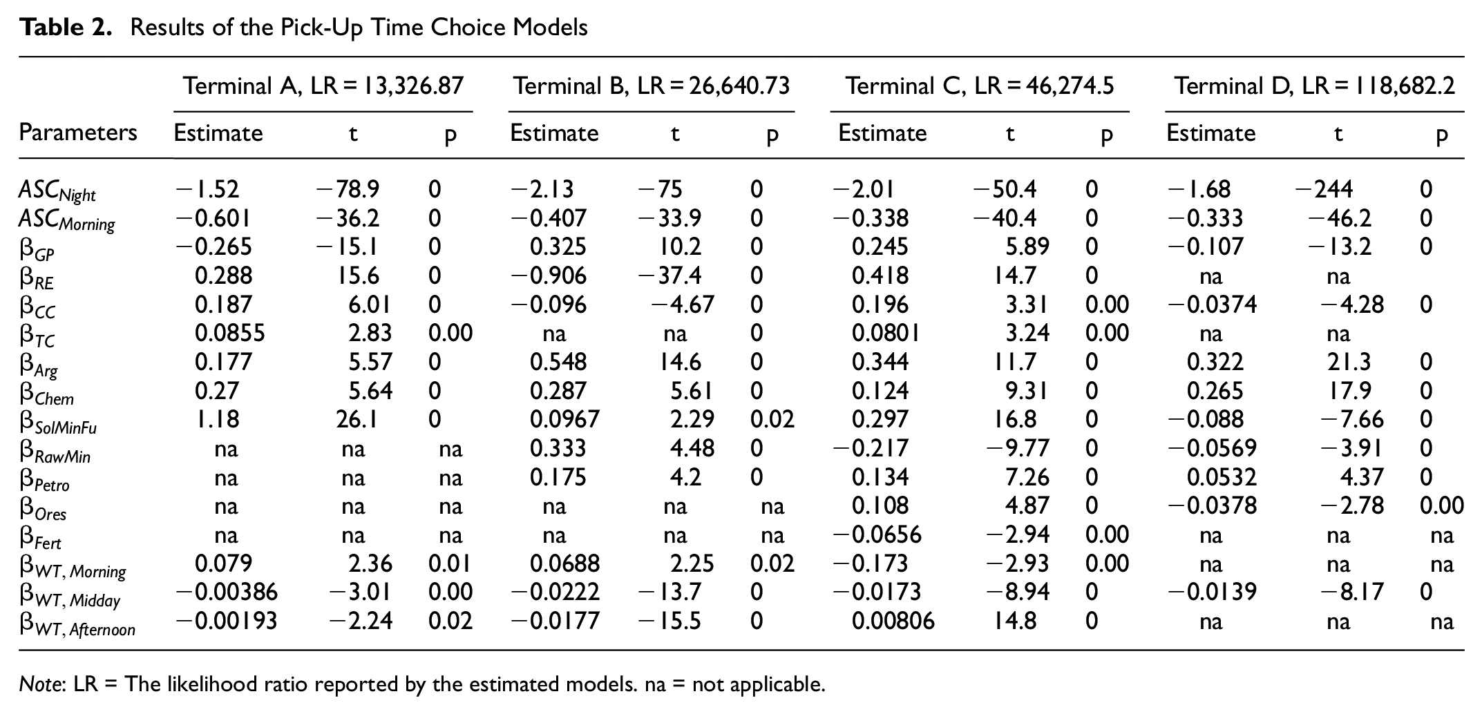
Note: LR = The likelihood ratio reported by the estimated models. na = not applicable.

Concerning the contextual variables, that is, commodity and container types, the sign and magnitude of the parameters have been used to derive the preferences of the transport markets toward an alternative time slot for container pick-ups. These preferences are summarized in Table 3. This indicates that truckers’ preferences of pick-up time windows can be characterized by the commodity and container type. For example, it can be seen that containers that contain agricultural products have preferences toward morning pick-up. Reefer containers are more likely to be picked up in the night or morning. TSMS uses these preferences to assign trucks to their preferred time windows if their requested time slot is rejected because of congestion.

Table 3.

Preferences of Truck Operating Companies (TOCs) Based on the Container or Commodity Type

Terminals	Market	Pick-up period preferences and disinclinations
		Night (00:00-04:00) (21:00-00:00)	Morning (04:00-10:00)	Midday (10:00-15:00)	Afternoon (15:00-21:00)
A	General-purpose container (GP)	+	+	+	-
	Reefer container (RE)	+	+	-	-
	Chemical container (Chem)	-	-	+	-
	Tank container (TC)	-	-	+	-
	Agricultural products (Agr)	-	+	-	-
	Chemical products (Chem)	-	+	-	-
	Solid mineral fuels (SolMinFu)	+	-	-	-
B	General-purpose container (GP)	+	-	-	-
	Reefer container (RE)	+	+	+	-
	Chemical container (Chem)	+	-	+	+
	Agricultural products (Agr)	-	+	-	-
	Chemical products (Chem)	+	-	-	-
	Solid mineral fuels (SolMinFu)	-	+	-	-
	Raw minerals (RawMin)	+	-	-	-
	Petroleum (Petro)	-	-	-	+
C	General-purpose containers (GP)	+	-	-	-
	Reefer containers (RE)	-	+	-	-
	Chemical containers (Chem)	+	-	-	-
	Tank containers (TC)	+	-	+	-
	Agricultural products (Agr)	-	+	-	-
	Chemical products (Chem)	-	-	-	+
	Solid mineral fuels (SolMinFu)	-	+	-	-
	Raw minerals (RawMin)	+	+	-	+
	Petroleum (Petro)	+	-	-	+
	Ores	-	-	-	+
	Fertilizers (Fert)	+	+	-	+
D	General-purpose container (GP)	+	-	+	+
	Chemical container (Chem)	-	+	+	-
	Agricultural products (Agr)	-	+	-	-
	Chemical products (Chem)	+	-	-	-
	Solid mineral fuels (SoMinFu)	+	+	-	-
	Raw minerals (RawMin)	+	-	+	+
	Petroleum (Petro)	-	-	+	-
	Ores	+	+	+	-

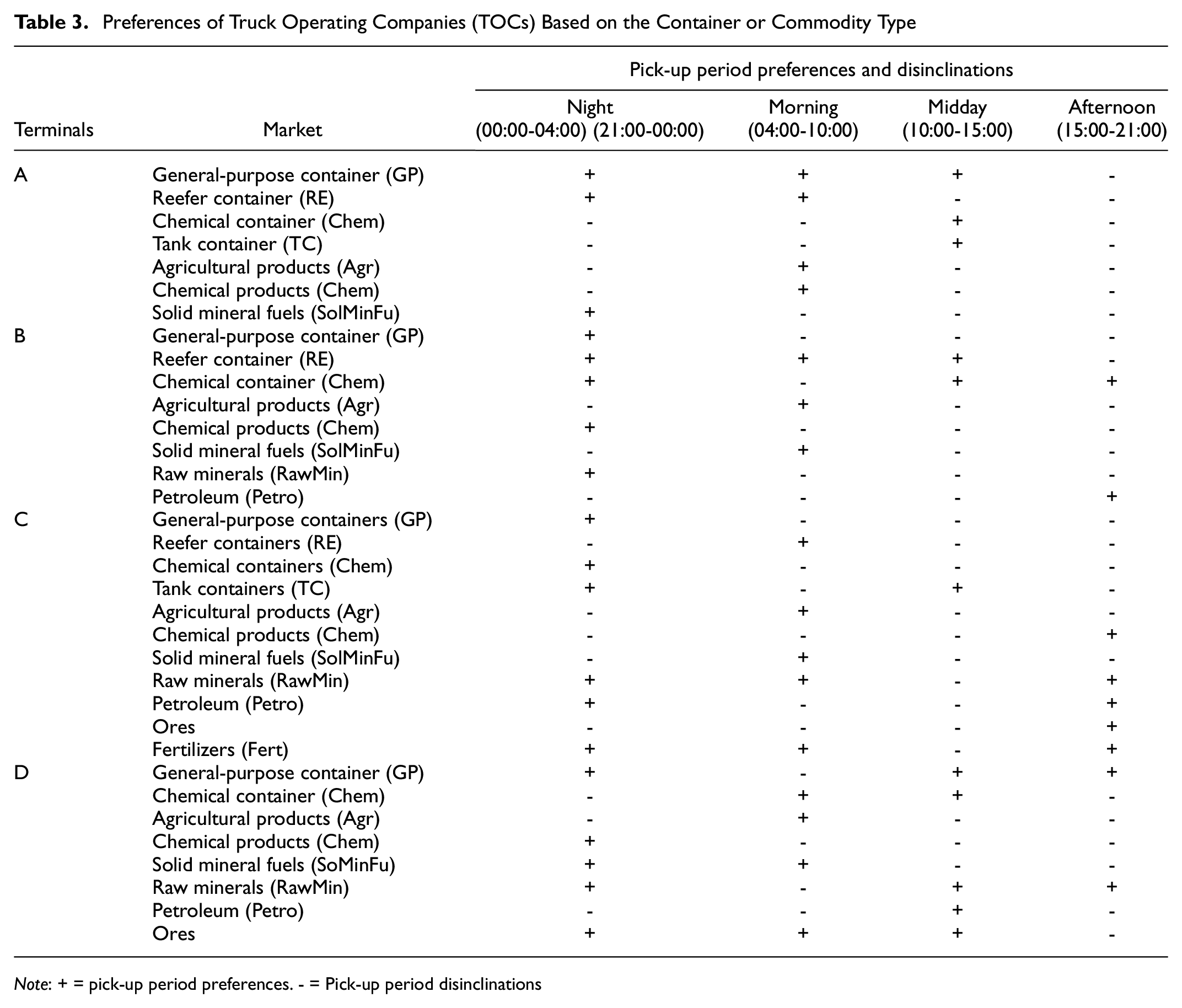
Note: + = pick-up period preferences. - = Pick-up period disinclinations

Total Gains

This section defines various scenarios to evaluate the effect of the proposed TSMS under various TOC application rates. In scenarios 1 to 10, the application rate (α) changes from 5% to 50%, with a step size of 5%. In scenarios 11 to 15, α changes from 60% to 100%, with a step size of 10%. The results are compared with a reference scenario in which an entirely equal spread of trucks along the day is simulated. For each designed scenario, the TSMS can generate new simulated arrival and departure profiles and the corresponding waiting time profiles. Comparing the simulated waiting time profiles with the base case provides insight into the effect of the TSMS on the waiting time. This helps to realize both the gain and drawbacks of TSMS. Note that when too many trucks are shifted away from the peak, a new peak might occur during other periods. This will cause waiting time in other periods. The total waiting time gain provides insight into how effectively the system works. The development of waiting time gains under various application rates (scenarios) is displayed in Figure 4. The x-axis on the graphs shows the application rate α and the y-axis is the waiting time gain in hour.

Figure 4.

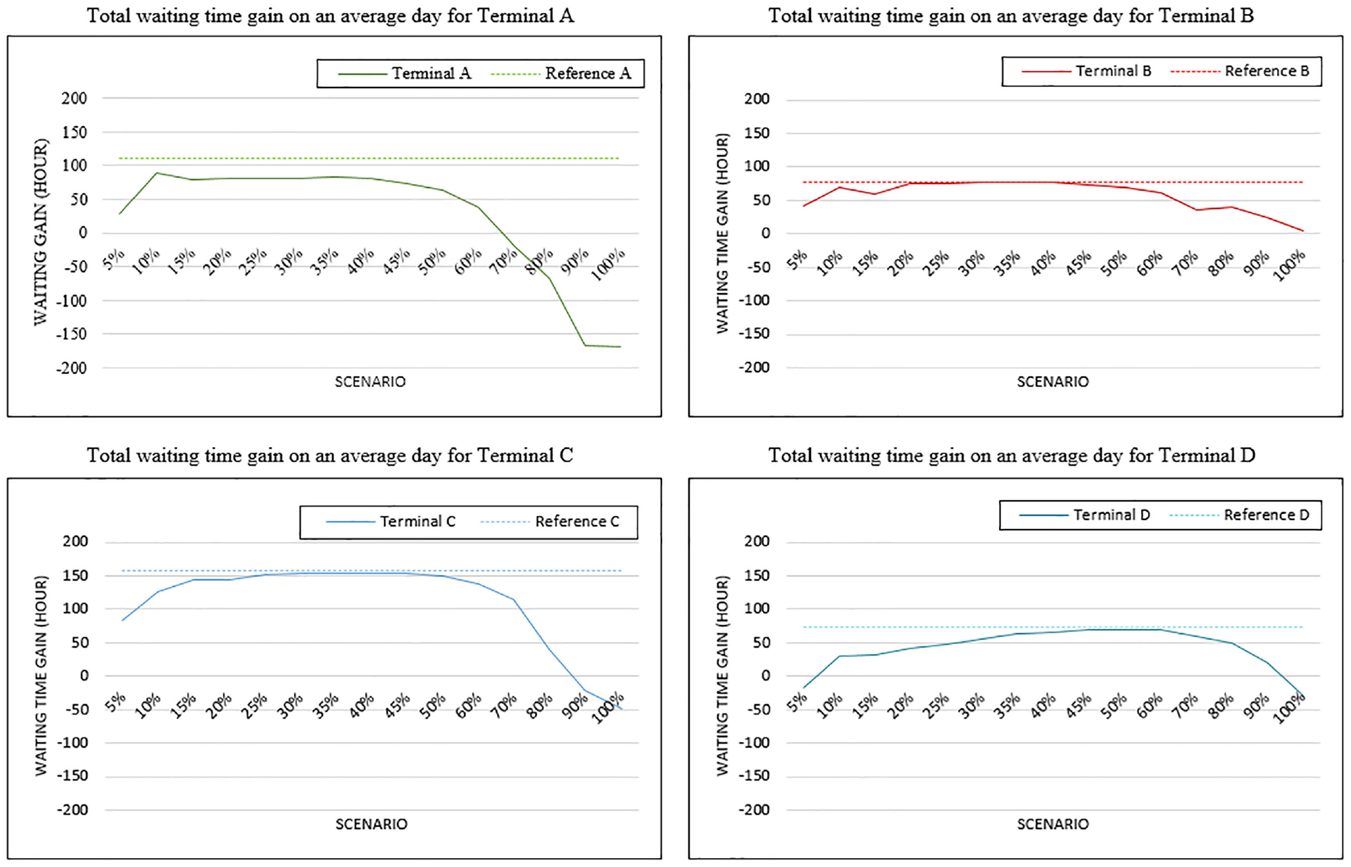
Total waiting time gains for the proposed time slot management system (TSMS).

The solid lines represent the development of the waiting time gains under various application rate scenarios. The dotted lines represent the waiting time gain for the reference scenario. Please note that in the reference case the number of trucks arriving will always stay below the terminal capacity and there will not be any waiting time. Consequently, the waiting time gain in the reference scenario is the largest gain possible. From Figure 4 it can be observed that there is no linear relation between application rates and waiting time gain. An increase of 5% for shifting trucks does not cause a 5% increase in waiting time gain. For most terminals, an increase of the waiting time gain can be observed from the first scenario (5% shift) until the seventh scenario (35% shift). Thereafter, for each terminal, the waiting time gain decreases and eventually becomes negative for some terminals. This insight indicates that there is an optimum setting for time slot management to reduce waiting times. Additionally, it is observed that the gain with small application rates (5%–10%) is already very close to this optimum (see Figure 5). The optimum waiting time gain would be achieved with a shift of around 40% of truck arrivals. It can be seen from Figure 5, in all terminals except terminal D, that a 10% application rate would lead to a significant reduction in waiting time. This proves that TSMS can successfully mitigate congestion at terminal gates by minimum changes in the pick-up time of the containers.

Figure 5.

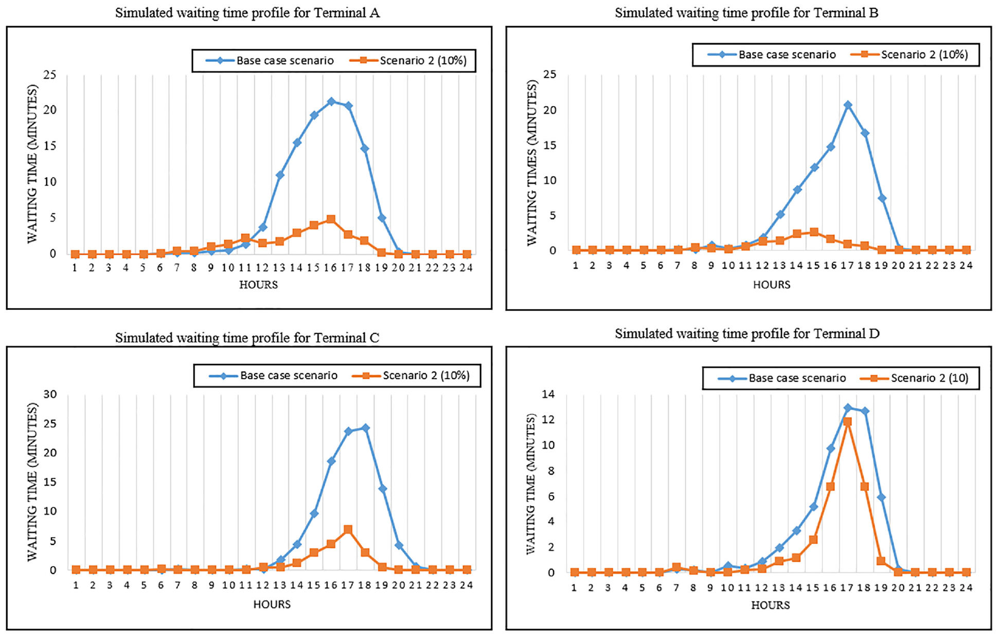
The waiting time reduction per terminal for α = 10%.

Monetary Gain

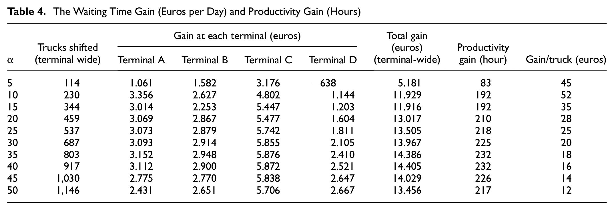
Hourly waiting time gains are difficult to interpret for the entire system as it is not immediately clear what 1 h of waiting time gain means and for who this gain is beneficial. For the interpretation of the results, the waiting time gains in hours are converted to monetary values (euro). In the year 2017, the reported cost for transporting a container was approximated to 62 euros per hour in the Netherlands. The waiting cost in container transport was estimated at around 38 euros per hour. In Table 4, the waiting time gain in hours is converted to a monetary gain in euro and a productivity gain in hours for TOCs. The monetary gain indicates the cost saved by the TOC because of less waiting time at the terminal. The productivity gain in Table 4 represents the extra hours that carriers can be on roads transporting containers if not waiting at the terminal gates. This is calculated by dividing the total waiting time gain (terminal-wide) by the cost of transporting a container on the road (62 euros per hour). This proves that implementation of the TSMS allows for around 192 h of productivity gain per day. In other words, the waiting time gain for TOCs equals the transportation of around 192 containers for 1 h. This can add 10% efficiency to container road transport. In Table 4, the terminal-wide total gain is reported. This is the amount of gain for all the trucks in the system and can also be referred to as social gain. The “gain/truck” is the average contribution of a shift made by one single truck to the entire system. The numbers show that a shifting percentage of 10% will provide the highest value (52 euros) in relation to effort and reward.

Table 4.

The Waiting Time Gain (Euros per Day) and Productivity Gain (Hours)

α	Trucks shifted (terminal wide)	Gain at each terminal (euros)				Total gain (euros) (terminal-wide)	Productivity gain (hour)	Gain/truck (euros)
		Terminal A	Terminal B	Terminal C	Terminal D
5	114	1.061	1.582	3.176	−638	5.181	83	45
10	230	3.356	2.627	4.802	1.144	11.929	192	52
15	344	3.014	2.253	5.447	1.203	11.916	192	35
20	459	3.069	2.867	5.477	1.604	13.017	210	28
25	537	3.073	2.879	5.742	1.811	13.505	218	25
30	687	3.093	2.914	5.855	2.105	13.967	225	20
35	803	3.152	2.948	5.876	2.410	14.386	232	18
40	917	3.112	2.900	5.872	2.521	14.405	232	16
45	1,030	2.775	2.770	5.838	2.647	14.029	226	14
50	1,146	2.431	2.651	5.706	2.667	13.456	217	12

Discussion

To assess the ability as well as the limitations of the proposed TSMS at terminal gates, the findings are summarized and discussed in this section. This research shows that it is possible to utilize traffic and logistics data to extract valuable knowledge about TOCs preferences and use this knowledge to control traffic at terminal gates. This approach considers two main actors from two sides of the system; that is, terminals at port and TOC in the hinterland. However, there are more stakeholders in the system—such as public sectors, shippers, forwarders, warehouses, and so forth—whose decisions may have a significant impact on terminal (or hinterland) congestion and whose costs arising from either terminal operations or the proposed time-slot interventions are relevant in assessing efficacy. This collective perspective could be captured by applying a multi-stakeholder analysis and could help to investigate other costs and benefits in the system such as emission reduction gains associated with congestion reduction at gates.

The proposed system maximizes the waiting time gain. However, ideally the effort to shift (e.g., tour re-planning costs) should also be considered. Therefore, the optimum waiting time gain achieved by a 35%–45% shift percentage might not reflect the ideal situation for shifting trucks. In this research, this impact was limited by fine-tuning the application rate so that the minimum number of shifts would lead to the maximum amount of gain. Moreover, the costs of shifting to another time are directly experienced by a TOC, whereas the benefits from the control system will only indirectly reach them (if at all). Policymakers can consider giving some extra incentives by sharing information, giving priority, or reducing the chance of being rejected in their next calls. Decision-makers can also consider compensating truckers’ effort by recycling a part of public monetary gains (e.g., emission gains) to the shifted trucks.

From the application perspective, the advisory-based TSMS not only proved its ability to mitigate waiting times at terminal gates but also proved to be a great policy assessment and decision support tool for decision-makers. It helps them to turn data to value, get insights about the behavior of truckers, and ease integrated traffic and logistics management at logistic hubs.

Conclusions

In this paper, an advisory-based TSMS has been presented. The novelty of this research is that it proposes a new modeling framework that can be used to design more efficient TSMSs considering both the port and hinterland side in the design of a truck appointment system which can be used to reduce truck waiting times at terminals. The method combines a queueing model to simulate the processes at terminals and integrates choice modeling with optimization to control truck arrivals at the terminals taking the preferences of truckers into account. An application of the TSMS to the terminals in the Port of Rotterdam showed that by rescheduling a small portion of trucks, remarkable waiting time gains and productivity gains can be achieved. The key findings from this research are as follows:

• The proposed TSMS can save up to 1,2000 euros per day by shifting only 10% of truck schedules.

• This system allows for 192 extra hours of productivity which can add to the benefits of trucking companies and increase the efficiency of road container transport by 10%.

• Truckers can be prioritized for each time-window based on their market preferences. For example, containers carrying agricultural products have a preference for morning pick-ups, and reefer containers have preferences for night and morning pick-ups.

With respect to future research, the authors recommend including internal operations in the terminal model, including vessel arrivals, in the TOC choice models, and coupling the proposed model with a traffic model to explore the impact of the TSMS on the traffic conditions on the surrounding roads. Future studies can add to this research using a joint-optimization of all actors’ costs.