
Abstract
Road surface condition (RSC) is an important performance indicator for winter road maintenance personnel to maintain safe driving conditions. This becomes more apparent in inclement weather events where timely clearing of snow is highly prioritized. Considering the vast road networks that need to be covered, many transportation agencies have been using camera images to view real-time RSC directly; however, monitoring conditions via these cameras is still being done manually, thereby hindering its full utilization for optimizing maintenance services. Many studies have attempted to develop a deep-learning-based approach known as convolution neural network (CNN) to automate the process of RSC image classification. When implemented, RSC can be extracted from road images without human involvement. However, efforts made thus far have been focused on rural highways, with performance in the urban context being the least explored. Furthermore, CNN models developed in previous studies have been trained either from scratch or via transfer learning, but only a few studies have investigated transfer learning using a pre-trained RSC model. To address these gaps, an urban RSC model was developed in this study via transfer learning using a pre-trained RSC CNN model. The image dataset used contains 3914 urban images collected in a residential area south of Edmonton, Alberta. With these images, the pre-trained RSC model was fine-tuned via transfer learning and underwent hyperparameter optimization to boost performance further, yielding a high classification accuracy of 98.21% and an F1-score of 98.4%, which surpassed the accuracy of the model trained from scratch.
Road surface condition (RSC) is an important measure that provides users with information about the state of the road network. In Canada, it is commonly divided into three categories— bare, partly snow covered, and fully snow covered ( 1 ). Most jurisdictions will provide public access to RSC information, allowing road users to avoid roads with poor conditions and enabling maintenance personnel to optimize their winter maintenance operations.
There are several methods jurisdictions employ to acquire RSC information, one of which is using contractors to collect road conditions, another being to interpret measurements and camera images recorded by sensor technologies such as traffic cameras and road weather information systems (RWIS) stations ( 2 ). There are, however, several downsides with both methods. To provide updated RSC information with sufficient spatial coverage of the road network, jurisdictions would have to employ numerous contractors to survey the roads at regular intervals, as well as install many RWIS stations and hire personnel to manually convert RWIS recordings to RSC, requiring a substantial amount of capital. Therefore, for financial reasons, jurisdictions are forced to balance update frequency, spatial coverage level, and monetary cost, which effectively results in jurisdictions having long delays between RSC updates and limiting RSC monitoring to only major highways. Therefore, very little information is available on intracity roads. For road users who only travel within the city, the RSC information provided is of minimal use if they are not using major highways, which is the majority of the roads within municipalities. In most cases, municipalities do not actively monitor RSC themselves. This is likely because of budgetary constraints, as it is not economically feasible for municipalities either to manually check every camera in the city or to hire contractors to survey the entire city’s road network at frequent intervals.
To have greater spatial coverage and faster update frequency, it is first necessary to reduce the financial cost of RSC collection. One method of achieving this is to automate the process of RSC classifications using one of the most successful artificial intelligence (AI) techniques—machine learning. By incorporating AI, contractors and staff assigned to surveying RSC will no longer need to interpret RSC manually. Instead, they will only be tasked with recording road footage—thereby removing a large portion of the manual labor required to obtain RSC information. In recent years, machine learning’s popularity has been on the rise because of its wide range of applications, one of these being the ability to classify images into defined categories. Based on this property, several studies have been conducted in the transportation field to determine whether machine learning methods are viable in classifying winter RSC through imagery. Methods like support vector machines (SVM) ( 3 ), artificial neural network (ANN) ( 4 ), convolutional neural network (CNN) ( 5 ), and many others have been evaluated on their performance in classifying three-category RSC with accuracies over 85%. Out of these methods, a deep-learning-based CNN has shown to be the most accurate, with prediction accuracy around 90%.
Many researchers around the world have since then worked on developing CNN models that are calibrated specifically to classify winter RSC, including both creating a custom CNN model and taking pre-trained CNN models designed for other purposes and tailoring them to make RSC classifications (4–8). While some notable methodological advancements have been made to date, the study area used in these previous studies focuses on major highways in the rural context. The performance of CNN models in the urban context, that is, using images from intracity highways, arterials, collectors, and neighborhood roads has not yet been sufficiently investigated. Furthermore, CNN models developed in previous studies were either built from scratch, trained entirely on RSC images, or trained by taking a pre-trained model—originally developed for another classification problem—and repurposing it for RSC. There has not been a study where a model was developed based on a pre-trained CNN model initially designed to make RSC classifications.
Therefore, to fill in the gaps identified, this study proposes developing a highly transferable methodological framework to accurately classify winter road conditions using in-vehicle windshield dash camera images. In particular, this study evaluates the performance of an existing pre-trained RSC model repurposed for the urban environment to improve its generalization potential further. In the matter of contributions, this paper offers the following:
Produces an urban RSC classification model that municipalities can employ to derive RSC from intracity road images.
Addresses an existing research gap by developing a CNN model from urban images, and by evaluating model performance when using pre-trained RSC models.
Includes an in-depth exploration of the training methodologies involved when using pre-trained models.
Provides a detailed comparison between training a model from scratch and repurposing a pre-trained model.
Convolutional Neural Network and Related Works
A typical CNN model can be broken down into two components—feature extraction and classification. In the feature extraction step, images are first processed into three-dimensional (3-D) image arrays, where each dimension represents a channel of the RGB color spectrum. Following this step, image arrays will go through a series of convolutional and pooling layers. Convolutional layers use filters to extract feature maps such as edge location, color patterns, and so forth, whereas pooling layers reduce the matrix size (height and width) of the feature maps. Images will typically go through the convolutional layer first, and then be passed through the pooling layer to reduce matrix size. In most cases, output feature maps will continue to go through additional convolutional and pooling layers until the matrix size is sufficiently small, at which point, it is converted into a one-dimensional (1-D) array and passed into a fully connected (FC) layer.
The FC layer is where classification occurs; it is typically the final step in most CNN models. Unlike the feature extraction layers, there are no convolutional or pooling layers. FC is entirely made up of dense layers, with each dense layer composed of smaller units called neurons. The 1-D feature map is received by the dense layer, and then processed by the neurons it contains into a probability vector with the same number of entries as the number of classes. By looking for the highest probability in the output vector, one can determine which class the image belongs to.
An example of a generic CNN network is illustrated in Figure 1.
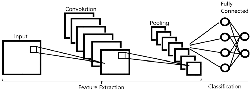
Classification process of a generic convolutional neural network.
Of existing research on the topic of winter RSC classification, that by Fu et al. ( 4 ) is one of few that analyzed the potential of using CNN in classifying RSC. In their study, images were collected from patrol vehicles that travel along a provincial highway. These images were then manually categorized according to three different classification systems, five-class, three-class, and two-class RSC systems, all of which were related to the extent of snow coverage. Using the classified images, five different machine learning models were developed and compared—ANN, CNN trained from scratch, pre-trained CNN, random forest, and random tree. In all three RSC classification systems, the pre-trained CNN model demonstrated the highest performance. Another topic addressed in this study is the effect of data size on CNN model performance. It was shown that increasing the number of images from 354 to 3542 increased model accuracy by 10%. The author concluded that model performance improves as data size increases.
In another similar study, Pan et al. ( 5 ) evaluated the performance of pre-trained residual-CNN in winter RSC classification. The pre-trained residual-CNN used in this study was developed from the ImageNet dataset, an image repository that contains over a million images; these are very generic images of animals, cars, clothing, and so forth. To tailor the model for RSC classification, additional tuning was performed on the residual-CNN model using rural road images taken from RWIS stations. Before fine-tuning could take place, these images were first categorized into one of four categories—bare, partly snow covered, fully snow covered, and not recognizable. For comparison purposes, three other ImageNet pre-trained CNN models were developed using the same RWIS image dataset—InceptionV3, Xception, and VGG16. All four pre-trained CNN models demonstrated high performance with classification accuracy over 90%, the highest being residual-CNN with an accuracy of 95.15%. Several other items were also examined in this study, one of which was the effect of data size on model performance. It was concluded that model performance can be further improved with an increased number of images. Another area explored was the concept of building on top of an existing RSC classification model. In situations where new data is acquired, instead of retraining the model from the beginning using new and old data combined, the developed RSC is trained additionally with the new dataset acquired. This updating process was shown to be capable of producing accuracy improvements with less training effort. In another paper, Pan et al. ( 6 ) would expand on this topic by adding two additional image sources—in-vehicle images and fixed traffic camera images. The same four pre-trained models were fine-tuned and compared, where although the best-performing model varied, the best-performing pre-trained CNN models all had accuracy over 90%.
Of the studies discussed thus far, the images used for model development have all been conventional images. Straying away from this trend, Nateghinia et al. ( 7 ) adopted use of infrared (IR) images as part of their model development process. To collect image data, an IR and a conventional camera were both mounted to the front of the vehicle. The vehicle was driven around the City of Montreal for data collection. For the RSC classification system, they used four classes: snowy, icy, wet, and slushy. This is quite different from the other two studies, as it focuses more on identifying the condition of the contaminant itself rather than the extent of contaminant coverage. For the CNN model, the researcher in this study proposed three CNN models: (1) CNN trained using only conventional images; (2) CNN trained using only IR images; and (3) a CNN model with two streams of input, one for IR images and the other for conventional images. Out of the three models, the two-stream CNN model displayed the best performance with classification accuracy of over 90%.
Instead of focusing solely on winter RSC, Cheng et al. ( 8 ) examined the performance of CNN on surface conditions year-round, which included dry, wet, snowy, muddy, and others. Although the study was focused more on determining the optimal activation function for CNN, it did offer an accuracy comparison between traditional machine learning techniques (SVM and ANN) and various forms of CNN models. The data used in this paper was not collected by the author but taken from several publicly available road image data sources with both rural and urban in-vehicle images. In model performance, traditional machine learning techniques were outperformed by CNN. CNN offered the highest accuracy of 94.89%, whereas SVP and ANN hovered around 85%. An additional evaluation was also performed on a general dataset containing images of aircraft, automobiles, birds, horses, and boats. In this labeling task, SVM and ANN were outperformed by a large margin. Both SVM and ANN did not exceed 60% accuracy, while CNN reached 93.93%.
Nolte et al. ( 9 ) also conducted a study investigating CNN performance on classifying general road conditions. This study has six categories: asphalt, dirt, grass, wet asphalt, cobblestone, and snow. Using a similar dataset to that used by Cheng et al. ( 8 ), two different architectures of CNN were evaluated, InceptionV3 and ResNet50. The author found both models to have accuracy around 90%, with ResNet50 slightly better by about 2%.
There is one other notable study by Carrillo et al. ( 10 ). In this paper, the researchers developed their own CNN model for RSC classification and compared its performance to six different ImageNet pre-trained CNN models. These models were all developed using images from RWIS stations, categorized into bare, partially snow covered, and fully snow covered. Post model development, the results showed that the researchers’ model had a classification accuracy of 93%, outperforming all pre-trained CNN models in accuracy and training speed.
Overall, as seen from the literature discussed in this section, previous studies on the topic of winter RSC are centered around developing RSC classification models for rural highways; only one study— Nateghinia et al. ( 7 )—developed an urban model, but it was designed for contaminant identification, not for RSC classification. Furthermore, in respect of model development itself, previous studies either developed their own original CNN model from scratch or focused on repurposing a pre-trained ImageNet model. Based on these research trends observed, two limitations are identified: the lack of studies that focus on developing a highly transferable urban RSC model; and limited exploration of repurposing a pre-trained RSC model, both of which serve as motivations for our proposed study.
Methodology
Data Collection, Processing, and Integration
The image dataset used in this study was collected from Canada’s fifth most populated city, Edmonton ( 11 ). The study area is located on the south side of Edmonton and contains three regions: the Heritage Valley Neighborhood, Highway 2, and Highway 216. These regions were chosen in an effort to encompass all road types found in an urban environment. Heritage Valley contains arterials, collectors, and neighborhood local roads, whereas Highways 2 and 216 are representations of intracity highways found in Edmonton. The areas selected for this study are highlighted in red in Figure 2.
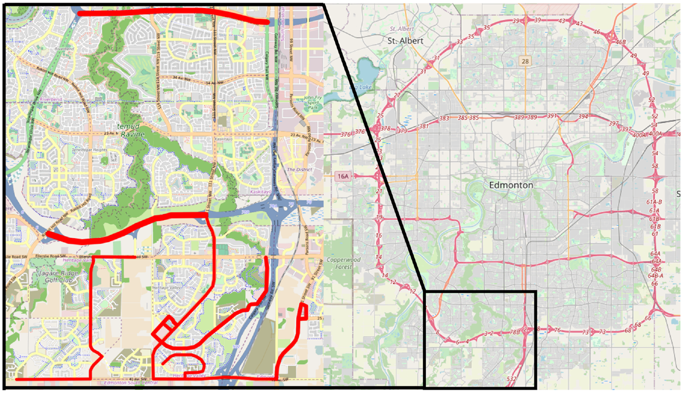
Study area: Edmonton, Alberta.
To capture winter RSC images, a vehicle equipped with a GoPro HERO9 camera was driven around the study area for a total of 47 km near the end of February 2021. During the data collection process, footage of all desired road types with varying levels of snow coverage was recorded. Once enough data was collected, the recorded footage was converted into images at a rate of one image per second of video. This rate ensures that a sufficient degree of variation exists between images without drastically cutting down data size. Using a similar RSC categorization system to one used by previous studies ( 5 ), all images were categorized into one of four categories: bare, partially snow covered, fully snow covered, and undefined. A breakdown of the classification system used is depicted in Table 1. To maintain consistency in the labeling process, the labeling of RSC was completed by one person in accordance with the RSC description column in Table 1, which eliminates the issue of varying interpretations of what each RSC category is when multiple labelers are involved. On completing the labeling process, the labeled images were then organized into four folders based on their respective RSC label. At that point, a second check was done to correct any mislabels.
Road Surface Condition (RSC) Categories
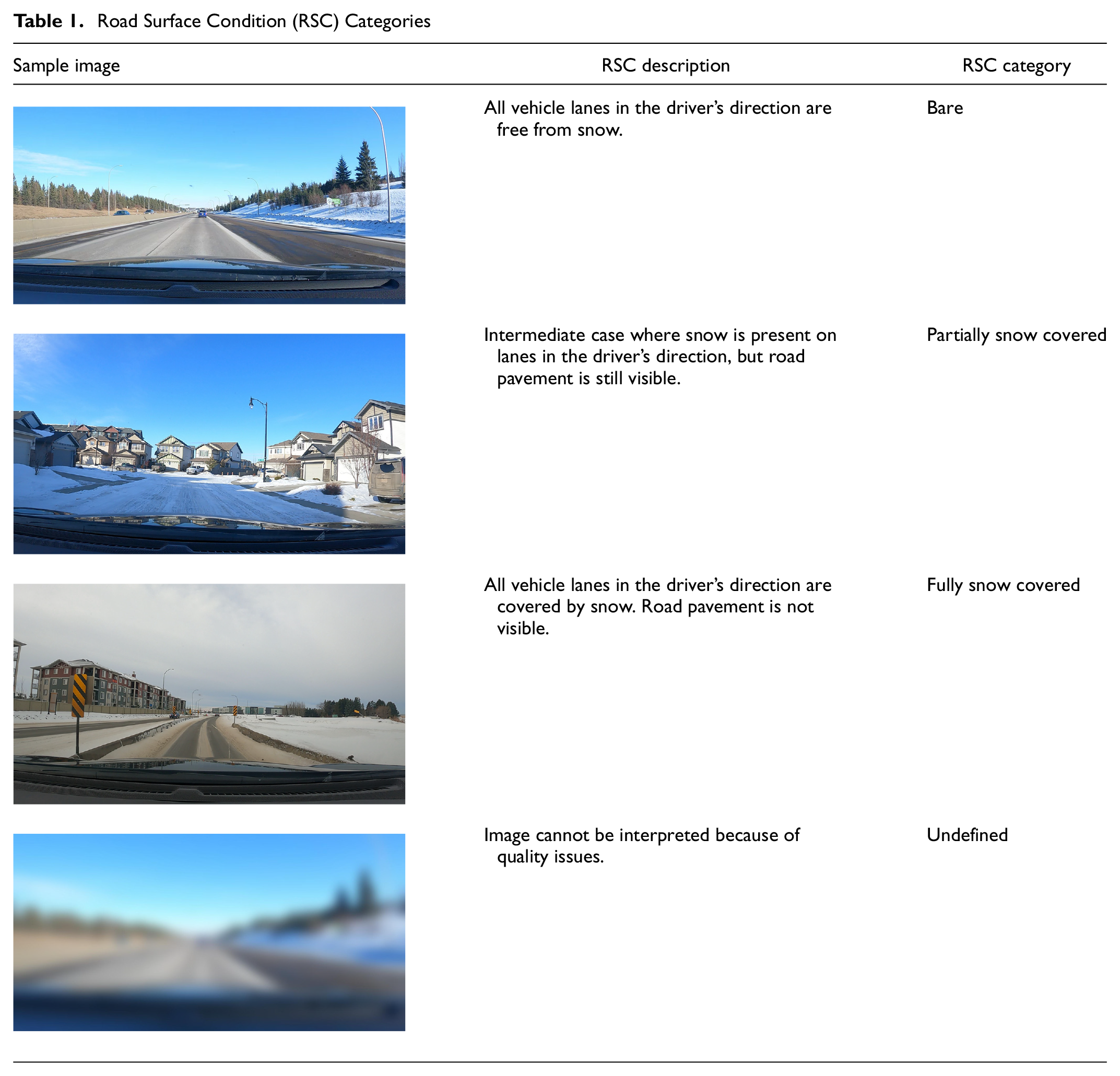
Because of the quality of the camera used and driving conditions during the time of recording, quality of the footage collected was extremely high, so much so that no images were found to be unrecognizable. Nevertheless, this is unrealistic as sun glare, rain, snow, and so forth, are all likely to distort the image at some point. To account for this in our image dataset, equal numbers of images randomly chosen from each of the three classes were blurred to represent the undefined class.
In total, 3914 images were manually classified. Among them, 1001 images were bare lane, 1541 were partially snow covered, 685 were fully snow covered, and 687 were undefined. Figure 3 depicts the image distribution of the collected dataset.
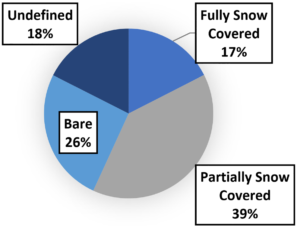
Distribution of images collected.
Urban Winter Road Conditions Classification Model
The overall model developmental framework used in this section is illustrated in Figure 4. Collected data will first be inputted into two models that share identical CNN architecture but differ in training method. One model will be trained using transfer learning with a pre-trained RSC model, whereas the other will be trained from scratch. And as part of additional fine-tuning, training depth evaluation (number of layers fine-tuned) and different 1-D feature conversion strategies will be investigated for how they influence model performance. The most accurate model developed via transfer learning will then be compared with the model trained from scratch. This comparison will include an accuracy evaluation as well as a data sensitivity analysis to determine whether there are benefits associated with transfer learning. Between the two training methods, the best-performing model will then undergo hyperparameter optimization to enhance model performance further, outputting our final urban RSC model.
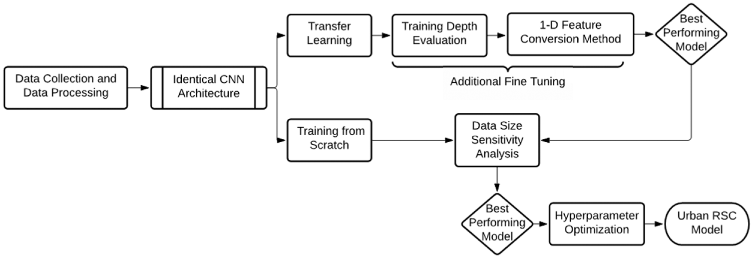
Road surface condition (RSC) model development framework.
The CNN architecture used for both training methods was originally developed by Carrillo et al. ( 10 ). While the feature extraction layers were kept the same, the FC layers were changed to two dense layers with 1000 neurons. This change was made as suggested in literature, where the best-performing FC layer architecture was shown to be two dense layers with 1000 neurons each ( 6 ). An overview of the entire CNN architecture is shown in Figure 5.
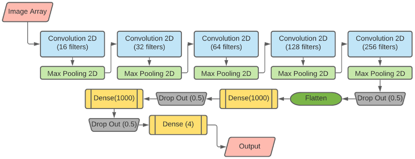
Convolutional neural network architecture used in this study.
To give a brief overview of the architecture, the image array gets passed through five cycles of convolutional-pooling layers to reduce array size, and at the same time, extract an increasing number of feature maps by doubling the number of filters each cycle. Post feature extraction, the extracted feature maps are flattened into a 1-D array and are passed into the FC layer with two 1000-neuron dense layers. The output of the FC layer then gets passed into the classifier—the 4-neuron dense layer—where it is converted into a probability vector output.
Before training the model, the image dataset was split 80/20, with 80% of data allocated to training and 20% allocated to validation. In addition, the image array was normalized to be within [0,1], and its matrix dimension was reshaped to [224,224] to align with the input requirements of the pre-trained model. All model training were performed using KERAS with an NVIDIA T4 or P100 GPU and 13 GB of RAM available on the GOOGLE Colaboratory platform (20). During the training process, any CNN model adjustments were made purely based on the training dataset. The validation dataset (i.e., unseen images) is only used at the end of an epoch—one complete pass through the entire dataset—to give the researcher unbiased model performance feedback.
When evaluating the performance of CNN network, two variables were tracked in this study: accuracy and loss. Accuracy is based on whether model classification is equivalent to the actual class. Loss, on the other hand, is determined using cross-entropy loss, which is the difference between the true distribution and the predicted distribution. Equation 1 gives the formula for cross-entropy loss where the true distribution is a one-hot vector—a vector containing all 0s except for one entry set to 1.

where
The reason accuracy and loss are tracked during training is to look out for overfitting. Overfitting is when the CNN model is fitted too closely to the training dataset, rendering it unable to generalize new data. This is commonly observed when the training dataset displays high accuracy and low loss, but when validated, accuracy is low and loss is high ( 12 ).
Transfer Learning
CNN model architecture is complex and challenging to develop. In the field of CNN, there are currently no set rules when it comes to model design. Architecture design is nearly entirely based on subject area expertise and trial and error. Furthermore, CNN model development is also heavily dependent on computer hardware. The greater the number of convolutional and pooling layers, the more resource-heavy it is to train. This creates a situation where deep CNN models can only be trained by state-of-the-art computers. To get around these barriers, we proposed developing our model based on a process called transfer learning. Transfer learning is the process of taking an existing pre-trained model and repurposing it. This process is based on the idea that features captured in the initial layers are generic features, and features captured deeper in the CNN are more dataset-specific ( 13 ).
The process of transfer learning can be broken down into two steps: 1) freeze feature extraction layers and 2) train CNN with new image dataset. Freezing layers maintains the feature extraction process; the new image dataset will not modify these layers, thus decreasing computer resource demand. The most common practice is to freeze all feature extraction layers and train only the FC layer. This is because the FC layer is the most dataset-specific portion of the CNN. Therefore, the layers must be modified when classification categories are changed. Once the FC layer has been tailored to the new dataset, the feature extraction layers near the FC layer can be unfrozen and fine-tuned using the new dataset to tailor the model further.
There are several benefits of using transfer learning—one being the ability to develop models with a substantially smaller dataset than is usually required; another being enhanced training speed as we are only training the dataset-specific portion of the network, which is typically a small portion of the CNN architecture. However, to take advantage of these benefits, data used for transfer learning must be preprocessed in the same manner as the pre-trained model; otherwise, we will not be able to take advantage of the generic feature extraction layers.
Hyperparameter Tuning
The performance of CNN models is not solely dependent on the order and number of layers; there are many other factors such as the number of neurons in the FC layer, model learning rate, and regularization dropout probability. Together, these factors are called hyperparameters and are tuned in the model development process to increase model performance. There are, however, several problems with hyperparameter tuning. One is that the hyperparameter search space is vast, and it is unclear which hyperparameter should be tuned; this makes the searching process extremely lengthy. Another issue is that different image datasets may require different hyperparameter configurations; therefore, hyperparameter optimization may need to be redone whenever the dataset changes. To optimize hyperparameters efficiently, multiple optimization strategies have been developed. Among them, hyperband and Bayesian optimization are two that have demonstrated good performance and are therefore acknowledged in this study.
The hyperband optimization method uses the successive halving technique, where a set number of hyperparameter configurations are initialized and evaluated with an initial resource budget. Half of the worst-performing configurations are eliminated, and the remaining models are evaluated again but with double the budget ( 14 ). This cycle continues until one hyperparameter configuration remains. Figure 6a is a depiction of the successive halving technique.
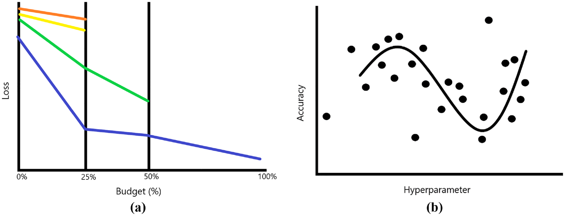
Hyperparameter optimization methods used in this study: (a) successive halving and (b) Bayesian optimization.
Bayesian optimization functions by mapping hyperparameter values against a performance objective, which creates a surrogate function to determine the most promising hyperparameter configuration. With each new iteration, the surrogate function evaluates what it believes to be the best combination and updates itself based on the performance recorded. With enough iterations, the surrogate model should be able to reveal the true relationship between the hyperparameters and the performance objective. Figure 6b shows an example of a simple Bayesian optimization. The black dots are recorded observations, and the black line represents the constructed surrogate function ( 15 ).
Results and Discussions
In our recent efforts with the same architecture shown in Figure 5, we developed an RSC CNN model using over 10,000 in-vehicle images collected from rural highways ( 16 ). The developed model displayed high performance of over 90% accuracy in labeling all four RSC categories, combining to a total of 94.6% accuracy overall. Because of the dataset similarity and high-performance results, our developed RSC model will be used as the pre-trained model in this study. But before transfer learning is applied to repurpose the pre-trained model, it is important to evaluate the model without any fine-tuning to establish a baseline performance measurement.
Using the validation images (i.e., urban road images) collected in this study as input, the pre-trained RSC model was tasked with classifying the RSC of each image. The performance accuracy for each RSC category is shown in the confusion matrix given in Table 2.
Performance Results from Road Surface Condition Classifications Made by Pre-Trained Model
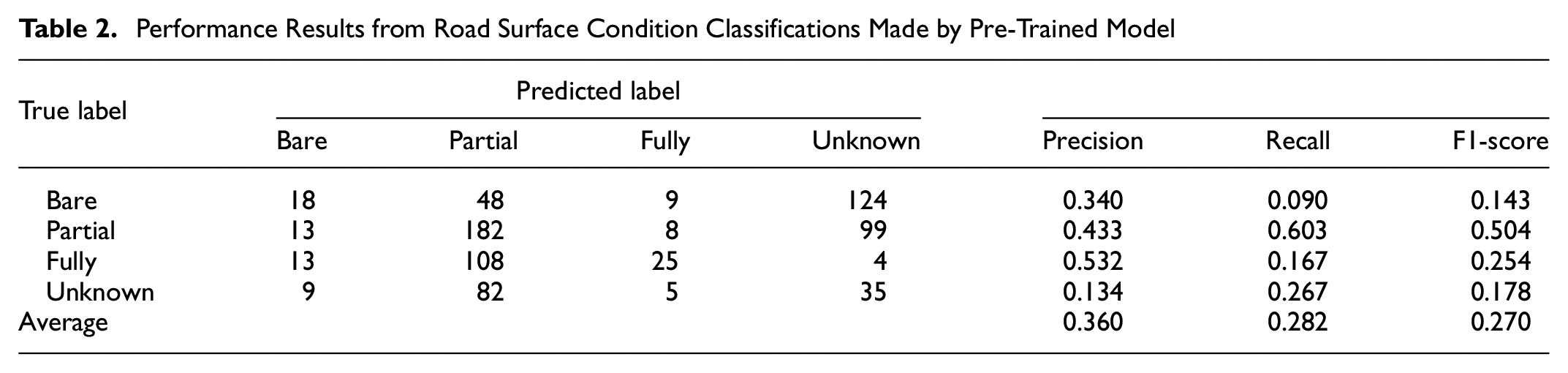
The pre-trained model had an accuracy rate of 33%, far lower than the 94.6% reported when using a rural highway image dataset ( 16 ). Table 2 further breaks down the model performance by showing each RSC class’s precision, recall, and F1-score. For all three performance measures, the vast majority are below 50%, meaning the model produces a significant amount of false labels. The only exceptions are precision for fully snow covered, and recall and F1-score for partially snow covered, which is a sign that the pre-trained model contains transferable feature extraction layers that we can use to our advantage.
Overall, the pre-trained RSC model performed poorly with the urban dataset, which is likely because of changes in road surroundings. In the rural RSC dataset, there are often few cars visible in the surrounding area and no pedestrians or buildings. The sudden introduction of these new environmental variables is likely to have confused the model, resulting in a drastic drop in performance.
Transfer Learning with Pre-Trained Model
As discussed in the previous section, the introduction of new variables in the urban image dataset severely diminished the performance of our pre-trained RSC model from 94.6% to 33%. To counteract this change, transfer learning was applied to fine-tune the pre-trained model to the urban environment using the 3914 images collected in this study. But before introducing the urban RSC dataset to the model, all layers with the exception of the FC layer were frozen, making it only possible to train FC’s dense layers.
In this study, model accuracy and loss were recorded every epoch (one pass through the entire dataset) to track training progress. And in effort to avoid overfitting, a stopping criterion was implemented into the training process. If the loss did not decrease within 12 epochs, the model was assumed to have plateaued, training was stopped, and the model was restored to the state with the lowest loss; the red dot in Figure 7 represents the model plateau point.
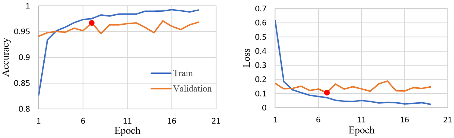
Accuracy and loss per epoch recorded during transfer learning.
As shown in Figure 7, after only one epoch, the pre-trained model’s validation accuracy soared to 94.12%. With additional training, the model’s performance gradually improved until the validation accuracy peaked at 96.68%. In respect of loss, a similar pattern was observed. With only one epoch of training, the validation loss dropped to 0.172 and gradually decreased until the minimum was reached at 0.106. In general, the model reached peak performance extremely quickly as only seven epochs were needed. This behavior may be caused by existing RSC feature extraction filters, as the pre-trained model was not learning how to extract RSC features but simply calibrating itself to the new urban environment. Compared with similar studies, where the training process is observed to take much longer—30+ epochs (6, 8)— calibration may be much faster than learning from square one. Another observation is that validation and training accuracy had similar trends in accuracy and loss throughout training, with minor differences between the two lines, indicating that the modifications made based on the training data can be generalized to the validation dataset. Thus, overfitting was not a significant concern during the training process.
Additional Fine-Tuning
Once the FC layer has been tuned, the model can be further fine-tuned by unfreezing the feature extraction layers closest to the FC layer. By unfreezing additional layers, the aim was to determine whether fine-tuning more of the network is beneficial to model performance; and if so, at which layer. There was a total of five convolutional-pooling layer groups; these layer groups were unfrozen incrementally starting from the layer closest to the FC layer. But before increasing the number of unfrozen layers, the CNN model was restored to a state where only the FC layer had been trained. This was done to avoid the magnitude of the model changes from being too large, destroying everything the pre-trained model had previously learned ( 13 ). The result from this analysis is illustrated in Figure 8.
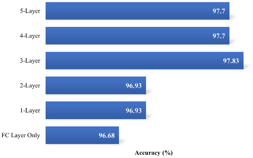
Convolutional neural network transfer learning depth analysis.
Looking at Figure 8, it can be observed that the model accuracy improved as the number of layers increased from one to three, reaching peak accuracy of 97.83% at three layers. Soon after, the model performance dropped slightly at four and five layers to 97.7%. This overall trend was expected. As mentioned in the methodology section, features most specific to the dataset are located in the FC layer. The closer the layer is to the beginning of the network, the more generic the feature extraction process. When layers closest to the FC (one to three layers) were fine-tuned, the performance was observed to increase from 96.68% to 97.83% because the feature extraction process more specific to the dataset got calibrated to the urban environment; and as layers farther away from the FC (four to five layers) got adjusted, a minor decrease from 97.83% to 97.7% was recorded; this is because feature maps considered generic to RSC classification got fine-tuned when they do not need to be, thus resulting in a minor performance drop. However, fine-tuning four and five layers of the CNN still outperformed fine-tuning one to two layers FC only, suggesting that tuning more than 50% of the feature extraction layers may yield performance improvements when developing an urban model using transfer learning. It is also important to note that increasing depth of training may decrease training speed, as you are retraining a greater portion of the network.
Recall that the CNN model architecture shown in Figure 5 uses a flatten layer between the feature extraction and FC layer interface, which takes any feature map and converts it into a 1-D array without any additional processing to reduce the size of the 1-D array sent into the FC layer. Other than flatten, two other 1-D conversion operations exist—global max pooling and global average pooling, which take either the maximum or the average of each feature map matrix; therefore, they can heavily reduce the size of the 1-D array sent into the FC layer, thus increasing training speed. Additionally, in past literature, global average pooling has been suggested to provide better correspondence between feature map categories ( 17 ), which may increase a model’s performance. To evaluate the performance of these alternative methods, the same procedure used in training depth evaluation was used to evaluate each of the strategies at different depths of training. The results are shown in Figure 9.
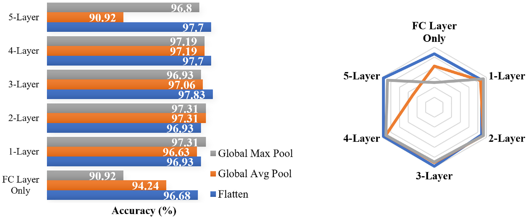
Comparison between strategies to convert feature maps into 1-D array.
Based on Figure 9 it would appear that flatten offers the best performance out of the three 1-D array conversion strategies. Other than fine-tuning at one and two layers above the FC layer, flatten outperformed the two other methods. In performance change with respect to the number of layers tuned, all three methods displayed a similar pattern. All exhibited performance improvements from FC only to two or three layers, at which point the performance peaked and began to drop. Overall, it would appear that regardless of the 1-D array conversion strategy, for this specific CNN architecture, fine-tuning two to three layers of the feature extraction layer alongside the FC layer yielded the best result. This is likely for the same reason as mentioned earlier, that performance improves when data-specific layers located near the FC layer are calibrated, but when generic feature extraction processes located at the beginning of the network get tuned, model performance drops.
Training Method Comparison
To compare performance between the transfer-learning model and models trained from scratch, a CNN model was developed from scratch using the same urban RSC dataset and identical architecture. The training process was recorded and illustrated in Figure 10.
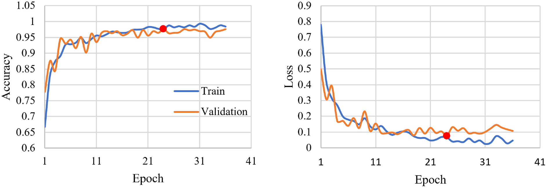
Accuracy and loss per epoch for model trained from scratch.
On closer inspection of Figure 10, it was observed that the changes in accuracy and loss were much more gradual than with transfer learning. After one epoch, validation accuracy increased to 77% as opposed to the 94% observed in transfer learning. This is likely because of the existing feature extraction process present in the pre-trained model, as it has already learned to recognize RSC in the past. After one epoch, the pre-trained model quickly adjusted to the new dataset, whereas the model trained from scratch was still learning and undergoing major changes. As the model got exposed to greater epochs, its performance gradually increased until epoch 24, where peak accuracy of 97.57% was reached. Compared with transfer learning, although it had higher accuracy than a pre-trained RSC model with only the FC layer tuned, it reached peak performance 17 epochs slower, and it also did not outperform the 97.83% achieved when three layers were fine-tuned alongside the FC layer.
Data Size Sensitivity Analysis
Other than comparing accuracy between transfer learning and training from scratch, it is also important to examine the data size requirements for each model. For this purpose, a sensitivity analysis was performed to examine how data size affects model performance. To perform this analysis, images were added in increments of 100 up to a total of 3914 images. Any additional images were added on top of the existing ones, that is, 200 images contained all images found in 100 images. Additionally, the pre-trained flatten model with three layers fine-tuned was used to represent transfer learning. Figure 11 shows the validation accuracy recorded from this analysis.
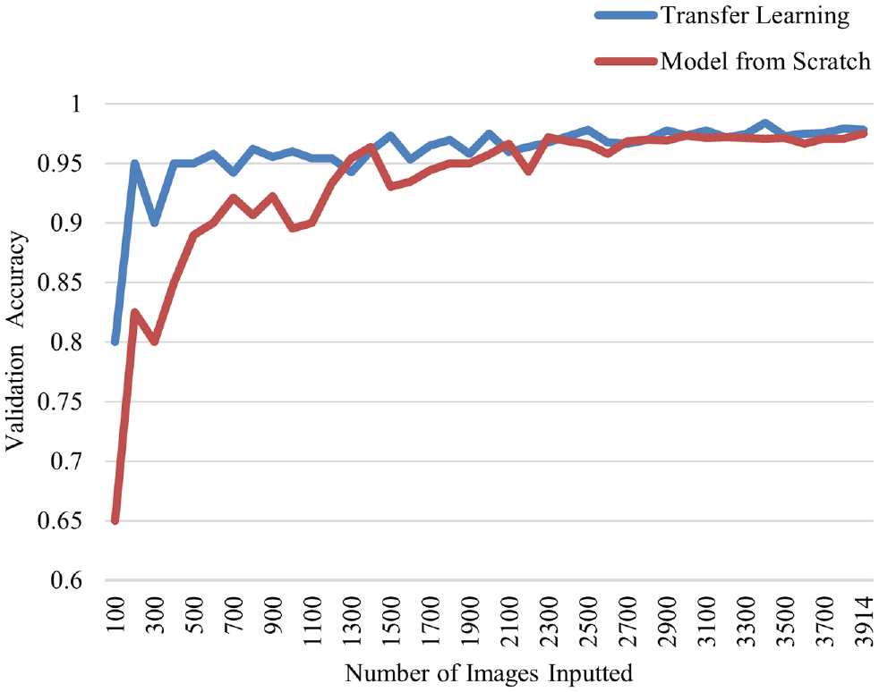
Data size sensitivity analysis.
By looking at Figure 11, it is evident that model performance increased as the size of the dataset increased for both methods. Nevertheless, transfer learning seemed to have improved at a much faster rate than its competition. At 100 images, a large accuracy gap was present; transfer learning reached 80% accuracy, whereas training from scratch only reached 65%. This large gap would extend to 200 images where the transfer-learning model improved to 95% accuracy, while its competition reached 82.5%. It was not until 1300 images where the gap closed. From 1300 images onward, both models showed an approximate 2% total increase in accuracy over the course of 2600 additional images. Between the two training methods, transfer learning showed less overall sensitivity to data size. It was able to reach high accuracy very quickly with minimal data size requirements. Since the RSC pre-trained model could already make generalizations about RSC, it only required a few images to calibrate itself to the new urban RSC dataset. On the other hand, the model trained from scratch did not have any preexisting knowledge on RSC classification. It was essentially learning from scratch about how to classify RSC; therefore, it started at a low accuracy rate of 65% and improved much more overall, 32.5% versus 18% observed from transfer learning.
Hyperparameter Optimization
Based on the analysis completed thus far, transfer learning with pre-trained RSC model seems to be the best performing. In this section, we present a method called hyperparameter optimization to improve model performance further. Thus, a hyperparameter search was set up using hyperband and Bayesian algorithms as discussed previously. Because the hyperparameter search domain is very large, in this study, four hyperparameters in the FC layer were targeted: dropout rate, a technique to disable a portion of the neurons during training to prevent overfitting ( 18 ); the number of neurons in dense layer 1 of the FC layer; the number of neurons in dense layer 2 of the FC layer; and learning rate (controls how quickly the model learns from the inputted dataset). Once the optimal hyperparameter configuration was discovered, transfer learning would be applied to evaluate the model’s performance. Figure 12 below depicts the hyperparameter optimized FC layer architecture. Values modified are highlighted in red.
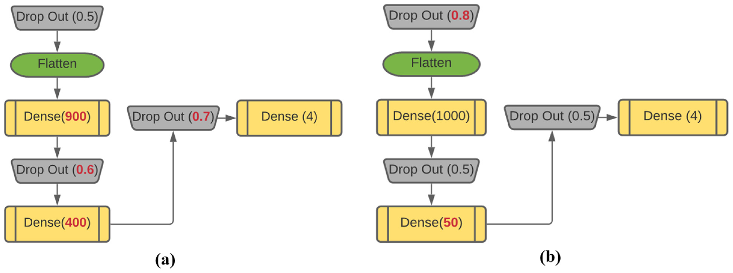
Hyperparameter optimized fully connected (FC) layer architecture: (a) hyperband and (b) Bayesian.
Using the Bayesian optimizer, a performance increase from 96.68% to 96.8% was observed when only FC was trained; and when fine-tuned further, tuning all five layers yielded the highest validation accuracy of 97.7%. In comparison, hyperband was able to improve validation accuracy from 96.8% to 97.7%, and with additional fine-tuning, 98.2% was recorded when four layers were tuned, which exceeded the best-performing model so far, making it the best-performing urban model in this study. Figure 13 depicts the performance of the hyperparameter optimized models and how they compare with the best-performing model discovered in this study thus far.
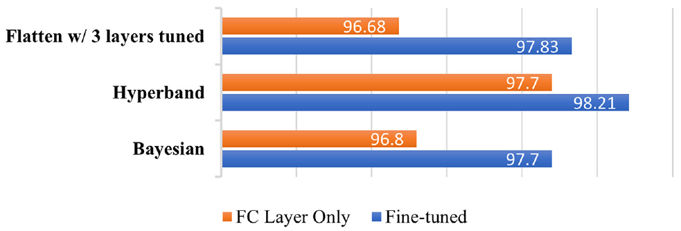
Performance comparison between models developed in this study.
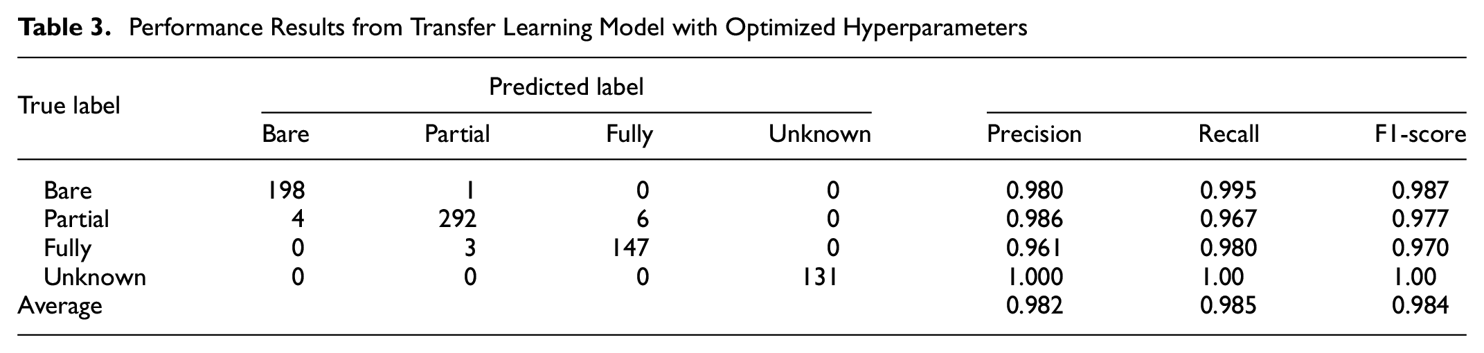
Additionally, using the best-performing model developed in this study—the hyperband optimized model—the performance of the hyperparameter optimized model was evaluated to illustrate the improvements made per category using a combination of transfer learning and hyperparameter optimization. This evaluation was made with the validation dataset, containing 199 images of bare lane, 302 partially snow covered, 150 fully snow covered, and 131 undefined. And as depicted in Table 3, model performance increased substantially across the board. Precision increased from the sub-50% rates shown in Table 2 to over 96% for all categories. Comparatively, the number of false positives (FP) was minuscule in each category. Other than the fully snow-covered class that had a 4% FP rate, every other class was below 2%, which is far lower than the 60%–90% observed in the pre-trained model before transfer learning. Likewise, recall and F1-score saw similar improvements. Before transfer learning, the pre-trained model predicted far too many false negatives (FN) for bare, partial, and unknown categories, which is reflected by their poor recall percentage of 9.0%, 16.7%, and 26.7%, respectively. Post transfer learning, recall for all categories increased to above 95%. And since the F1-score is a harmonic mean of precision and recall, the improvements made to these two measures improved the F1-score from 27.0% to 98.4% overall. Therefore, our developed urban RSC model is particularly robust, as it can correctly classify all four categories with very few FPs and FNs.
Performance Results from Transfer Learning Model with Optimized Hyperparameters
Conclusions
The use of CNN to automate the process of RSC classification can be an extremely effective technique to provide real-time RSC information, allowing maintenance personnel to combat inclement weather in a timely and efficient manner. Recorded images can be uploaded into the CNN model as they are collected, providing minimal delay between image collection and image classification. To date, researchers have been focused on designing models for rural highways with very little attention placed on municipal road networks. Furthermore, model development itself tends to focus on creating custom models trained from scratch or by using transfer learning with ImageNet models. Very few studies have looked at using transfer learning with a pre-trained RSC model. To address these gaps, we collected over 3000 images within a neighborhood south of Edmonton, Alberta, covering most municipal road types—freeways, arterials, collectors, and neighborhood roads. Using these images, we developed a robust urban RSC classification model by applying transfer-learning techniques to an existing pre-trained RSC model that was developed using rural highway images. Several techniques were used throughout this study to boost model performance: fine-tuning transfer-learning depth, changing feature map to 1-D array conversion method, and hyperparameter optimization.
To summarize the results recorded, at the very start of development, the performance of a pre-trained RSC model without any modifications was evaluated to test transferability, which yielded only a 34% accuracy rate. Next, to boost the model’s performance, transfer learning was used to tune only the FC layer of the rural pre-trained model to calibrate its feature extraction processes to the urban environment, resulting in a performance boost to 96.68% validation accuracy. And in effort to increase model performance further, training was extended into the feature extraction layer to fine-tune the feature extraction processes, which increased model accuracy to 97.83%. We also evaluated alternative ways to covert feature maps into 1-D arrays, which revealed that among flatten, global average pooling, and max pooling, flatten displayed the best performance.
With an urban RSC model developed using transfer learning, a CNN model trained from scratch was also developed using identical architecture and image dataset for comparison purposes. Although the model trained from scratch exhibited high accuracy of 97.57%, it was still outperformed by transfer learning with three layers fine-tuned. And when training efficiency is considered, training from scratch required 17 more epochs for the model to reach peak performance, making it less efficient and less accurate when compared with transfer learning. Furthermore, the two different training methods’ sensitivity to data size was also examined, revealing that the model developed from transfer learning required less data to reach high accuracy, and therefore, was less sensitive to data size. Finally, a hyperparameter optimization was performed on the best-performing model found in this study, elevating the transfer-learning model accuracy one last time to 98.21%. Throughout the development process, there are cases where the model accuracy improved by less than 1%, which raises the question whether such marginal improvements involving much added effort would result in any noticeable difference from the user perspective.
In respect of future research, the comparison between transfer-learning models and models developed from scratch can be improved using a larger dataset. It was observed in the sensitivity analysis that the performance accuracy for both training methods slowly converged as dataset size increased. But because of the lack of data, it is unknown whether training a model from scratch would outperform transfer learning at some point; only when more data is available can this question be answered. In addition, the categories themselves can be expanded on to represent a more diverse set of conditions. For example, the partially snow-covered class can be broken down into more specific categories like two-track bare and one-track bare lane, and new descriptors like icy and wet can be added to describe each RSC further. Another area of future research is using a more complex CNN architecture. The architecture used in this study is rather simple compared with the more recent CNNs developed, such as EfficientNet ( 19 ). There is merit in using a more recent architecture to test if more complex architectures yield higher performance results. Furthermore, when connected vehicle systems become more widely available, the data their sensors and cameras detect can be used as an important data source for model development. What additional road surface variables can be determined using connected vehicle data is another topic worth exploring. Finally, it may be possible to design a framework that automatically provides real-time RSC information based on dash camera images. The output of the RSC model can be combined with the location of where the image was taken to provide a spatially continuous view of RSC for any road network.
Footnotes
Author Contributions
The authors confirm contribution to the paper as follows: study conception and design: Qian Xie, Tae J. Kwon; data collection: Qian Xie, Tae J. Kwon; analysis and interpretation of results: Qian Xie, Tae J. Kwon; draft manuscript preparation: Qian Xie, Tae J. Kwon. All authors reviewed the results and approved the final version of the manuscript.
Declaration of Conflicting Interests
The author(s) declared no potential conflicts of interest with respect to the research, authorship, and/or publication of this article.
Funding
The author(s) disclosed receipt of the following financial support for the research, authorship, and/or publication of this article: The authors would like to acknowledge the Alberta Ministry of Economic Development, Trade, and Tourism (Minister) for providing financial support. This study was also partially funded by National Sciences and Engineering Research Council of Canada (NSERC).