Sage Journals: Discover world-class research

Abstract

Planners have theorized that transitioning commuter rail systems to regional rail networks will increase ridership, balance mode share, and reduce automobile use in North American cities. This process is currently underway in Ontario, Canada, as service is being expanded throughout the GO Transit commuter rail network. Calculating elasticities is a common approach used to identify factors that, if adapted, may significantly influence transit demand. However, few studies have focused on identifying demand elasticities specific to the current case of upgrading commuter rail systems in the North American context. The purpose of this study is to fill this gap. Station-level ridership data were compiled for the GO system from January 2016 to December 2019. Smartcard data were used to estimate station catchment areas for which land use, socioeconomic, and demographic datasets were developed. Data about additional factors related to station access, service quantity, fare price, and availability of substitute transport modes were also compiled. Controlling for trip type (e.g., a.m. peak and evening off-peak), demand models were estimated using a random effect panel data estimator. This study finds that service quantity, population density, fuel price, and unemployment rate were significantly associated with commuter rail ridership, regardless of trip type examined. Employment density and seasonal variation were also significant, although different signs were shown between models. The results suggest that plans for this kind of transition should include other considerations in addition to service quantity improvements. Those directed toward the implementation of transit-oriented developments, transport pricing schemes, and competitive fare price strategies are outlined.

Keywords

planning and analysis pricing elasticity of demand public transportation rail transit systems commuter rail heavy rail urban rail ridership

In the post-World War II era, North American transportation investments have focused disproportionately on accommodating automobile users, as the construction of roads and expressways has often been prioritized over transit service expansions ( 1 ). Subsequently, over 80% of travel in some North American regions is completed via private automobile. As metropolitan areas expand, planners are struggling to react to increased levels of congestion, greenhouse gas emissions, and other negative externalities realized as a result of an uneven mode share.

European examples have shown that rail networks can effectively serve inter-regional trips. These systems facilitate the movement of people from city suburbs into neighboring metropolitan areas, while operating with 5–20 min headways on all lines throughout the day ( 2 ). They also have numerous advantages when compared with private automobile in relation to speed, capacity, urban space consumption, and reliability during peak commuting periods. Various studies have suggested that, when these conditions are accomplished, ridership is stimulated, thus resulting in a mode share that is more evenly distributed ( 3 ).

Recognizing this, many North American regions are planning to upgrade existing commuter rail systems—those operating in peak periods with an emphasis on journey to work trips—to regional rail networks, with more complete operating hours, serving more diverse origins and destinations. Level of service improvements are often the focus of these plans, as planners have theorized that mode share will move toward greater balance if quick, competitive, and convenient alternatives are provided. However, service quantity is just one factor that stimulates demand for transit, as ridership may be equally responsive to other influences both internal and external to the transit agency ( 4 – 6 ). Additional interventions might be needed to effectively stimulate demand and encourage mode shift in these areas.

Econometric analysis is often conducted to explore relationships between ridership (demand) and various factors, supporting the development of policy directions that transit planners should consider. However, few studies have solely focused on assessing the sensitivity of commuter rail ridership in relation to potential operating and demographic factors that can influence demand. Using southern Ontario’s GO Transit commuter rail system in Canada as a case study, this paper presents demand elasticity models to further explore these relationships.

The first section of this paper reviews prior evidence on the relationships between station-level ridership and factors that influence mode choice decisions. The second section describes the study area and various research methods used. The third section presents demand elasticity estimates, obtained from the application of random effect linear panel data models, seperated by trip type. The paper concludes with discussion surrounding the theoretical and practical application of this work.

Literature Review

The current study attempts to estimate potential changes in demand for an existing commuter rail system that may emerge as a result of its upgrading to a regional rail system. While this focus is novel, the general area—understanding the likelihood of change in demand resulting from modifications to system design and operation—has been actively researched. This section presents relevant literature that informs the current work.

Demand Elasticity Methods

Regression analysis is commonly used to understand how the demand for a good or service is influenced by economic factors affecting the customer. Essentially, model outputs can be used to identify which independent variable(s) is/are most important in influencing the dependent variable, and estimate how the dependent variable should respond if change in the independent variable(s) occurs ( 7 ). Since slope estimates can be used to obtain demand elasticity values, researchers can estimate the relationship and impact of multiple variables on transit demand, including transit fares, travel times, service supply, service attributes, passenger characteristics, prices of alternative transport modes, urban characteristics, and regional characteristics ( 6 ).

Factors Associated with Demand

Demand was originally theorized to be predominantly responsive to fare price, as in the seminal work of Curtin, which estimated a fare price elasticity of −0.3 ( 8 ). Otherwise known as the Simpson-Curtin rule, this benchmark is still widely used by transit planners when evaluating the impact of fare price changes on ridership ( 9 ). Since then, additional characteristics, including those related to the system’s service area’s regional geography, metropolitan economy, socioeconomic, and automobile/highway system, have been found to influence ridership to varying degrees ( 4 – 6 ).

Mode-specific studies have found that commuter rail ridership is inversely affected by change in some factors compared with conventional transit demand. For example, a study of rail ridership in California found that fare price significantly influenced demand in only half of the systems included in their analysis, while a similar study in the State of Washington found a statistically insignificant elasticity of −0.04 ( 10 ). Durning and Townsend excluded fare price from their final models entirely because of insignificance ( 11 ). Recent studies have attempted to quantify the main determinants of commuter rail ridership, but excluded fare price as a candidate variable altogether ( 12 – 14 ). This could suggest that data availability in relation to this variable is hard to obtain, interpret, or both, because of the zonal or distance-based fare schemes commonly used by commuter rail agencies, and/or suggests that fare price does not influence commuter rail ridership to the same degree as conventional transit demand.

Further, demand elasticity estimates can differ depending on the geographical context of the study. Balcombe et al. found that demand is twice as sensitive to fuel price in North America compared with Europe, while an analysis of rail ridership in the Washington D.C. and Maryland area found that ridership was only responsive to the presence of feeder bus connections ( 4 , 13 ). An analysis of rail rapid transit ridership in Canada further found that demand was most responsive to the provision of feeder bus connections and park and ride infrastructure ( 11 ). This may be a result of increased automobile ownership rates in North American regions, resulting in more pronounced demand relationships between ridership and change in these factors.

Various studies have highlighted quantitative considerations that should be controlled for to increase the accuracy of models used to estimate demand changes. Studies that controlled for trip type (e.g., commuting or discretionary) have found that ridership during the a.m. peak period is significantly correlated with population density, while employment density had a greater impact on demand in the afternoon ( 12 , 15 ) Schimek further notes lags between service quantity changes and shifts in demand patterns, while studies that focused on quantifying the relationship between fuel price changes and ridership have established similar trends ( 9 , 10 , 16 , 17 ). Therefore, the literature indicates that demand elasticities could be understated if trip type is not controlled for, or if the time-series analyzed does not capture long-term effects.

Delineating Station Catchment Areas

Station catchment areas are often used to extract external variable datasets included in demand elasticity studies. Determined as a function of the distance a transit user is willing to travel to access a station, circular buffers (or sometimes more sophisticated spatial variants) ranging in distance from 400 to 800 meters are commonly implemented around a given station ( 18 ). External variable datasets within these buffers are then extracted for further analysis.

However, an analysis of station access behavior of GO Transit rail users in Ontario, Canada, suggested that the use of 400 to 800 meter arbitrary buffers is not applicable for commuter rail systems, as most passengers access the system via automobile ( 19 ). The authors instead used survey data to map customer origin locations. A convex hull polygon was digitized around these points using GIS tools to represent the estimated station catchment areas. Compared with arbitrary methods, the authors noted significant differences in the size and extent of the catchment areas, and also found that most stations were not located within the associated boundary. Their results indicate that the creation of station catchment areas is more accurate when estimated using observed customer origin locations, rather than methods that generalize access behavior of the customer base.

Literature Gaps

The literature above highlights that commuter rail demand elasticity studies should: (1) include a variety of factors in the analysis, (2) control for mode type, (3) include factors relative to the regional context, (4) separate models by trip type, and (5) analyze data gathered over a substantial time-series so that both short- and long-term effects are captured. Further, station-catchment boundaries should be referenced to actual customer origin locations to ensure that accurate external datasets are captured. Based on this review, a commuter rail demand elasticity study specific to the Canadian context that has addressed these aspects could not be identified. This research attempts to fill these shortcomings to further identify factors that are associated with commuter rail demand.

Methods

This section introduces the research study area, and presents the model constructs including the data necessary to inform their development.

Study Area

Located within southern Ontario, Canada, the Greater Golden Horseshoe (GGH) is one of the country’s most significant conurbations. The region is home to about 9.7 million people, or 67% of Ontario’s population; GGH businesses generate approximately 25% of Canada’s gross domestic product ( 20 ). Substantial growth is further expected, as an additional 4.5 million people are expected to settle in the region by 2041.

Provincial officials have noted that a shift in transport behavior is needed to accommodate these projected figures, as only 1% of trips throughout the region are currently completed via regional public transit providers, while 77% of trips are completed via auto (driver, passenger, or both) ( 21 ). The GO Expansion Program has since been implemented with the purpose of making the GO system more attractive to automobile users, and, ultimately, encouraging them to travel via GO Transit, the region’s commuter rail system. The Program intends to increase both service quality and quantity; internal models suggest that these investments are anticipated to increase ridership by 211% ( 22 ).

The current GO Transit rail system provides service to 68 stations throughout the GGH via five radial lines and a single diametrical line, all of which feed into the city of Toronto’s Union Station (Figure 1). The Lakeshore corridor, which runs parallel to Lake Ontario, operates at 15 minute frequencies during peak periods, and provides two-way, 30 minute service during off-peak periods. The remaining lines predominantly operate as commuter rail corridors, with directional (inbound to Toronto in the a.m. peak and outbound from Toronto in p.m. peak) service, limited in some cases to peak hour operations only. A zonal fare structure is used, meaning that ticket price is correlated with distance traveled by the customer. A total of 90% of farebox revenue is collected through a smartcard system (known as PRESTO), which requires users to “tap in” when they board at their origin and “tap out” as they alight at their destination. The system automatically deducts the appropriate fare based on the distance traveled by the user, which is 30.5 km on average ( 21 ). These fare payments allow GO Transit to track reliable station-level ridership and fare price paid. Because the PRESTO card is linked to an individual user, the fare mechanism also allows for trips to be linked to the demographic datasets associated with their customer base.

Figure 1.

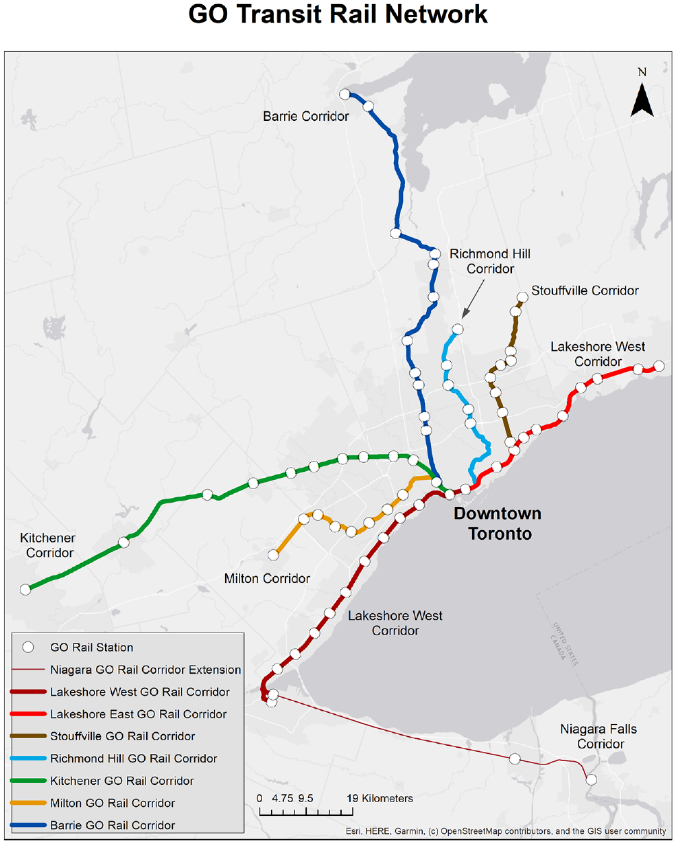
Schematic diagram of GO Transit rail network in Ontario, Canada.

Station access to the system is primarily facilitated by private automobile, as 62% of riders access the station via this mode. A total of 61 stations throughout the study area have some type of park and ride infrastructure that customers can utilize. Alternative access options, such as feeder bus connections, are also provided by local transit service providers.

Modeling Framework

The purpose of this research is to estimate the sensitivity of existing GO Transit demand to various service and demographic variables, such that estimates can be generated on ridership after the planned transition from a commuter to a regional system. The data for the model include four general categories: estimates of the quantity and extent of services provided by GO Transit; representations of the socioeconomic and demographic attributes of those within the catchment areas of the existing network; factors specific to the local context of the service area, such as station accessibility indicators; and the station-level ridership (boardings) throughout the network. As described in the following sections, these data can be considered “panel data”, where the same station-level variables are observed over subsequent time periods.

Pooled ordinary least squares (OLS) is a simplistic approach used when panel data is modeled, where a simple OLS regression is run on all observations. However, since spatial and temporal relationships are not controlled for, this method is rarely used to produce final outputs and is instead used as a baseline to introduce advanced modeling frameworks ( 7 ).

To improve model performance with panel data, fixed effect models are often considered. This approach assumes that each entity (station) has its own individual characteristics that could influence the dependent variable, and therefore need to be controlled ( 7 ). Time-invariant characteristics and the effect of these variables are removed, and instead are captured in the unknown intercept of each entity. The model also assumes that the entity’s error term and its independent variables are correlated. Therefore, a fixed effect estimator is only concerned with analyzing change in the dependent variable attributed to temporal variation in the independent factors. As shown in Equation 1, the model takes the following form:

γ_{it} = β_{1} x_{it 1} + β_{2} x_{it 2} +_{\dots} β_{k} x_{itk} + a_{i} + u_{it}

(1)

where:

$γ_{it}$ = the dependent variable,

$x_{itk}$ accounts for the factors included in the analysis,

$β_{k}$ = the slope estimate for a given independent variable,

$a_{i}$ controls for the unobserved fixed effects for each entity, and

$u_{it}$ = the model’s idiosyncratic error term.

A random effect model can be used if the idiosyncratic error term is assumed to be uncorrelated with associated independent variables ( 7 ). Therefore, time-invariant variables can be included in this estimator, but entity-specific characteristics that could influence the dependent variable need to be controlled for to ensure that the analyzed effects are truly random. As shown in Equation 2, the random effect model takes the following form:

γ_{it} = β_{1} x_{it 1} + β_{2} x_{it 2} +_{\dots} β_{k} x_{itk} + a + u_{it} + ε_{it}

(2)

where:

$a$ = the intercept of the model,

$u_{it}$ controls for the combined time-series and cross-sectional error, and

$ε_{it}$ = the individual specific cross-sectional error terms.

When selecting the appropriate estimator, it is common practice to analyze the panel dataset using both pooled OLS, fixed effect, and random effect models. Statistical tests are then applied to model outputs to determine the method that best suits the dataset. This is the approach taken in this research.

Data Collection

This section describes the data that were gathered for the analysis and, where appropriate, assumptions made in creating data sets for the models.

Station Selection

Ridership data were collected at the station-level at monthly intervals from January 2016 to December 2019, resulting in 48 observation periods. This temporal scale (i.e., four years) was selected to ensure that both short and long run demand effects could be accounted for in the modeling framework. A total of 68 stations along all GO corridors were initially considered for inclusion. Several stations that became operational during the time-series were excluded to ensure that the effects of network expansion were not captured in the analysis. Union Station was also excluded, as heightened ridership figures experienced at this station would have produced skewed model outputs. After these adjustments were made, 61 stations were included in the analysis.

Dependent Variable

Station-level weekday boardings as indicated by the PRESTO system were used to formulate the dependent variable dataset. Weekend boardings were excluded from the analysis, as limited service offerings were provided during these time periods. To control for trip type/purpose, filters were applied so that counts could be separated by different time periods: a.m. peak (05:00–09:30), midday off-peak (09:31–14:59), p.m. peak (15:00–19:00), and evening off-peak (19:01–end of service). Observations were only considered if outbound service was offered, to (1) ensure that the station was operational during the time-series analyzed, and (2) ensure that a corresponding ridership count was available for analysis. All stations in the study area offer outbound service during the a.m. peak period; therefore, all 61 stations were included in the a.m. peak analysis. Fewer stations were included in the remaining models, as two-way, all-day service is currently only provided to stations located along the Lakeshore corridors. Since GO ridership is primarily comprised of commuters, it was theorized that monthly variation in the number of business days could influence monthly boardings. Ridership figures were therefore normalized by the number of business days in each month to account for these differences.

Estimation of Station Catchment Areas

Datasets that captured regional geography, metropolitan economy, and population characteristics were compiled using overlay analysis. To ensure that these statistics were representative of the current demand pool, customer origin records were used to formulate station catchment areas around each station included in the analysis.

PRESTO data, indicating the postal code of the customer’s home address, access station, and number of trips generated by the user, were obtained for the duration of the time series. A shapefile illustrating the residential location of each customer was digitized using ArcMap software. Following the methodology outlined by Engel-Yan et al., all customer origin records located farther than 10 kilometers from the access station were eliminated to ensure that only home-based trips were included in the analysis ( 19 ). A heatmap weighted to the number of trips generated by each remaining user was then created, highlighting areas with the greatest concentration of transit activity (Figure 2). A polygon was then digitized around the heatmap and exported as the corresponding station catchment area.

Figure 2.

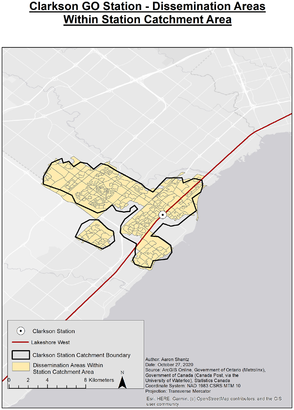
Example of process used to delineate station catchment areas and extract corresponding external variable datasets.

Independent Variables

As described in the literature review, several independent variables are known to influence the propensity to use transit. Among these, those capturing factors both internal (i.e., fare price) and external (i.e., demographic indicators) to the transit agency were used in the current study. Data about population density, employment density, gender, income, unemployment rate, age, and count data representing the number of children per household were downloaded from the 2006, 2011, and 2016 Canadian Census of Population. In some cases, values were also obtained from the 2011 National Household Survey. Collected at the dissemination area scale, extrapolation was used to estimate unique monthly values, ensuring that changing demographic and socioeconomic trends could be accounted for in the modeling process. If observations could not be obtained from all three census products, values obtained from the 2016 census were used to fill values throughout the time series. Once completed, GIS tools were used to extract observations at the station-level using the station catchment areas previously estimated.

Observations were collected for several additional factors, including those specific to the local context such as station-level park and ride capacity (Table 1). Refer to Shantz for a complete description of methods used to compile and process each dataset ( 23 ).

Table 1.

Description of Factors Included in Analysis

Variable	Indicator	Type of data	Data source/spatial scale (if applicable)	Are values time-variant?	Unique values obtained for different trip types?
Ridership	Average daily number of boardings	Continuous	PRESTO server	Yes	Yes
Population density	Population density	Continuous	Census products, dissemination area	Yes, unique values obtained via extrapolation	No
Employment density	Density of incoming commuters	Continuous	Census products, census tract	No	No
Gender: female	Percentage of population female	Continuous	Census products, dissemination area	Yes, unique values obtained via extrapolation	No
Income	Median household income	Continuous	Census products, dissemination area	Yes, unique values obtained via extrapolation	No
Unemployment rate	Unemployment rate	Continuous	Census products, dissemination area	Yes, unique values obtained via extrapolation	No
Age	Median age	Continuous	Census products, dissemination area	Yes, unique values obtained via extrapolation	No
Households with children	Density of households with children	Continuous	Census products, dissemination area	Yes, unique values obtained via extrapolation	No
Vehicle availability/ownership	Total amount of private vehicles owned	Continuous	Transportation tomorrow survey, upper/single-tier municipality	Yes, unique values obtained via extrapolation	No
Fuel price	Price of 1 liter of unleaded fuel	Continuous	Ontario fuel price survey, region relative to City of Toronto	Yes, unique monthly observations available for duration of time-series	No
Service quantity	Number of outbound trips per station	Continuous	Generalized transit feed specification files	Yes, unique monthly observations available for duration of time-series	Yes
Fare price	Average fare price	Continuous	PRESTO server	Yes, unique monthly observations available for duration of time-series	Yes
Distance to central business district: near	Station located within City of Toronto	Nominal	Metrolinx open data portal	Yes, unique monthly observations available for duration of time-series	No
Distance to central business district: far	Station not located within City of Toronto	Nominal	Metrolinx open data portal	Yes, unique monthly observations available for duration of time-series	No
Number of parking spaces	Total number of parking spaces	Continuous	Metrolinx open data portal	Yes, unique monthly observations available for duration of time-series.	No
Feeder bus connection quality	Average transit access time	Continuous	Generalized transit feed specification files	Yes, unique monthly observations available for duration of time-series	Yes
Winter	Observation occurred in January, February, or March	Nominal	na	No	No
Spring	Observation occurred in April, May, or June	Nominal	na	No	No
Summer	Observation occurred in July, August, or September	Nominal	na	No	No
Fall	Observation occurred in October, November, or December	Nominal	na	No	No

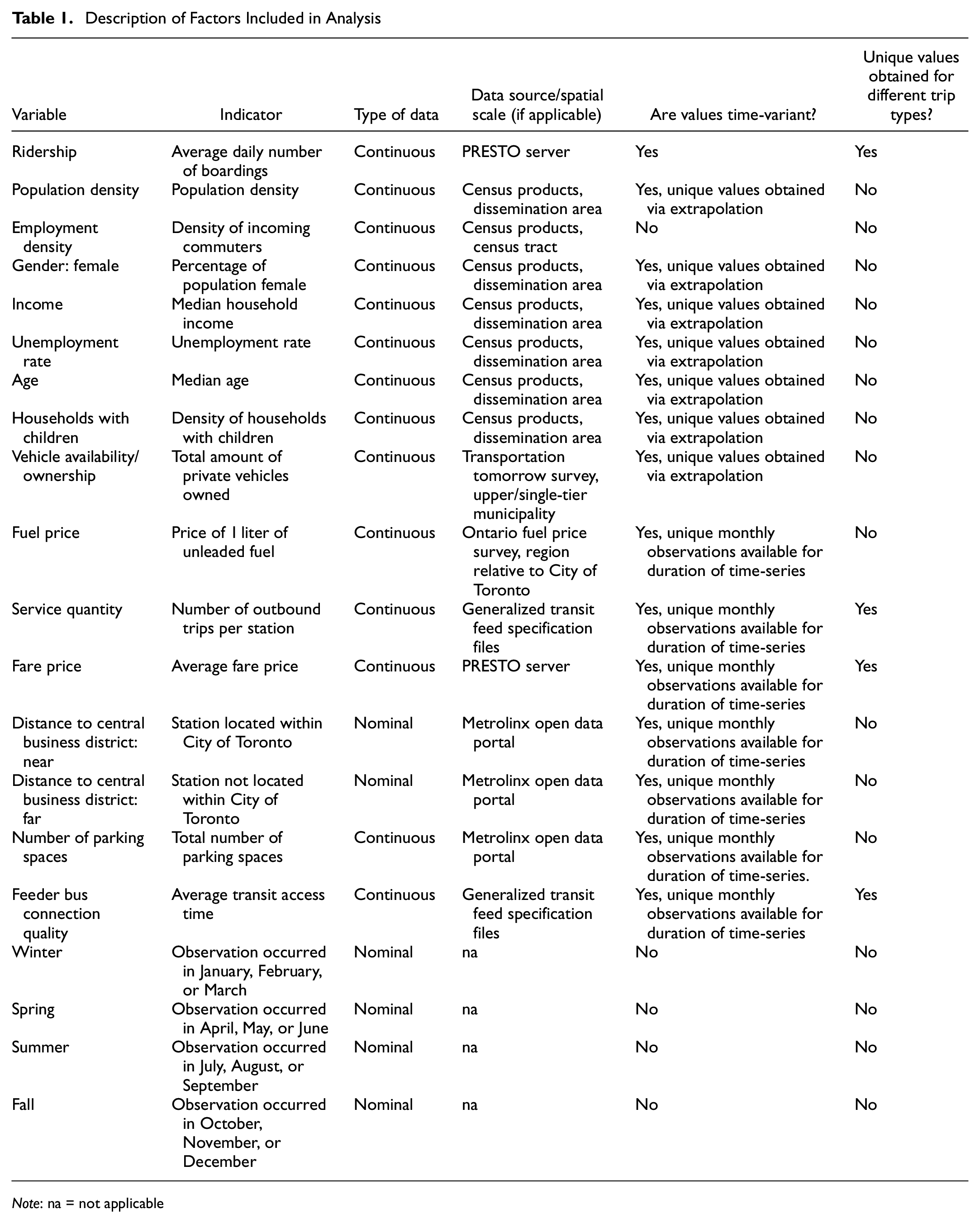
Note: na = not applicable

Data Analysis

As with any data set, this research required some modifications to and assessments of the input data to enhance the model’s performance. To account for inflation, variables including fare price, income, and fuel price were converted to January 2016 Canadian dollars using Canada’s Consumer Price Index. All continuous variables were also transformed by their natural logarithm so that estimated coefficients could be directly interpreted as ridership elasticities ( 5 , 6 ). To control for multi-collinearity, variables demonstrating a correlation coefficient greater than 0.85 were removed (only one variable was selected), and it was ensured that the variance inflation factor (VIF) of each independent variable did not exceed 10.

Various modeling approaches, including pooled OLS, fixed effect, and random effect estimators, were initially considered. Using a Breusch-Pagen Lagrange multiplier test, significant results were found when the fixed and random effect models were compared with the pooled OLS estimator, indicating the presence of time and entity effects. A random effect estimator was selected to produce the final model outputs so demand could be explained by both cross-sectional, temporal, and time-invariant factors.

Each model was then tested for the presence of heteroskedasticity and serial correlation of error terms using Durbin-Watson and Breusch-Pagen tests. Model outputs were estimated with White robust standard errors, clustered at the station-level, to control for these effects.

A backwards stepwise regression was used to eliminate insignificant independent variables from each model. This was completed by selecting and eliminating the independent variable associated with the largest p-value in each model. Once a variable was removed, model outputs were recalculated so that updated results could further inform the stepwise process. This continued until all variables included in each model were statistically significant, evidenced by a corresponding p-value less than or equal to 0.1.

Results

Model Fit

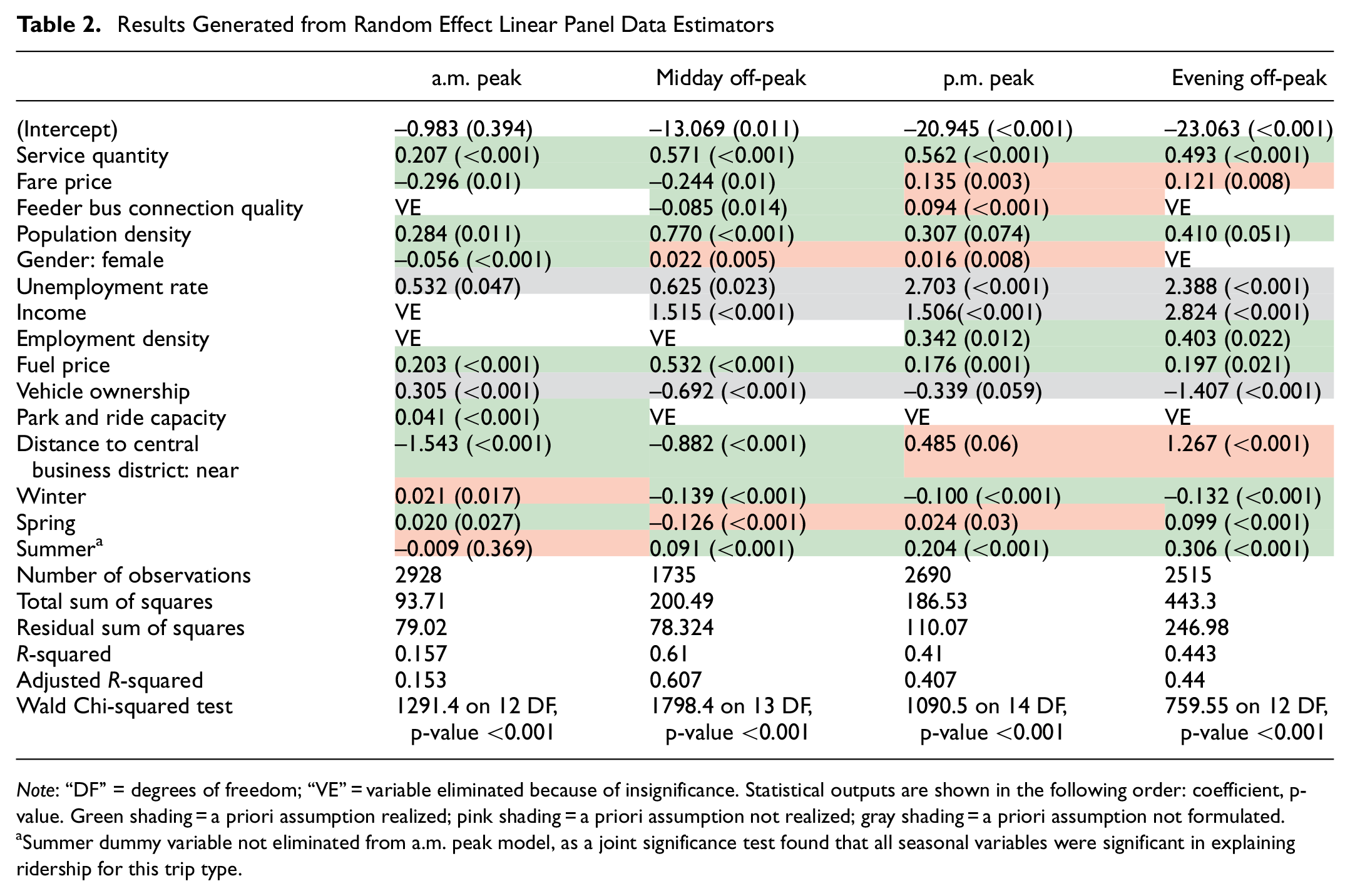
Results and associated demand elasticity estimates are summarized in Table 2. Wald’s Chi-squared tests of overall significance returned significant results for each model, indicating that the dependent variable was significantly affected by the independent variables selected. The R-squared test statistic found that the explanatory capacity of the a.m. peak model was significantly less than the other models estimated, although this can be explained by the spread and range of station-level ridership during this period relative to the other trip types examined. Random influences including the opening/closing of local businesses, construction, and special events could have further contributed to these trends ( 24 ).

Table 2.

Results Generated from Random Effect Linear Panel Data Estimators

	a.m. peak	Midday off-peak	p.m. peak	Evening off-peak
(Intercept)	–0.983 (0.394)	–13.069 (0.011)	–20.945 (<0.001)	–23.063 (<0.001)
Service quantity	0.207 (<0.001)	0.571 (<0.001)	0.562 (<0.001)	0.493 (<0.001)
Fare price	–0.296 (0.01)	–0.244 (0.01)	0.135 (0.003)	0.121 (0.008)
Feeder bus connection quality	VE	–0.085 (0.014)	0.094 (<0.001)	VE
Population density	0.284 (0.011)	0.770 (<0.001)	0.307 (0.074)	0.410 (0.051)
Gender: female	–0.056 (<0.001)	0.022 (0.005)	0.016 (0.008)	VE
Unemployment rate	0.532 (0.047)	0.625 (0.023)	2.703 (<0.001)	2.388 (<0.001)
Income	VE	1.515 (<0.001)	1.506(<0.001)	2.824 (<0.001)
Employment density	VE	VE	0.342 (0.012)	0.403 (0.022)
Fuel price	0.203 (<0.001)	0.532 (<0.001)	0.176 (0.001)	0.197 (0.021)
Vehicle ownership	0.305 (<0.001)	–0.692 (<0.001)	–0.339 (0.059)	–1.407 (<0.001)
Park and ride capacity	0.041 (<0.001)	VE	VE	VE
Distance to central business district: near	–1.543 (<0.001)	–0.882 (<0.001)	0.485 (0.06)	1.267 (<0.001)
Winter	0.021 (0.017)	–0.139 (<0.001)	–0.100 (<0.001)	–0.132 (<0.001)
Spring	0.020 (0.027)	–0.126 (<0.001)	0.024 (0.03)	0.099 (<0.001)
Summer^a	–0.009 (0.369)	0.091 (<0.001)	0.204 (<0.001)	0.306 (<0.001)
Number of observations	2928	1735	2690	2515
Total sum of squares	93.71	200.49	186.53	443.3
Residual sum of squares	79.02	78.324	110.07	246.98
R-squared	0.157	0.61	0.41	0.443
Adjusted R-squared	0.153	0.607	0.407	0.44
Wald Chi-squared test	1291.4 on 12 DF, p-value <0.001	1798.4 on 13 DF, p-value <0.001	1090.5 on 14 DF, p-value <0.001	759.55 on 12 DF, p-value <0.001

Note :“DF” = degrees of freedom; “VE” = variable eliminated because of insignificance. Statistical outputs are shown in the following order: coefficient, p-value. Green shading = a priori assumption realized; pink shading = a priori assumption not realized; gray shading = a priori assumption not formulated.

Summer dummy variable not eliminated from a.m. peak model, as a joint significance test found that all seasonal variables were significant in explaining ridership for this trip type.

Notable Findings

Service quantity was positively associated with ridership in all models, as elasticities ranging from 0.207 to 0.571 were calculated. This supports the supposition that increasing service stimulates demand regardless of travel purpose ( 4 , 6 , 25 ). Demand during the a.m. peak period was least responsive to service quantity, although this could be explained by extensive baseline service already offered ( 12 , 15 , 17 ). These findings suggest that commuter rail demand should increase as service expansions are implemented, but marginal gains may be realized as customers become acclimatized to adequate service levels.

Fare price elasticities ranged between −0.296 and 0.135, while a negative correlation was only found by the a.m. peak and midday off-peak models. Various studies have suggested that a lack of parking in the study area’s central business district (CBD), high parking costs experienced at employment destinations, and/or marginal change in the fare price variable can result in underestimated fare price elasticities ( 26 ). Through policy review, it was further identified that fare price changes experienced throughout the time-series were not uniform in direction, as fare prices were increased for long-distance trips, while those 10 kilometers or less in length were reduced to a flat rate of $3.70. While these aspects may explain why fare price elasticities were less compared with those associated with other internal factors, they do little to explain why a positive correlation was shown in the p.m. peak and evening off-peak periods. Likely, alternative metrics, further research, or both, is needed to accurately assess the impact of zonal/distance-based fare price changes on commuter rail demand patterns.

Population density demonstrated a positive relationship with ridership in all models, as elasticities ranging from 0.284 to 0.77 were found. Consistent with previous studies, the results suggest that rail demand can be increased significantly when dense developments are constructed close to the network ( 11 , 14 , 25 ). Further to Miller et al., heightened elasticities estimated by the off-peak models suggests that discretionary demand is more sensitive to increased population densities instead of commuter related trips ( 24 ). However, since key trips generated in the a.m. peak period are disproportionally located in sprawled suburban areas, the magnitude of this relationship could have been minimized.

Employment density demonstrated a positive correlation with transit demand, but only during the p.m. peak and evening off-peak periods. This conforms to the expectation that most travel is work based during these periods as commuters return to residential areas. The comparable sign and significance of population density within these models suggests that the presence of mixed land uses is a key driver of station-level demand; these uses often generate more discretionary traffic as a result of late operating hours and recreational offerings ( 11 , 12 ). The implementation of diverse land use planning policies around commuter rail stations could effectively increase demand during the latter half of the day.

Unemployment rate demonstrated a positive relationship with demand in each model. Although consistent with results identified by Stover and Christine Bae, the extrapolation methodology used to obtain unemployment rate values could explain this finding ( 10 , 27 ). Since highly variable industrial and economic trends could not be captured in this dataset, these values were most likely misspecified, thus resulting in a skewed understanding of the sign and significance of this relationship.

Station location was significantly associated with ridership. Stations near the study area’s CBD were associated with fewer boardings during the a.m. peak and midday off-peak periods, while the opposite relationship was identified in the p.m. peak and evening off-peak models. Spatial dependencies were expected, as commuter rail users typically reside in suburban locations and commute to downtown employment centres. However, the magnitude of these relationships suggests that additional aspects not included in the modeling process limit the use of the system for inter-city travel.

Seasonality was shown to have a significant impact on demand in all time periods. Using fall as a baseline, observations that occurred during the winter demonstrated a negative correlation with demand, while ridership increased in summer months. Inadequate station infrastructure could be a driver of decreased winter ridership, as being exposed to cold weather and precipitation events may encourage choice riders to use private automobile ( 28 ). Changes to station infrastructure, such as the number of heated shelters and the amount of indoor seating, could further deter these impacts ( 29 ).

Park and ride capacity was associated with more boardings, but only during the a.m. peak period. A demand elasticity of 0.041 further suggests that ridership is not overly sensitive to increased parking capacity. The demand relationship is likely minimized as: (1) minimal parking expansion occurred throughout the time-series analyzed, and (2) ridership is proportionally concentrated at stations with large parking facilities (i.e., Oakville GO Station), and those where station access is primarily facilitated by active transport modes (i.e., Exhibition GO Station). This indicates that the presence of park and ride facilities has enabled ridership figures to this point, but further parking expansion is not needed to encourage new demand. Further research could instead measure how transport behavior responds to variation in parking utilization, rather than parking capacity, as uncertainty about parking availability could influence station-level demand patterns.

Similar to parking capacity, feeder bus connection quality does little to explain station-level ridership throughout the study area. The expected sign was only displayed during the midday off-peak period, while a marginal coefficient of −0.085 suggests that demand is relatively unaffected when poor connections are provided. This could be explained by the presence of indirect routes, large headways, and dispersed service coverage that is common of local transit providers that operate throughout the GGH.

The price of fuel significantly explained ridership, as elasticities greater than 0.176 were found in all models. The significance of these results indicate that push techniques aimed at increasing the disutility of private automobile use is a viable method to increase demand ( 6 , 16 ).

More vehicles were associated with increased ridership during the a.m. peak period, while the opposite relationship was identified for the remaining trip types examined. Consistent with Balcombe et al., these findings were expected, as the utility generated by increased productivity can influence automobile owners to use the system for part of their journey ( 4 ). Significant congestion in and around the city of Toronto during the a.m. peak period can further explain this relationship, as increased travel times, unreliability, and reduced productivity increase the utility associated with rail use compared with private automobile use. The remaining models indicate that private automobile availability is a competitive good that negatively affects ridership in other time periods. This may be a result of improved traffic conditions commonly realized once the a.m. peak period concludes, meaning that the disutility otherwise associated with private automobile use is reduced. These findings further suggest that policies which disincentivize automobile use during most time periods could encourage the use of commuter rail systems.

Policy Implications and Conclusions

This study sought to identify factors significantly associated with GO Transit commuter rail ridership. Independent variable datasets, including those related to the study area’s regional geography, economy, population characteristics, transit system aspects, and the surrounding automobile/highway system, were collected across a 48-month time-series. Datasets were separated into a.m. peak, midday off-peak, p.m. peak, and evening off-peak periods to determine if relationships differed depending on trip type analyzed. A random effect linear panel data estimator was then used to determine the explanatory power of each variable. The results revealed that ridership was consistently influenced by service quantity, population density, fuel price, and station location. Notably, the sign and significance of fare price, park and ride capacity, feeder bus connection quality, and vehicle ownership differed between models. This study highlights the importance of disaggregating demand elasticity estimates by trip type, as policies targeted toward stimulating demand in all time periods should be prioritized to encourage ridership growth. As summarized in Table 3, the findings indicate that a variety of planning policies, in addition to service quantity improvements outlined in the GO Expansion Program, could be implemented to stimulate commuter rail demand.

Table 3.

Key Findings and Associated Policy Implications

Variable	Relationship with demand^a				Interpretation of finding	Policy implications
Service quantity	+	+	+	+	Ridership stimulated when convenient, accessible, and high-quality transit options provided.	Continue with planned service expansions.
Fuel price	-	-	-	-	Auto operation costs disincentivize use, and increase transit ridership.	Implement transport pricing schemes including fuel/parking taxes, road tolls and congestion charges.
Vehicle ownership	+	-	-	-	Vehicle ownership competitive good to commuter rail.
Population density	+	+	+	+	Ridership more likely when dense developments located near commuter rail stations.	Stimulate transit-oriented development via minimum density targets.
Employment density	NA	NA	+	+	Ridership more likely when jobs/employment uses located near commuter rail stations.	Stimulate transit-oriented development via mixed land use designations.
Distance to central business district: near	-	-	+	+	Inter-city ridership restricted by price/availability of conventional transit options.	Implement integrated and competitive fare options for inter-city travelers.
Seasonality (winter)	+	-	-	-	Disutility of cold weather, precipitation discourages commuter rail demand.	Upgrade station infrastructure including heated shelters, indoor seating, and covered platforms.
Park and ride capacity	+	NA	NA	NA	Commuter rail demand unresponsive to increased park and ride capacity.	Avoid costly expansions of park and ride infrastructure, investigate alternative first-and-last-mile solutions.

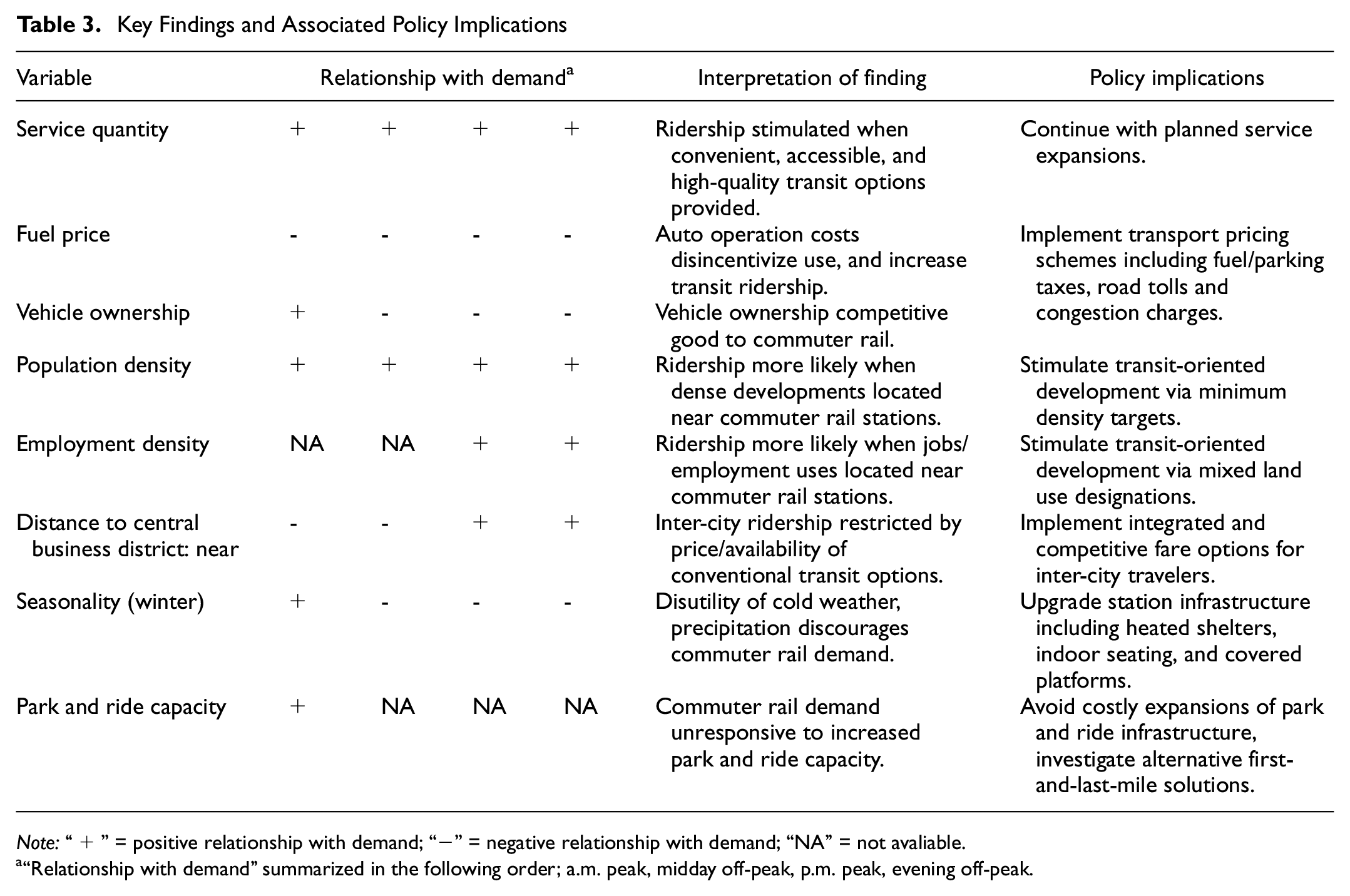
Note:“+” = positive relationship with demand; “−” = negative relationship with demand; “NA” = not avaliable.

“Relationship with demand” summarized in the following order; a.m. peak, midday off-peak, p.m. peak, evening off-peak.

The explanatory power associated with population density suggests that the development of dense, residential settlements near commuter rail networks could be a significant driver of ridership. The joint significance of employment density in the p.m. peak and evening off-peak periods further indicates that the implementation of transit supportive land use policies could be more effective. However, the GO Expansion Program is not accompanied by a formal development strategy to support this initiative.

Instead, the GO Expansion Program refers to provincial planning guidelines to guide growth throughout the study area. Of these, the regional growth plan for the GGH states that lands surrounding GO Transit stations should be zoned for mixed-use development, and mandates these areas should be zoned for a minimum density of 150 residents and jobs combined per hectare to ensure that these areas are transit supportive ( 22 ). However, a desktop review found that these guidelines are only required for 37 stations throughout the study area. Further, few municipalities subjected to these guidelines have implemented these policies in formal, municipal-level planning policies. Consistent with Chen and Zegras, the results of this study suggest that a consistent and encompassing transit-oriented development policy should be developed in conjunction with rail expansion plans, to ensure that residents and employment are concentrated near to the network ( 12 ).

The significant correlation with fuel price suggests that demand is associated with vehicle operation costs. Comparative studies have found that the availability and price of parking is the most significant variable that influences the utility of automobile use ( 30 , 31 ). Specifically, researchers have identified that mode shift occurs most frequently when a tax on parking space use is implemented. Further, several studies have found that pricing mechanisms, such as congestion charges, road pricing, and road tolls, can have similar impacts on demand ( 32 , 33 ). Therefore, similar pricing mechanisms could be implemented within major North American cities to transition private automobile users to commuter rail networks.

Finally, the results of this study found that distance to the CBD had a significant impact on station-level demand in all time periods examined. Previous studies have theorized that the price, abundance, and accessibility of local transit service available within major urban areas can explain these trends. A study of New Jersey Transit’s commuter rail system found that system uptake is less likely when extensive transit options are already available to the customer, while Hensher found that rail demand can increase when conventional transit providers increase fares ( 28 , 34 ). Balcombe et al. also suggested that metro ridership is associated with the price of alternatives, as a 0.18 demand elasticity with respect to rail fares was found ( 4 ). These results illustrate that commuter rail demand could be negatively affected if inexpensive or more convenient transit options are available to users.

While cross-elasticities were not directly measured as part of this study, a review of alternative transit options and associated fare price schemes found this to be a plausible explanation. Conventional transit providers within the study area charge a flat fare of $3.25 for all trips, while the price of a trip between GO rail stations in the city of Toronto was approximately 86% higher. Therefore, inter-city travelers are most likely to select conventional services, as the disutility of use is substantially less. The findings highlight the importance of integrated and competitive fare pricing options to increase competitiveness with other transit providers, balance network utilization, and increase overall ridership figures.

The results of this study amplify those found in recent demand elasticity studies, further suggesting that a variety of factors are significantly associated with commuter rail demand ( 11 , 12 , 25 ). Therefore, policies centered around service quantity expansions, such as the GO Expansion Program, are a viable method of increasing ridership in the North American context. Complementary policies that mandate the implementation of mixed-use developments, increase the cost of vehicle operation, and regulate the cost of system use are also needed if substantial mode shift is expected. Future research could be undertaken that utilizes a multi-city approach and broader cross-section of commuter rail transit agencies to further understand the main determinants of commuter rail ridership across varying geographies. Until then, this work can be extended to other regional transit agencies currently engaged in commuter to regional rail transition, and highlights the importance of integrated planning policies when considering such conversions.

Footnotes

Acknowledgements

The authors would like to thank Metrolinx for their assistance via the 2020 Rob MacIsaac Fellowship Program; Service Planning staff for providing fare price and customer origin statistics; and Eddy Ionescu for his assistance processing service quantity data.

Author Contributions

The authors confirm contribution to the paper as follows: study conception and design: A. Shantz, J. Casello, C. Woudsma; data collection: A. Shantz, J. Casello, C. Woudsma; analysis and interpretation of results: A. Shantz, J. Casello, C. Woudsma; draft manuscript preparation; A. Shantz, J. Casello, C. Woudsma, E. Guerra. All authors reviewed the results and approved the final version of the manuscript.

Declaration of Conflicting Interests

The author(s) declared no potential conflicts of interest with respect to the research, authorship, and/or publication of this article.

Funding

The author(s) disclosed receipt of the following financial support for the research, authorship, and/or publication of this article: This work was supported by the Government of Ontario (via Metrolinx), through the 2020 Rob MacIsaac Fellowship Program.

ORCID iDs

Aaron Shantz

Jeff Casello

Clarence Woudsma

Data Accessibility Statement

The data that support the findings of this study are available from the corresponding author, A. Shantz, on reasonable request.

References

Newman

P. W. G.

Kenworthy

J. R.

The Land Use-Transport Connection: An Overview. Land Use Policy, Vol. 13, No. 1, 1996, pp. 1–22. https://doi.org/10.1016/0264-8377(95)00027-5.

Vuchic

V. R.

Urban Transit Systems and Technology. John Wiley & Sons, Hoboken, NJ, 2007. https://doi.org/10.1002/9780470168066.

Ingvardson

J. B.

Nielsen

O. A.

How Urban Density, Network Topology and Socio-Economy Influence Public Transport Ridership: Empirical Evidence From 48 European Metropolitan Areas. Journal of Transport Geography, Vol. 72, 2018, pp. 50–63. https://doi.org/10.1016/j.jtrangeo.2018.07.002.

Balcombe

Mackett

Paulley

Preston

Shires

Titheridge

Wardman

White

The Demand for Public Transport: A Practical Guide. Transport Policy, Vol. 13, No. 4, 2004, 295–306.

Holmgren

Meta-analysis of Public Transport Demand. Transportation Research Part A: Policy and Practice, Vol. 41, No. 10, 2007, pp. 1021–1035. https://doi.org/10.1016/j.tra.2007.06.003.

Taylor

B. D.

Miller

Iseki

Fink

Nature and/or Nurture? Analyzing the Determinants of Transit Ridership Across US Urbanized Areas. Transportation Research Part A: Policy and Practice, Vol. 43, No. 1, 2009, pp. 60–77. https://doi.org/10.1016/j.tra.2008.06.007.

Wooldridge

J. M.

Introductory Econometrics - A Modern Approach, 5th ed. Cengage Learning, South-Western, 2012. https://economics.ut.ac.ir/documents/3030266/14100645/Jeffrey_M._Wooldridge_Introductory_Econometrics_A_Modern_Approach__2012.pdf.

Curtin

J. F.

Effect of Fares on Transit Riding. Highway Research Record 213. HRB, National Research Council, Washington, D.C., 1968, pp. 8–20.

Schimek

Dynamic Estimates of Fare Elasticity for U.S. Public Transit. Transportation Research Record: Journal of the Transportation Research Board, 2015. 2538: 96–101. https://doi.org/10.3141/2538-11.

10.

Stover

V. W.

Christine Bae

C. H.

Impact of Gasoline Prices on Transit Ridership in Washington State. Transportation Research Record: Journal of the Transportation Research Board, 2011. 2217: 11–18. https://doi.org/10.3141/2217-02.

11.

Durning

Townsend

Direct Ridership Model of Rail Rapid Transit Systems in Canada. Transportation Research Record: Journal of the Transportation Research Board, 2015. 2537: 96–102. https://doi.org/10.3141/2537-11.

12.

Chen

S. H.

Zegras

Rail Transit Ridership: Station-area Analysis of Boston’s Massachusetts Bay Transportation Authority. Transportation Research Record: Journal of the Transportation Research Board, 2016. 2544: 110–122. https://doi.org/10.3141/2544-13.

13.

Liu

Erdogan

Ducca

F. W.

How to Increase Rail Ridership in Maryland: Direct Ridership Models for Policy Guidance. Journal of Urban Planning and Development, Vol. 142, No. 4, 2016, P. 04016017. https://doi.org/10.1061/(asce)up.1943-5444.0000340

14.

Brown

Thompson

Bhattacharya

Jaroszynski

Understanding Transit Ridership Demand for the Multidestination, Multimodal Transit Network in Atlanta, Georgia: Lessons for Increasing Rail Transit Choice Ridership while Maintaining Transit Dependent Bus Ridership. Urban Studies, Vol. 51, No. 5, 2014, pp. 938–958. https://doi.org/10.1177/0042098013493021.

15.

Wasserman

A Time and a Place for Every Rider? Geographic and Temporal Changes in Bay Area Transit Ridership. Institute of Transportation Studies, Los Angeles, CA, 2019. https://doi.org/10.17610/T6KW22.

16.

Lane

B. W.

A Time-series Analysis of Gasoline Prices and Public Transportation in US Metropolitan Areas. Journal of Transport Geography, Vol. 22, 2012, pp. 221–235. https://doi.org/10.1016/j.jtrangeo.2011.10.006.

17.

Yanmaz-Tuzel

Ozbay

Impacts of Gasoline Prices on New Jersey Transit Ridership. Transportation Research Record: Journal of the Transportation Research Board, 2010. 2144: 52–61. https://doi.org/10.3141/2144-07.

18.

Guerra

Cervero

Tischler

Half-Mile Circle Does It Best Represent Transit Station Catchments?

Transportation Research Record: Journal of the Transportation Research Board, 2012. 2276: 101–109.

19.

Engel-Yan

Rudra

Livett

Nagorsky

Strategic Station Access Planning for Commuter Rail Balancing Park-and-Ride With Other Modes. Transportation Research Record: Journal of the Transportation Research Board, 2014. 2419: 82–91. https://doi.org/10.3114/2419-08.

20.

Government of Ontario. A Place to Grow – Growth Plan for the Greater Golden Horseshoe, Office Consolidation. Government of Ontario, Toronto, ON, 2020. https://doi.org/978-1-4868-4654-2.

21.

Ashby

Transportation Tomorrow Survey 2016: 2016, 2011, 2006, 2001, 1996 and 1986 Travel Summaries for the TTS Area, 2018. http://dmg.utoronto.ca/pdf/tts/2016/2016TTS_Summaries_TTSarea.pdf.

22.

Government of Ontario. GO Expansion Full Business Case, 2018. http://www.metrolinx.com/en/docs/pdf/board_agenda/20181206/20181206_BoardMtg_GO_Expansion_Full_Business_Case.PDF.

23.

Shantz

Understanding Factors Associated With Commuter Rail Ridership - A Demand Elasticity Study of the GO Transit Rail Network. UWSpace, 2021. http://hdl.handle.net/10012/16950.

24.

Miller

Savage

Does the Demand Response to Transit Fare Increases Vary by Income?

Transport Policy, Vol. 55, 2017, pp. 79–86. https://doi.org/10.1016/j.tranpol.2017.01.006.

25.

Guerra

Cervero

Cost of a Ride. Journal of the American Planning Association, Vol. 77, No. 3, 2011, pp. 267–290. https://doi.org/10.1080/01944363.2011.589767.

26.

Kohn

Factors Affecting Urban Transit Ridership. Statistics Canada, Archived Journals and Periodicals, 53F0003-XI, 2000, pp. 271–285. https://www150.statcan.gc.ca/n1/en/catalogue/53F0003X.

27.

Weden

M. M.

Peterson

C. E.

Miles

J. N.

Shih

R. A.

Evaluating Linearly Interpolated Intercensal Estimates of Demographic and Socioeconomic Characteristics of U.S. Counties and Census Tracts 2001–2009. Population Research and Policy Review, Vol. 34, No. 4, 2015, pp. 541–559. https://doi.org/10.1007/s11113-015-9359-8.

28.

Chen

Varley

Chen

What Affects Transit Ridership? A Dynamic Analysis Involving Multiple Factors, Lags and Asymmetric Behaviour. Urban Studies, Vol. 48, No. 9, 2011, pp. 1893–1908. https://doi.org/10.1177/0042098010379280.

29.

Singhal

Kamga

Yazici

Impact of Weather on Urban Transit Ridership. Transportation Research Part A: Policy and Practice, Vol. 69, 2014, pp. 379–391. https://doi.org/10.1016/j.tra.2014.09.008.

30.

Morrall

Bolger

Relationship Between Downtown Parking Supply and Transit Use. ITE Journal, Vol. 66, No. 2, 1996, p. 32.

31.

Bianco

M. J.

Dueker

Strathman

J. G.

Parking Strategies to Attract Auto Users to Public Transportation, 1997. http://pdxscholar.library.pdx.edu/cus_pubs/33?utm_source=pdxscholar.library.pdx.edu%2Fcus_pubs%2F33&utm_medium=PDF&utm_campaign=PDFCoverPages

32.

Arentze

Hofman

Timmermans

Predicting Multi-Faceted Activity-Travel Adjustment Strategies in Response to Possible Congestion Pricing Scenarios Using an Internet-based Stated Adaptation Experiment. Transport Policy, Vol. 11, No. 1, 2004, pp. 31–41. https://doi.org/10.1016/S0967-070X(03)00016-7.

33.

U.S. Department of Transportation. Congestion Pricing—A Primer: Overview, 2008. https://ops.fhwa.dot.gov/publications/fhwahop08039/fhwahop08039.pdf.

34.

Hensher

D. A.

Establishing a Fare Elasticity Regime for Urban Passenger Transport. Journal of Transport Economics and Policy, Vol. 32, No. 2, 1998, pp. 221–246. https://www.jstor.org/stable/20053767.

Understanding Factors Associated with Commuter Rail Ridership: A Demand Elasticity Study of the GO Transit Rail Network

Abstract

Keywords

Literature Review

Demand Elasticity Methods

Factors Associated with Demand

Delineating Station Catchment Areas

Literature Gaps

Methods

Study Area

Modeling Framework

Data Collection

Station Selection

Dependent Variable

Estimation of Station Catchment Areas

Independent Variables

Data Analysis

Results

Model Fit

Notable Findings

Policy Implications and Conclusions

Footnotes

Acknowledgements

Author Contributions

Declaration of Conflicting Interests

Funding

ORCID iDs

Data Accessibility Statement

References