Sage Journals: Discover world-class research

Abstract

Bridge deck deterioration modeling is critical to infrastructure management. Deterioration modeling is traditionally done using deterministic models, stochastic models, and recently basic machine learning methods. The advanced machine learning-based survival models, such as random survival forest, have not been adapted for use in infrastructure management. This paper introduces random survival forest models for bridge deck deterioration modeling and compare their performance with a commonly used traditional stochastic model, that is, the Weibull distribution-based accelerated failure time (AFT-Weibull) model. To better adapt the random survival model for bridge deck deterioration modeling, the selection of the dependent variables is discussed between two variables: time-in-rating, and cumulative truck traffic. Inspection data from about 22,000 state-owned bridge decks in Pennsylvania are used to validate and test the performance of the models. The results suggest that cumulative truck traffic is more suitable to be selected as the dependent variable when analyzing the reliability of the bridge deck. Further, the random survival forest model outperformed the AFT-Weibull model in predictive accuracy.

Keywords

data and data science machine learning (artificial intelligence)infrastructure infrastructure management and system preservation bridge and structures management bridge performance measurement/analysis deterioration modeling deterioration

The analysis of bridge deck deterioration is critical to infrastructure system management. Bridge deck deterioration models can predict the future conditions of assets and in turn guide rehabilitation programs and budget allocation to maximize the life span of bridges. Deterioration modeling can be done to model the life-cycle deterioration process or to model the deterioration probabilities from a specific condition rating (CR) to a lower CR for individual time steps. The present study focuses on the latter approach.

Classic models used for survival analysis, which focus on the deterioration probability of an asset, include simple linear models, Kaplan-Meier estimator, Cox proportional regression, distribution-based stochastic models, among others (1, 2). With the improvement in computational power, machine learning methods have started to demonstrate superiority over traditional models both in model accuracy and capability (3 –5). However, some advanced machine learning-based survival models, such as random survival forest (RSF), are only used in the medical field and their suitability in the infrastructure management area has not been examined. Thus, the aim of this paper is to study the suitability of RSF for bridge deck deterioration analysis and testing its performance compared with a traditional statistical method, that is, Weibull distribution-based accelerated failure time model (AFT-Weibull model).

Literature Review

Survival models are different from most typical models since the dependent variable has two dimensions: (i) the duration that the object has been in a specific condition, known as the sojourn time or time-in-rating (TIR), and (ii) whether the entire duration of this TIR is observed or not, that is, censoring. Censoring occurs when the start or endpoint of being in a condition is not observed, however, the knowledge of the minimum duration that an object was in a specific condition still provides valuable input into the model. Various models have been developed in the literature to model the deterioration process of infrastructure systems. Based on the model forms and implementation scenario, they have different purposes and corresponding advantages and limitations. The commonly used models are summarized in Table 1.

Table 1.

Summary of Commonly Used Deterioration Models

Model type	Model examples	Model purpose	Advantages	Limitations
Deterministic models	Linear regression ( 6 ); polynomial regression ( 7 )	Condition rating prediction	1. Simple implementation; 2. Easy interpretation; 3. Easy to integrate into bridge management system.	1. Unable to incorporate censored data; 2. Problematic to extrapolate results; 3. Accuracy relies on data quality.
State-based stochastic models	Markov model ( 8 ); semi-Markov model ( 3 )	Deterioration process modeling	1. Capture the uncertainty; 2. Easy to implement on complex network.	1. Memoryless assumption; 2. Homogeneous transition probability.
Time-based stochastic models	Cox Proportional model ( 9 ); AFT-Weibull model ( 3 )	Deterioration probability prediction	1. Interpretable; 2. Flexible distribution forms; 3. Can incorporate censored data; 4. Capture the uncertainty of real deterioration process.	1. Proportional hazard assumption: 2. A specific distribution of the data is assumed.
Traditional machine learning models	K-nearest neighbors ( 5 ); artificial neural networks (4, 5); random forest ( 10 )	Condition rating prediction	1. High accuracy; 2. Non-linear relationship between response variable and explanatory variables.	1. Unable to incorporate censored data; 2. Uninterpretable.
Advanced machine learning survival models	Random survival forest (11, 12); survival support vector machine ( 13 )	Deterioration probability prediction	1. Can incorporate censored data; 2. Predict the whole deterioration probability curve; 3. High accuracy; 4. Non-linear relationship between response variable and explanatory variables.	1. Only used in medical area; 2. Incompatible with bridge management system platforms.

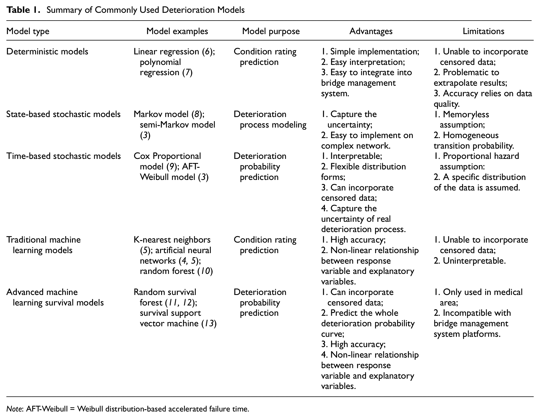
Note: AFT-Weibull = Weibull distribution-based accelerated failure time.

Deterministic models, such as linear regression, polynomial, and logistic regression, are among the more traditional models which are simple to implement and easy to interpret ( 14 ). However, these models do not account for the distribution of the data; they can perform well for the range of the data used but can have significant errors for data outside of the range of data used, for example, predicting negative sojourn times. They also perform well for continuous variables, however, these are rare in the asset management ( 15 ), and they cannot incorporate censored data. On the other hand, stochastic models are more realistic since these models capture the uncertainty of the deterioration process. Based on the model’s purpose, it can be classified as a state-based model or a time-based model. State-based models, such as the Markov chain model ( 8 ) and semi-Markov model ( 3 ), predict the whole deterioration process from the highest condition to the lowest condition and the uncertainty is addressed by a transition probability matrix. However, their performance is limited by the memoryless assumption and homogeneous transition probability ( 16 ). Time-based models focus on predicting the deterioration probability for a given time point, which can be non-parametric and parametric. Generally, non-parametric and semi-parametric models, such as Kaplan-Meier model ( 2 ) and Cox proportional model ( 9 ), can capture the deterioration process more realistically since they are not required to follow a mathematical distribution. However, these models are limited to the range of the available data or may suffer from the proportional hazard assumption. On the other hand, parametric models are simple, efficient, and interpretive. Commonly used distributions for parametric survival models include exponential, Weibull, log-normal, gamma, and generalized gamma distributions (17, 18). Censored and uncensored data are jointly considered in stochastic models by jointly using the hazard function (instantaneous probability of failure) for uncensored data and the reliability function (the cumulative probability of failure) for censored data in the estimation of the models (2, 17). However, the randomness in the deterioration process can lead to these models having low accuracy. Manafpour et al. ( 3 ) developed an AFT-Weibull model to analyze the deterioration process based on the Pennsylvania bridge inspection data, but it takes the traditional sojourn time as the dependent variable, which might underestimate the impact of traffic load on the selection of attributes. Also, the novel machine learning-based approaches might improve the accuracy compared with the AFT-Weibull model used in previous studies.

Machine learning methods have been studied recently for modeling deterioration of the transportation infrastructure ( 19 ). These methods are essentially more intelligent non-parametric models since they rely solely on the data; however, they can learn the trends of the data intelligently to improve the usability of the predictions. One study compared five data mining techniques: logistic regression, decision trees, neural network, gradient boosting, and support vector machine for modeling deterioration of steel bridge superstructure, and found that logistic regression achieved the highest prediction accuracy ( 19 ). Another study showed that the back-propagation neural network can predict bridge deterioration with 75.4% accuracy (10, 20). Assaad and El-Adaway even observed a 91.44% testing accuracy for predicting the condition of a bridge deck using a well-tuned artificial neural network model ( 5 ). Other commonly used machine learning approaches in infrastructure deterioration modeling include k-nearest neighbors, recurrent neural networks, and random forest, in which the ensemble learning algorithms (i.e., random forest) are believed to have superior performance ( 21 ). Even though these machine learning methods have been shown to achieve good prediction accuracy, they only take traditional datasets as input. Therefore, they cannot incorporate censored data nor provide a complete deterioration probability curve for the entire analysis window.

Currently, two advanced machine learning methods that can model survival exist, namely RSF and survival support vector machine (Survival-SVM). RSF is different from the traditional random forest in which the splitting rule for partitioning the dataset and the predicted approach for the terminal leaves are adjusted to incorporate censored data and provide a complete deterioration probability curve. Survival-SVM is an extension of Rank SVM and only treats a pair of ranks as valid when the lower observed time is uncensored since the exact duration of censored data is unknown ( 13 ). Estimating a Survival-SVM can be very complex and time-consuming, especially when the kernel function is complex and the dataset size is large. Thus, RSF is more popular for survival analysis. However, to the authors’ knowledge, these advanced machine learning-based survival models are only used in the medical area. Examples of applications include clinical risk prediction ( 11 ), survival prediction of breast cancer patients ( 12 ), and comparison of survival from different illnesses ( 22 ). Different applications have focused on tailoring the methods to the specific problem considered, such as determining how best to implement the splitting of the tree (11, 12). Further, one study compared the RSF with a Cox regression and demonstrated that the two methods achieved compatible results in modeling breast cancer survival, while RSF showed a slightly better performance than other approaches ( 23 ).

The use of survival machine learning methods in the area of infrastructure deterioration is unknown. Since the infrastructure deterioration and medical survival processes are significantly different in many aspects and possess different deterioration patterns, the appropriate implementation of survival machine learning methods for infrastructure deterioration needs to be studied.

Research Objectives

Based on the literature review, the present study introduces the RSF model into the infrastructure management literature and adapts it for bridge deck deterioration analysis. The performance of RSF is compared with a commonly used traditional stochastic model, that is, the AFT-Weibull model, to analyze the advantages of the different types of modeling approaches. Note that the AFT-Weibull model is chosen as the state-of-the-art model since it has been shown to outperform deterministic models (15, 24, 25) and the Markov model ( 16 ). Weibull distribution is also proved to be the most suitable distribution for infrastructure management compared with exponential, log-normal distribution (15, 26). The purpose of both AFT and RSF models is to predict the deterioration probability for a given time, therefore, they are more comparable than the other models. Based on these advantages, the AFT-Weibull model is selected as a benchmark in this study to shed light on the performance of the RSF model. Further, the RSF method’s independent variable selection process is tailored to the bridge deck deterioration analysis.

The remainder of the paper is organized as follows. The basic theory of RSF and dependent variable selection is introduced in the enxt section, followed by a description of experiments and results. Next, the associated discussions are presented. Finally, key results, limitations, and future research are presented in the concluding section.

Methodology

The major model used in the present study is RSF. In this section, the basic theory of RSF and the major difference from a traditional random forest methodology is outlined.

RSF

RSF is a type of ensemble learning approach that combines a series of basic learners, such as survival trees. The ensemble RSF takes the average of the basic learners’ predictions as the final output, and therefore has higher predictive accuracy and robustness. The basic theory is similar to a traditional random forest. The general construction of a decision tree and a random forest is illustrated in Figure 1. A typical random forest can be described with the following hyperparameters: (a) number of estimators, (b) maximum depth, (c) the minimum number of samples in a leaf, and (d) the maximum number of features considered for splitting. The number of estimators determines the number of trees estimated to be combined for the random forest. As this number increases, the random forest model becomes more robust, but also more complex and difficult to interpret. The maximum depth of the tree determines the number of layers considered. As the tree depth increases, each terminal leaf will be representative of a smaller subset of the data. The minimum number of samples in a leaf is also related to the tree depth, that is, the tree will not be split further once the minimum number of samples in a leaf is met even if the tree depth allows for further splitting. Finally, the maximum number of features considered for splitting represents the number of variables considered in each tree. While all variables are considered for a decision tree, in a random forest method each tree only considers a subset of variables, which improves the robustness of the model and avoids overfitting. Detailed mathematical expressions can be found in the literature ( 27 ).

Figure 1.

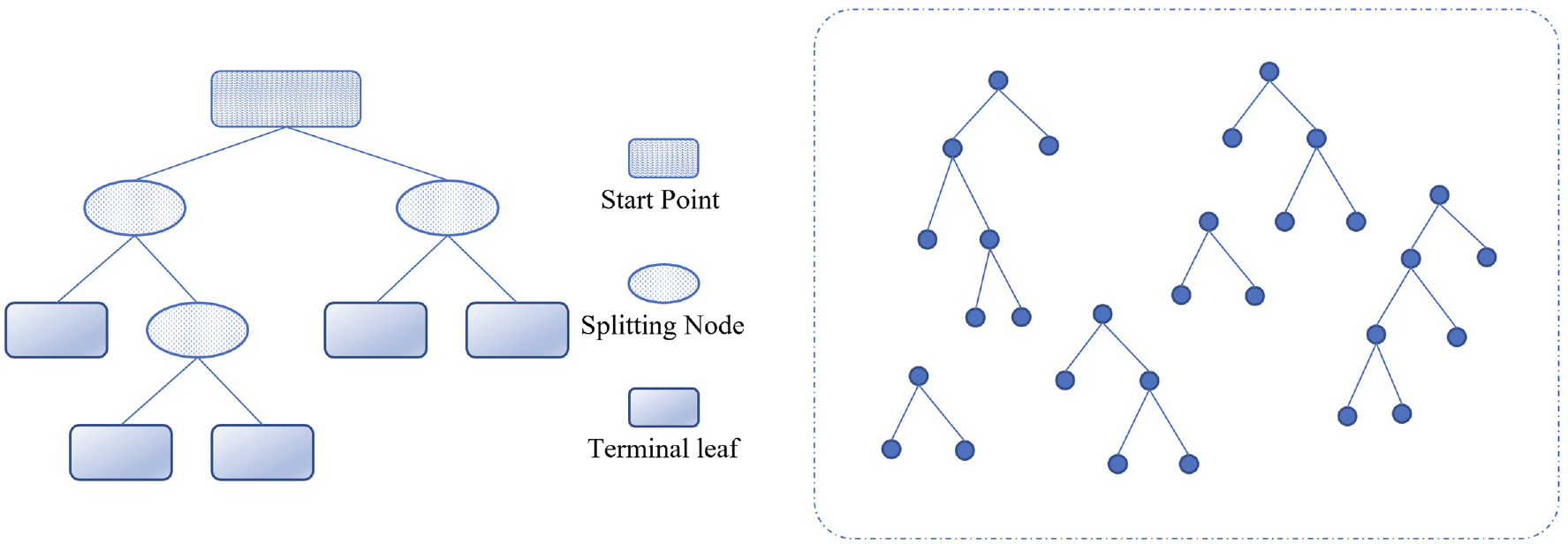
Architecture of a decision tree (left) and a forest (right).

A traditional random forest is a powerful tool, but censored data cannot be incorporated into this model. RSF modifies the traditional random forest to improve the splitting rule, prediction method, and evaluation metric, to be able to account for censored deterioration data. The other approaches used to improve an RSF, like bagging, boosting, and pruning, are similar to the traditional random forest, and thus the details are not repeated here ( 28 ).

Splitting Rule

The splitting rule is used to partition the dataset into subsets that maximize the difference between and minimize the difference within each subset. As a result, observations that share similar characteristics are grouped into the same terminal node, thus a prediction based on the observations within a terminal node can closely represent the data pattern of its members.

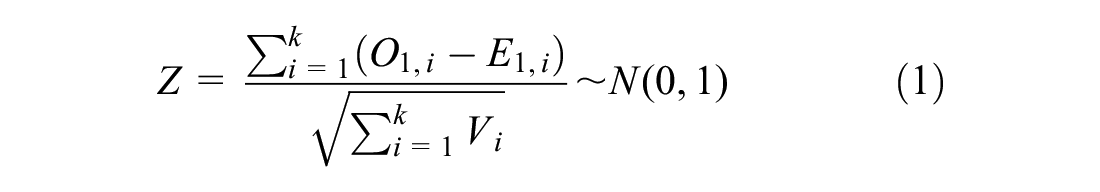
In the traditional random forest, the common splitting rules, such as Gini index and entropy, aim to maximize the similarity of the output within each subset. Normally, the output is a one-dimension variable and has clear equations to measure its similarity. However, for the survival data, the output is two-dimensional, and the final prediction is a complete deterioration probability curve. Thus, the splitting rule in RSF should aim at generating subsets that have the most different deterioration patterns. The log-rank test is commonly used to quantify the difference in the deterioration patterns predicted from each subset ( 29 ). In the log-rank test, the null and alternative hypotheses are:

$H_{0}$ : The deterioration pattern in the two datasets is identical.

$H_{1}$ : The deterioration pattern in the two datasets is significantly different.

The test statistic function for the Z-value to accept the null hypothesis is shown in Equation 1:

Z = \frac{\sum_{i = 1}^{k} (O_{1, i} - E_{1, i})}{\sqrt{\sum_{i = 1}^{k} V_{i}}} ~ N (0, 1)

(1)

where $O_{1, i}$ is the observed number of deaths at the time, $t_{i}$ , in subset 1; $E_{1, i}$ is the expected number of deaths at the time, $t_{i}$ , in subset 1, which can be calculated as $E_{1, i} = \frac{d_{i} Y_{1, i}}{Y_{i}}$ . $Y_{1, i}$ is the number of individuals at risk (neither dead nor censored) at the time $t_{i}$ in subset 1; $d_{i}$ is the number of individuals dead at the time $t_{i}$ .

$V_{i}$ is the variance of the observed number of deaths, which can be calculated as:

V_{i} = \frac{Y_{2, i} Y_{1, i} d_{i} (Y_{i} - d_{i})}{Y_{i}^{2} (Y_{i} - 1)}

(2)

Prediction Method

The prediction method for the RSF relies on the use of a cumulative hazard function (CHF) measured using the Nelson-Aalen estimator. The cumulative hazard represents the aggregated hazard, or instantaneous risk of failure, over time. It can be interpreted as the number of times a failure (i.e., the CR lowering) would be expected over the analysis window. The Nelson-Aalen estimator is much focused on the hazard of the asset during the life cycle. The CHF of the Nelson-Aalen estimator is:

\hat{H} (t) = \sum_{t_{i} < t} \frac{d_{i}}{Y_{i}}

(3)

where $t_{i}$ are the elements of all distinct event times; $d_{i}$ is the number of deaths at the time $t_{i}$ ; and $Y_{i}$ is the total number of individuals at risk (neither dead nor censored) at the time $t_{i}$ .

To predict the Nelson-Aalen estimator for a given terminal leaf, the hazards of all data that fall in that leaf are combined. This can be used to determine the risk of failure at a given time for a new bridge deck.

Evaluation Metric

To understand how well a given RSF performs, the prediction accuracy of that RSF needs to be determined. However, the prediction of the deterioration pattern for a single observation is not necessarily meaningful since the results are probabilistic. Therefore, the performance of the RSF method is evaluated by comparing the ranking of the predicted risk score with the actual survival data in the whole testing dataset. The risk score, $r$ , is the total number of failures expected over the lifetime of the study for a given bridge deck with a set of attributes, $x$ , within the analysis window ( 30 ). This risk score can be estimated as the sum of the estimated CHF, ${\hat{H}}_{h}$ , for a terminal node $h$ as shown in Equation 4.

r = \sum_{j = 1}^{n_{h}} {\hat{H}}_{h} (T_{hj} | x)

(4)

where $n_{h}$ is the number of distinct uncensored times of samples in terminal node $h$ ; $T_{hj}$ is the $j th$ item of these distinct uncensored times in terminal node $h$ .

The model evaluation first predicts the risk scores for a set of bridges in the testing dataset. Next, these bridges are ranked by risk score from lowest to highest. Finally, the ranking of the real (observed) survival times is determined. The ranking from the model prediction is compared with the ranking from the real data. The accuracy of the ranking prediction is measured by the concordance index (C-index), which reflects the ability of a survival model to predict the survival time rank based on the predicted risk scores. The C-index can be computed as Equation 5.

C = \frac{\sum_{i, j} I_{T_{j} < T_{i}}^{*} I_{r_{j} < r_{i}}^{*} δ_{j}}{\sum_{i, j} I_{T_{j} < T_{i}}^{*} δ_{j}}

(5)

where $r_{i}$ is the predicted risk score of a unit $i$ ; $I_{T_{j} < T_{i}} = 1$ if $T_{j} < T_{i}$ else 0; $I_{r_{j} < r_{i}} = 1$ if $r_{j} < r_{i}$ else 0; and $δ_{j}$ denotes the censorship of the data. $δ_{j} = 0$ means uncensored data, $δ_{j} = 1$ means censored data. The range of the C-index is from 0.5 to 1, where $C = 1$ corresponds to the best model prediction, and $C = 0.5$ represents a random prediction.

Finally, the C-index can also be used to measure the importance of different input variables in determining the survival curve. To do so, permutation-based feature importance is calculated by measuring the C-index of the original model and comparing it with the C-index of a shadow model, which is created by randomly shuffling the values of a given attribute in the training data. The difference in the C-index of the original model and shadow model is assumed to be indicative of the importance of that variable in determining the final survival curve. Therefore, the rank of features is determined as the ordered gains in C-index.

Experiments and Results

To demonstrate the performance of RSF in bridge deck deterioration modeling, the dataset of inspection records of 22,000 bridge decks from Pennsylvania is adopted, and a summary of the dataset is described in this section. First, the choice of the dependent variable is explored. Two candidate variables, namely time-in-rating (TIR) and cumulative truck traffic (CTT), are tested. Next, the hyperparameters of the RSF are calibrated, the best structure is demonstrated, and the model is compared with the AFT-Weibull model.

Data Description

The Pennsylvania Department of Transportation conducts regular inspections of approximately 22,000 state-owned bridges at most every two years. In the inspection report, a general condition rating (CR) is assigned to a bridge deck to reflect the general condition of the bridge deck between 1 and 9, where CR 9 represents the best condition. In the present study, the dataset was separated into nine subsets based on the CR. Before developing the model, the dataset is cleaned and processed based on several rules: (a) rows with important data missing are discarded; (b) abnormal data, such as a single outlier CR, are corrected; (c) if the CR changed more than two levels (higher or lower) in between inspections, this change was marked as “sharply increased” or “sharply decreased,” respectively, and recorded in the EVENT variable. These “events” could be reconstruction or incidents that happened to the bridge. After cleaning the raw data, valid information for 18,354 bridges was obtained. The TIR for each CR was extracted, including whether the TIR was censored or not. A TIR with an unobserved startpoint or endpoint, or suffering from an incident or rehabilitation that significantly changed the CR, was treated as a censored data point. A total of 44,086 TIRs were extracted and classified by CR. Summary statistics for the distribution of the TIRs were determined as shown in Table 2.

Table 2.

Statistic of Time-in-Rating Values of Bridge Decks

Condition	Censored			Uncensored
Rating	Count	Mean (days)	Std (days)	Count	Mean (days)	Std (days)
CR 1	19	2,809	2,509	2	1,040	348
CR 2	104	1,690	1,263	13	1,818	1,124
CR 3	1,007	2,022	1,709	170	2,034	1,421
CR 4	3,132	3,197	2,410	783	2,581	1,717
CR 5	6,016	4,010	2,759	2,317	2,935	1,794
CR 6	7,264	4,024	2,622	3,865	2,977	1,719
CR 7	8,636	3,957	2,603	3,817	3,054	1,760
CR 8	3,234	2,610	1,927	2,612	2,501	1,443
CR 9	654	1,420	1,106	381	1,747	1,049
Total	30,066			13,960

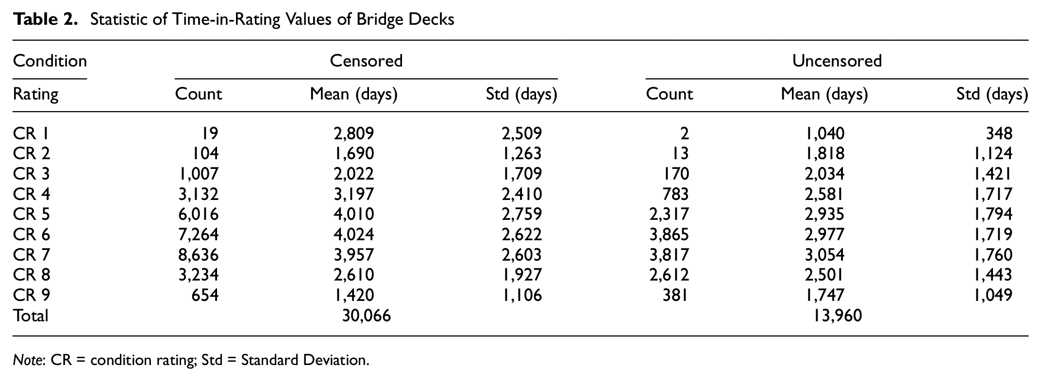
Note: CR = condition rating; Std = Standard Deviation.

It can be seen that only a few bridge decks have uncensored data points with condition ratings lower than CR 4, since typically CR 1 through 3 are considered poor conditions. Thus models of CR 4 and higher are more reliable. In this study, the RSF was illustrated with the sub-dataset of CR 6 and in the following, deterioration probability refers to the probability of a bridge deck deteriorating from CR 6 to CR 5. However, note that similar results were obtained for other CR values.

The attributes of each bridge are the static configuration of the deck structural components, which may accelerate or decelerate the deterioration process. These attributes are incorporated into the model as explanatory variables to analyze their impact on TIR or CTT. The major attributes used in this study are summarized in Table 3.

Table 3.

Description and Values of Attributes, Including the Count of Each Value in the Dataset

Attribute (National Bridge Inventory item number)	Description	Values (counts)
DISTRICT (2)	District number	District 1 (2,707); District 2 (2,102); District 3 (3,171); District 4 (2,200); District 5 (2,215); District 6 (2,912); District 8 (5,369); District 9 (3,497); District 10 (2,443); District 11 (2,672); District 12 (2,817).
BUILT_YEAR (27)	Year of construction	Before 1942 (6,359); 1942–1980 (13,468); after 1980 (5,665)
STRUC_TYP (107)	Deck structure type	Concrete—reinforced (26,324).
MAIN_MATERIAL_TYPE (43A)	Main material types	Steel (8,531); Concrete (cast in place) (6,205); Concrete (precast) (537); Prestressed precast concrete (P/S) (15,774); Concrete encased steel (982).
MAIN_PHYSICAL_TYPE	Physical make-up of the main span of the structure	Reinforced (6,744); Pretensioned (15,600); Rolled sections (4,787); Rolled sections with cover plates (1,174); Combination, rolled sections/cover plates (334); Other (3,313).
MAIN_SPANS (45)	Main bridge spans (number of spans in the main unit.)	Single span (20,209); Multi-span (11,122).
MAIN_STRUC_CONFIG (43)	Structural configuration for the main span of the structure.	Slab (solid) (2,378); T-beams (3,985); I-beams (11,653); Box beam—single (5,681); Box beam—adj (6,614); I-Welded beams (410); Girder weld/deck (722).
DECK_REBAR_TYPE	Deck rebar type.	Bare (12,960); Galvanized (561); Epoxy (11,738); Unknown (6,794).
MEMBTYPE (108B)	Waterproofing membrane on the bridge main span.	None (26,722); Preformed fabric (3,816); Other (368).
SURF_TYPE (108A)	Wearing surface types on the bridge main span.	Concrete overlay (17,543); Epoxy overlay (974); Bituminous (13,340).
LENGTH (112)	Bridge length.	The total overall length of the bridge.
DECK_WIDTH (52)	Bridge deck width.	Bridge deck width.
ADT_Total (29)	Average daily traffic in total	Average daily traffic in total, including all types of vehicles.
ADTT (109)	Average daily truck traffic.	Average daily truck traffic.
SPECIAL EVENT	If a special event happened.	Sharply decrease (3,497); Normal (22,332); Sharply increase (6,212)

Note: Values (counts) only show the values whose count is larger than 1% of the whole dataset.

EVENT is a variable generated during data processing which is used to denote whether rehabilitation or an incident happened to a bridge that sharply increased or decreased the CR of the bridge, respectively. It was determined by checking if the CR changed more than two ratings in a pair of two adjacent inspection points (about 3 years).

Dependent Variable Selection

An appropriate choice of the dependent variable can significantly improve the performance of the model. TIR is a commonly used dependent variable for infrastructure management, which represents the duration for which a bridge has been in a specific condition rating ( 26 ). However, time-based deterioration models may not be able to capture fully the deterioration rate difference of bridge decks since the amount of truck traffic can significantly affect bridge deck deterioration. The annual average daily truck traffic (ADTT) varies across different bridges and influences the design of a bridge deck. ADTT is also a dynamic variable that may change in different years. Based on the TIR and ADTT, the CTT, which reflects the total traffic load that a bridge was exposed to before deteriorating, can be calculated and is monitorable in practice. Therefore, in addition to the TIR, the CTT, calculated as the product of TIR and ADTT in each year, is proposed as an alternative dependent variable. Note that these two variables are independent (e.g., the correlation coefficient is 0.25).

The reliability of a bridge deck denotes the probability of a bridge deck remaining in the same CR for a given time, which equals 1 minus deterioration probability. The reliability analysis for bridge decks using both dependent variables, TIR and CTT, is demonstrated with respect to three typical attributes, that is, rebar type, span number, and surface type, to compare the performance of the two dependent variables.

Rebar Type

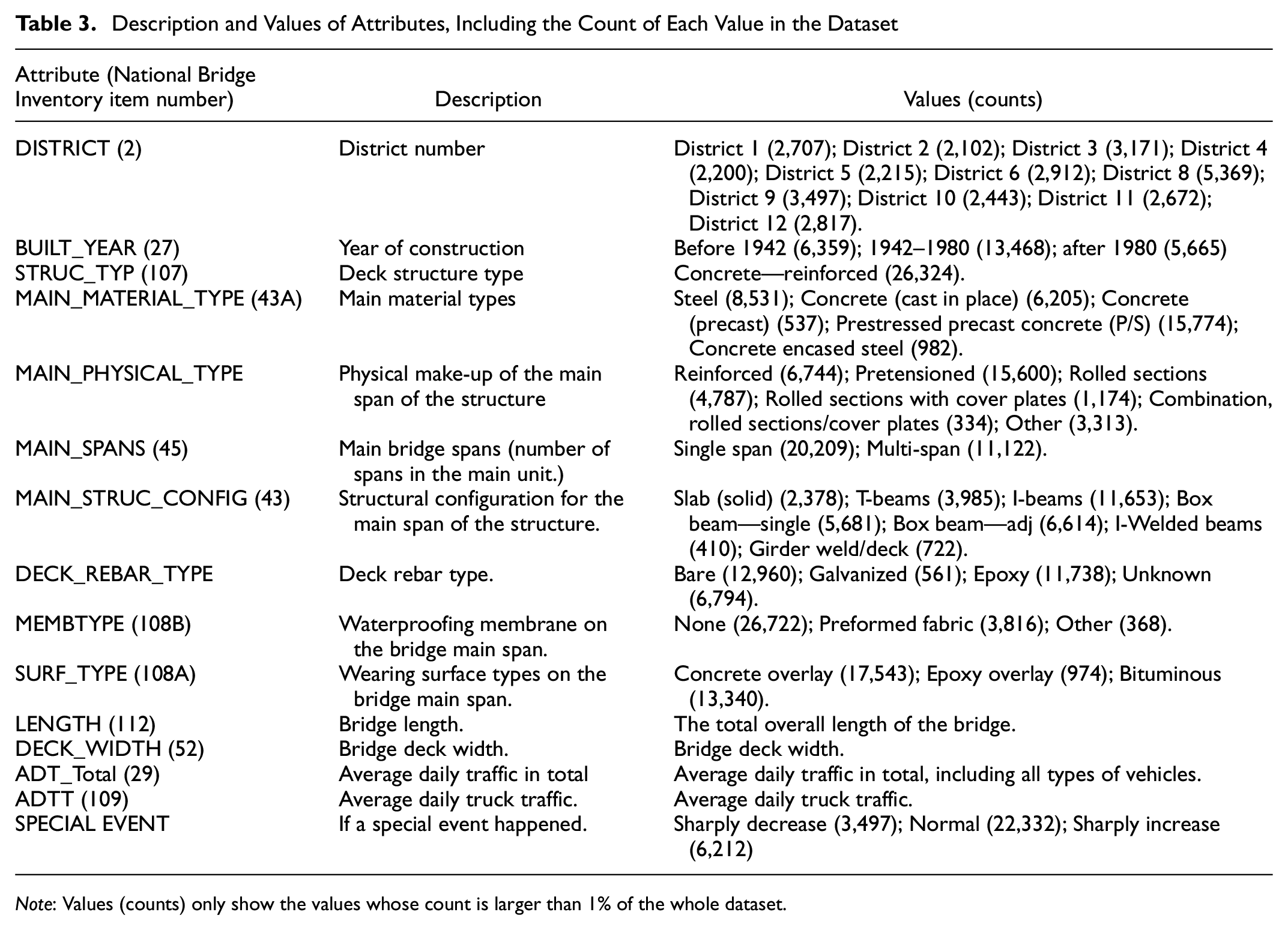
Three different types of rebar used for bridge decks were compared: bare, epoxy-coated, and galvanized. Figure 2a shows the TIR of bridge decks with different CRs and rebar types and suggests that the average TIR (∼7 years) is mostly independent of rebar type. However, the number of the bridges (Figure 2b) and the ADTT that a bridge experienced (Figure 2c) with different rebar types are significantly different. There are more bridges in higher CRs with galvanized or epoxy rebar, and these bridges often experience a higher ADTT. Thus, even though the bridge decks have similar TIRs, the advantage of the galvanized or epoxy rebar might be compromised by the heavier traffic load. Thus, the TIR alone is not enough to reflect the reliability difference of different rebar types. However, the difference in reliability based on rebar type can be seen when considering CTT (Figure 2d). The results suggest that bridge decks with epoxy or galvanized rebar have higher reliability than bare rebar bridges when considering CTT, which aligns with the engineering judgment ( 31 ).

Figure 2.

Distribution for rebar type by condition rating of: (a) time-in-rating, (b) number of bridges, (c) average daily truck traffic, and (d) cumulative truck traffic.

Span Number

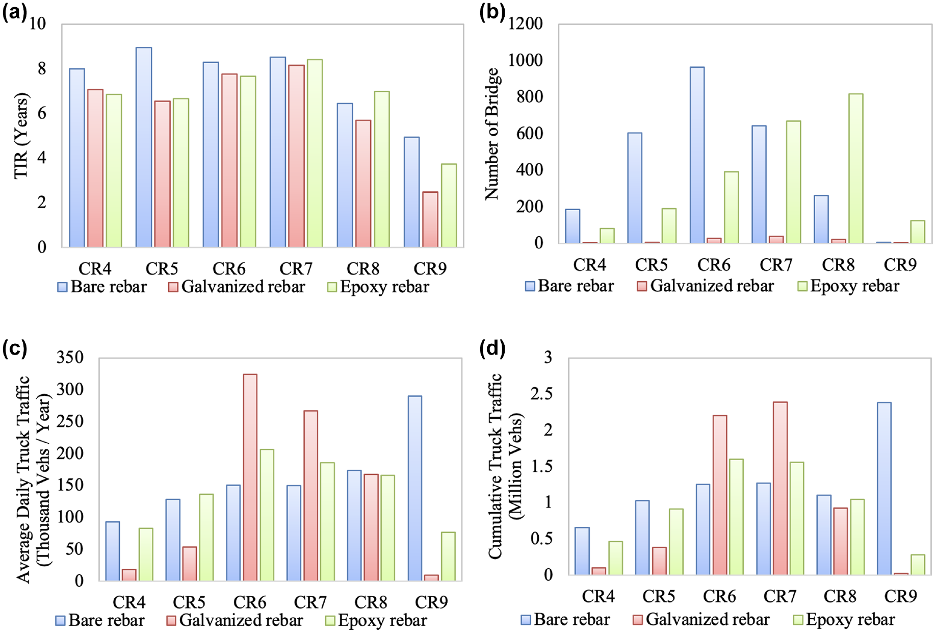
Single-span bridges were compared with multi-span bridges to see trends in deterioration. The average deck length of a single-span bridge is 42 ft, compared with 278 ft for a multi-span bridge. From the TIR distribution, single-span and multi-span bridges perform similarly. However, this does not necessarily indicate that a single-span bridge is as reliable as a multi-span bridge from an engineering perspective. Considering the number of bridges (see Figure 3b) and the ADTT (see Figure 3c), while there are more single-span bridges, the multi-span bridges carry more trucks. This implies that the multi-span bridges are mostly constructed in areas with heavy truck traffic but can still achieve similar TIRs as single-span bridges. This indicates that the multi-span bridges have higher reliability than single-span bridges, which is confirmed by the CTT-based analysis (see Figure 3d).

Figure 3.

Distribution for span type by condition rating of: (a) time-in-rating, (b) number of bridges, (c) average daily truck traffic, and (d) cumulative truck traffic.

Surface Type

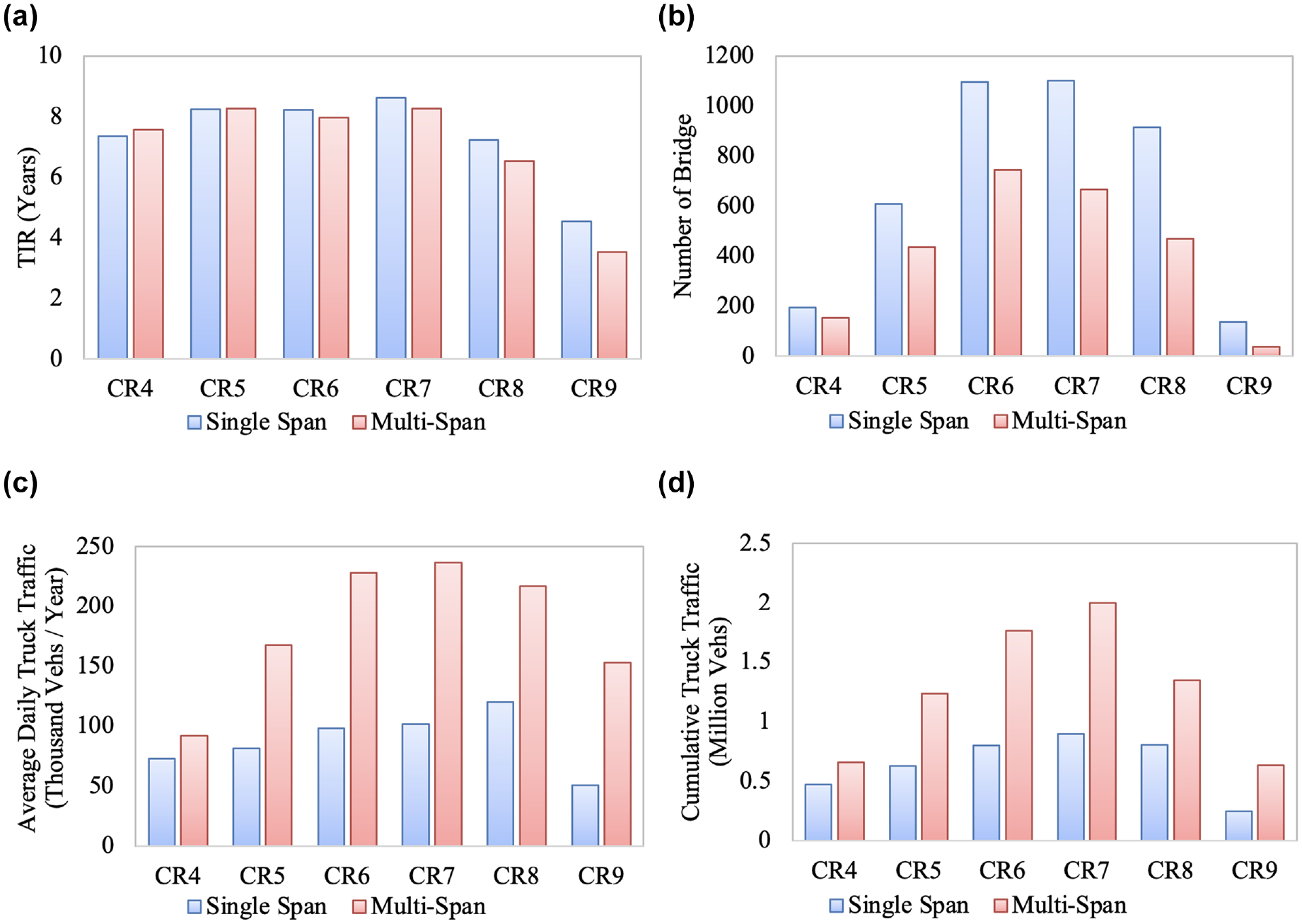
Overlays are used to remedy spalling and cracking for deteriorated bridge surfaces. Comparing the TIRs for the three different overlay materials used (concrete, asphalt, and epoxy) it can be seen that bridge decks that have an asphalt overlay have on average an 8.8% greater TIR, see Figure 4a. However, only a few bridges have an epoxy overlay (see Figure 4b) and these bridges have larger daily truck traffic than bridges with concrete or asphalt overlay (see Figure 4c). Therefore, when considering the CTT, bridges with epoxy overlay have the highest reliability, while bridges with asphalt overlay have the lowest reliability (see Figure 4d). The reliability of the different overlay material considering the CTT is more aligned with field experiments ( 32 ).

Figure 4.

Distribution for surface type by condition rating of: (a) time-in-rating, (b) number of bridges, (c) average daily truck traffic, and (d) cumulative truck traffic.

Overall, comparing the reliability of bridge decks with different rebar types, span numbers, and surface types reveals that CTT can better reflect the reliability of a bridge as compared with TIR and better match engineering judgment. Generally, it might be difficult to capture the reliability difference of the attributes considering only TIR since the design choice is often influenced by expected traffic load.

RSF

In this section, the RSF model is implemented considering TIR and CTT as the dependent variables to further compare their performance. When TIR is the dependent variable, the ADTT is incorporated as one of the covariates, while when CTT is selected as the dependent variable, ADTT is excluded from the model. First, 20% of the data is randomly selected and set aside for testing the trained model performance. The remaining 80% of the data is used to train the model parameters. The model parameters are trained by performing a fourfold cross-validiation, so the remaining training data is divided into four groups. Each group is selected to validate the dataset once, while the remaining groups are used as a training dataset, that is, this process is repeated four times. Therefore, four sets of training-validating datasets are obtained and the average accuracy of these four training and validating datasets is used to select the optimal model specification.

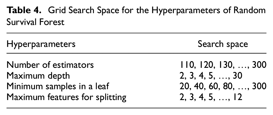
To achieve the best performance of the RSF, the hyperparameters need to be well tuned. The main hyperparameters that need to be tuned include: (a) the number of estimators, (b) maximum depth, (c) minimum samples in a leaf, and (d) the maximum features for splitting. A commonly used approach for tuning the hyperparameters of machine learning methods is grid search, which is also used in the present study ( 5 ). The RSF model is implemented with the Python package scikit-survival ( 30 ). The grid search space for these hyperparameters is shown in Table 4.

Table 4.

Grid Search Space for the Hyperparameters of Random Survival Forest

Hyperparameters	Search space
Number of estimators	110, 120, 130, …, 300
Maximum depth	2, 3, 4, 5, …, 30
Minimum samples in a leaf	20, 40, 60, 80, …, 300
Maximum features for splitting	2, 3, 4, 5, …, 12

The hyperparameters of RSF that achieved the top five performances for the TIR-based model and CTT-based model are shown in Table 5.

Table 5.

Best Model Configuration from Grid Search

Dependent variable	Rank	Number of estimators	Max. depth	Min. samples in a leaf	Max. no. of features for splitting	Average C-index on training datasets	Average C-index on validating datasets	C-index on testing dataset
Time-in-rating	1	200	12	20	5	0.7382	0.6088	0.5913
	2	200	12	40	5	0.6874	0.6060	0.5937
	3	200	12	60	5	0.6619	0.5973	0.5901
	4	200	12	80	5	0.6464	0.5929	0.5876
	5	220	12	200	10	0.6115	0.5869	0.5891
Cumulative truck traffic	1	270	18	200	8	0.8562	0.8476	0.8362
	2	100	18	200	8	0.8553	0.8476	0.8360
	3	200	18	200	8	0.8550	0.8475	0.8352
	4	200	16	200	8	0.8550	0.8475	0.8353
	5	200	13	200	8	0.8560	0.8472	0.8356

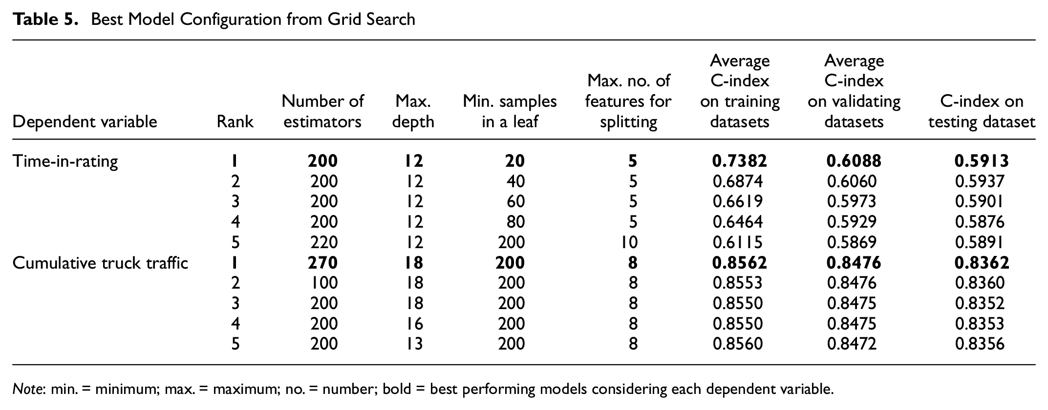
Note: min. = minimum; max. = maximum; no. = number; bold = best performing models considering each dependent variable.

The results suggest that the CTT-based models outperformed the TIR-based model in predictive score in both validation and testing datasets. The CTT model was able to obtain 83.62% accuracy on the testing dataset compared with the TIR model at 59.13% when measured by C-index. This further confirms that the dependent variable of CTT can provide better differentiation for the impacts of the attributes on deterioration.

The best CTT-based model consisted of 270 estimators. As the number of estimators increase, the advantage of the ensemble approach becomes apparent and the accuracy of the model increases. However, increasing the number of estimators beyond 270 no longer improves the accuracy, but increases the complexity of the model. The optimal maximum depth is found to be 18, and the minimum number of samples in a leaf is found to be 200. These two hyperparameters together determine the size of each tree. When the tree is deep, the number of samples in a leaf became small, and the deterioration curve based on these samples becomes too specific and not representative of general categories. When the tree is too small, the dataset is not partitioned enough, and the information available from the covariates is not fully explored. The maximum number of features for splitting can help control the amount of randomness of the RSF. The optimal value of this is eight, which denotes that in each splitting node, the model randomly selects eight out of the total of 12 features used in this study (as shown in Table 3) to search for the best splitting point. This helps build a diverse set of decision trees for the random forest and helps avoid overfitting.

With the well-tuned RSF model, the deterioration curve for a new observation can be predicted. The importance rank of each feature in the RSF determined as a result of the permutation-based feature importance is shown in Figure 5.

Figure 5.

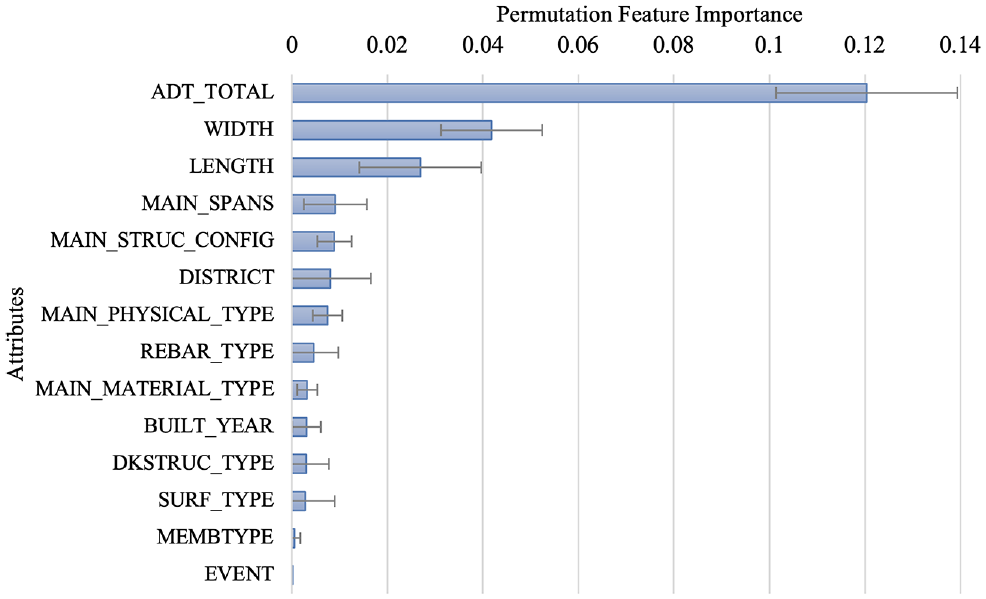
Permutation-based feature importance.

From the feature importance results, it can be found that the traffic load and the size of a bridge, including the width, length, and the number of spans in the main units, are the factors most influential to the deterioration process. This is consistent with the conclusions of research for Indiana’s bridge deterioration analysis from Moomen et al. ( 14 ). Other than this, Moomen also concluded that the environmental (climate) variables, such as freeze index in 1,000s of degree-days, or the average annual number of freeze-thaw cycles, are also critical to the deterioration rate, which are unfortunately not available for the present study. However, the district variable not only represents the maintenance policies that are very different among different locations but also processes geographical diversity (both terrain and weather). It can be seen as a surrogate to the climate variables, and is ranked high from the RSF model. Another deterioration model for Indiana bridges ( 24 ) found that REGION is not statistically significant when predicting TIR, since the climate variables are included as independent variables. The surface type and membrane type were ranked lower by the model. This could be the result of the correlation between the wearing surface system and the other attributes, such as traffic load, district, and bridge size.

To further illustrate the deterioration curve of individual bridges with different attribute values, the DISTRICT attribute is selected for illustration. The survival function for five new bridges, all assumed to be in different districts but with the same attributes, is constructed and are shown in Figure 6. This figure illustrates the survival probabilities at CR 6 obtained by averaging the survival curves from all the trees in the terminal nodes of the RSF. As can be seen, the RSF model can differentiate the survival probabilities of bridges with different attributes. The bridges from districts 2 and 4, which are near Philadelphia, have higher survival probabilities than bridges from other districts when all the other attributes remain the same. This is consistent with the expectation that the districts near big cities have larger budgets, therefore, the bridge decks in those areas are stronger than other places. On the other hand, this curve also provides a life expectation in respect of CTT rather than time, such as done by Srikanth and Arockiasamy ( 15 ). For example, the curves shown in Figure 6 represent the probability of deterioration from CR 6 to CR 5. When the CTT is up to 2 million trucks, the survival probability decreased to around 30%. If we assume a survival probability lower than 30% is unacceptable and denotes the end of the current CR, based on the ADTT, the expected life span in CR 6 can be calculated. For example, the average ADTT in the dataset is 955 trucks/day, then the average lifespan of the bridge shown in Figure 6 can be calculated as 5.7 years. This is roughly consistent with the summary in Srikanth and Arockiasamy ( 15 ) that reinforced bridge decks survive between 24 to 48 years if the threshold of CR 4 is applied as the minimum acceptable CR. However, since the ADTT varies dramatically in the dataset, the specific expected life span of each bridge can be different as well.

Figure 6.

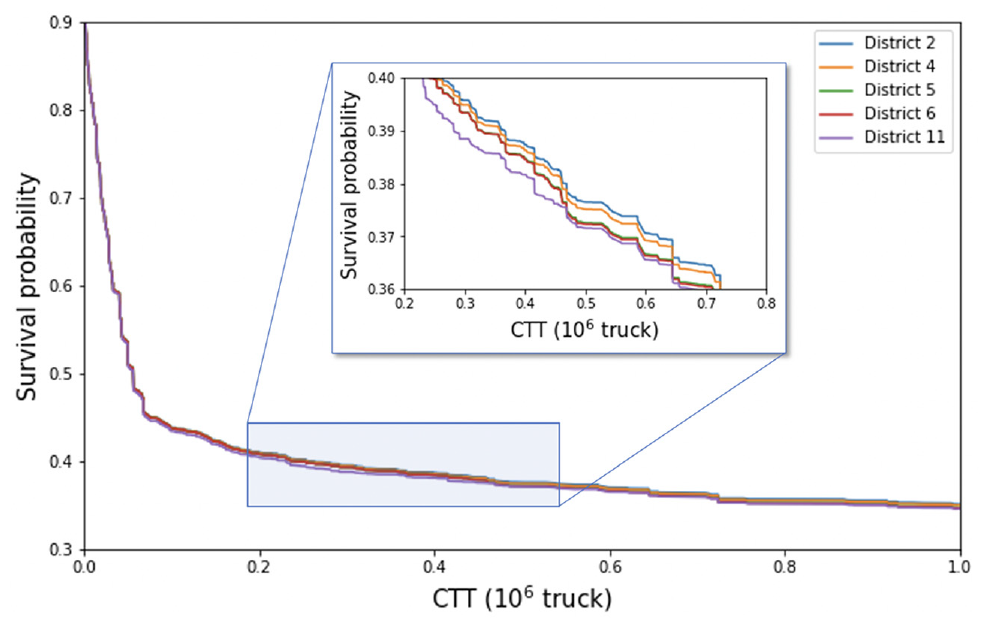
Survival function predictions of bridge decks from different districts while other attributes remain the same.

Comparison with AFT-Weibull Model

To compare RSF with traditional deterioration models, a Weibull distribution-based accelerated failure time model is chosen as a benchmark, which is commonly used in the infrastructure deterioration analysis (3, 33). The AFT-Weibull model can take any bathtub shape distribution as the basic deterioration function and, therefore, is proved to be more appropriate than other distribution-based models.

The probability density function (PDF) of the AFT-Weibull distribution, $f (t)$ , is shown in Equation 6.

f (t, X, β, k) = {\begin{matrix} \frac{k}{e^{β X}} {(\frac{t}{e^{β X}})}^{k - 1} e^{- {(\frac{t}{e^{β X}})}^{k}} & t \geq 0 \\ 0 & t < 0 \end{matrix}

(6)

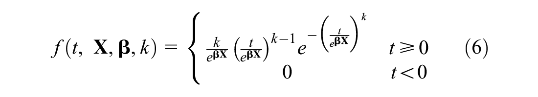
where $t$ is the dependent variable, in this case, CTT; $β$ and $k$ are the parameters of the AFT-Weibull distribution, and $X$ is the vector of covariates. $e^{β X}$ is the accelerated failure term to incorporate the covariates.

The probability of a bridge deck deteriorating to a lower CR can be modeled by the cumulative density function (CDF). The equation for the CDF of the Weibull distribution, $F (t)$ , is shown as Equation 7.

F (t) = 1 - e^{- {(\frac{t}{e^{β X}})}^{k}}

(7)

The AFT-Weibull model is implemented on the same bridge deck deterioration data with CTT as the dependent variable. Here, 80% of the data is used to estimate the model and the remaining 20% of the data is used to test the model performance. Both censored data and uncensored data are incorporated by the PDF and CDF, respectively, in the likelihood function ( 33 ). The model is estimated with a Python package lifeline ( 34 ), and the parameters are estimated using the maximum likelihood estimation approach. The model is well tuned to achieve the highest accuracy, and the parameters are estimated using the maximum likelihood estimation approach as shown in Table 6. Table 6 shows the coefficient of each variable, along with the corresponding p-value, which denotes the confidence level. Note that in the AFT-Weibull model a positive coefficient implies longer survival times. When categorical variables are considered, the coefficients should be interpreted as compared with the baseline, for example, reinforced concrete structure type has a positive coefficient which leads to longer survival times compared with other types of structures. The results suggest that the district, rebar type, deck width, and total ADT are significant variables in predicting bridge deck deterioration probability. The district variable shows a significant influence on the reliability of bridges since it not only represents the maintenance policies that vary among different locations but also has geographic diversity (both terrain and weather). The signs of these coefficients are consistent with engineering judgment. For example, the baseline of the wearing surface type is selected as epoxy overlay and low-slump concrete, and the sign of the coefficients of concrete, concrete overlay, and asphalt are all negative, which implies that epoxy overlay and low-slump concrete are the strongest surface. This is consistent with engineering judgment and the results shown in Figure 4. Bridges that were built between 1943 and 1980 appear to be stronger than the bridges built before 1940 or after 1980 because of the positive coefficient of this variable. This is expected since the data indicates that bridges constructed between 1940 and 1980 generally carry more load. The member type, which are less important variables in the RSF model, were found to be insignificant in the AFT-Weibull model as well. Surprisingly, length, which was ranked third in the RSF model, was not found to be significant in the AFT-Weibull model.

Table 6.

AFT-Weibull Model Coefficient Estimations

Attribute	Value	Coefficient	P-value
DISTRICT	5	−0.21	0.07
	6	−0.93	<0.005
	9	−0.92	<0.005
	11	−0.87	<0.005
STRUC_TYP	Concrete reinforced	0.4	0.06
MAIN_MATERIAL_TYPE	Prestressed precast concrete	−0.66	0.04
MAIN_PHYSICAL_TYPE	Pretensioned	0.51	0.1
MAIN_PHYSICAL_TYPE	Rolled sections	−0.3	0.02
MAIN_SPANS		0.04	0.07
REBAR_TYPE	Epoxy rebar	0.17	0.09
REBAR_TYPE	Galvanized rebar	0.26	0.02
SURF_TYPE	Concrete	−0.74	<0.005
	Concrete overlay	−0.58	<0.005
	Asphalt	−0.49	<0.005
BUILT_YEAR	1943–1980	0.4	<0.005
WIDTH		0.01	0.08
ADT_TOTAL		5.20E-05	<0.005
Intercept		4.06	<0.005
k		0.21	<0.005

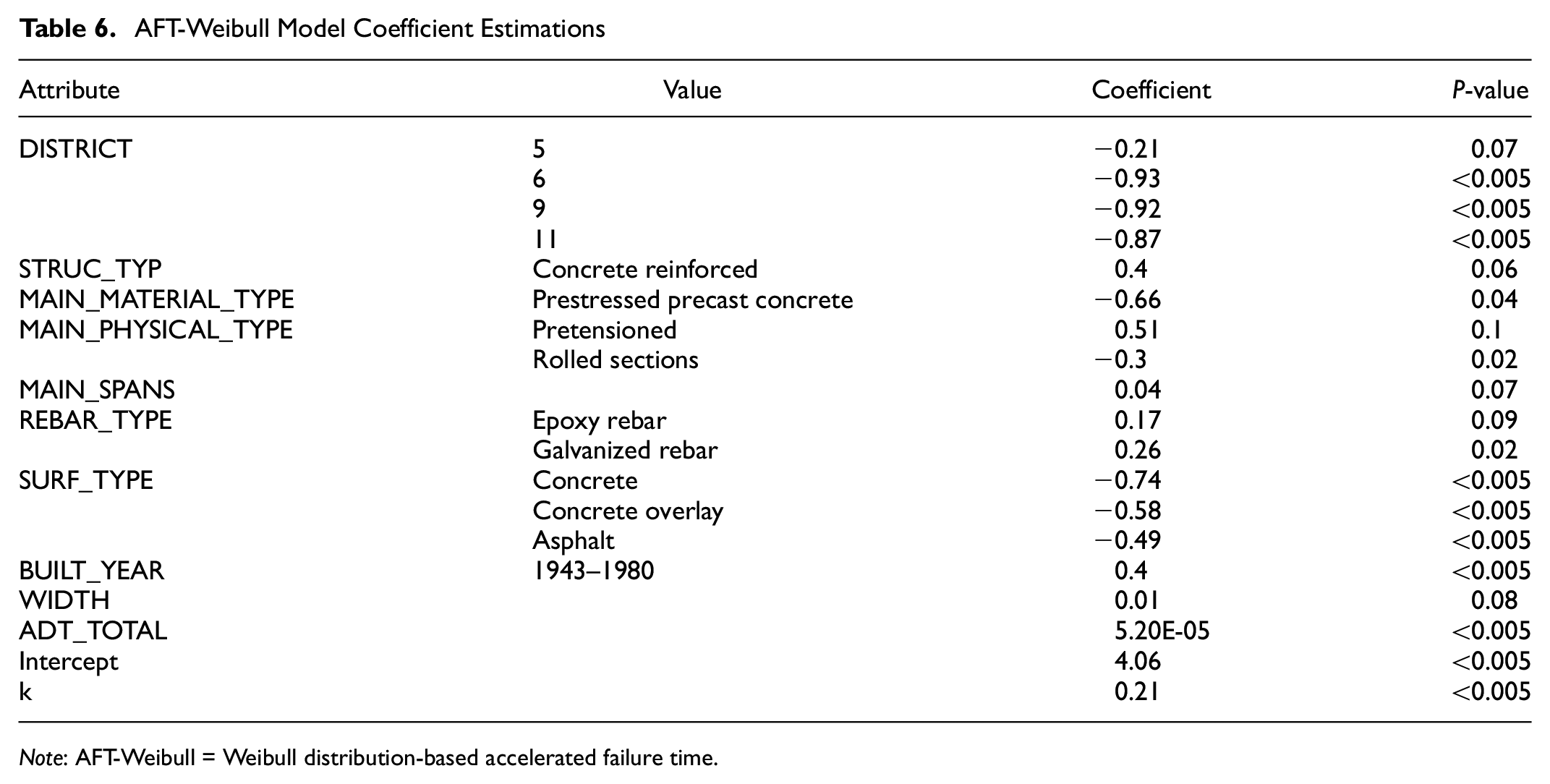
Note: AFT-Weibull = Weibull distribution-based accelerated failure time.

The log-likelihood, which describes the joint probability of the observed data as a function of the parameters of the estimated model, on the training dataset is −343.31. To make a uniform standard to compare the performance of the RSF and AFT-Weibull models, the C-index is used as an indicator of the model’s prediction accuracy, see Equation 5. The attributes and CTT of bridge decks in the same testing dataset are input into the RSF and AFT-Weibull models to calculate the corresponding deterioration probabilities. The ranking of those deterioration probabilities is compared with the real CTT and the associated censorships, and the accuracy of deterioration probabilities is measured by C-index. Therefore, a higher C-index represents a better model performance. The C-index of the AFT-Weibull model in the training dataset is 73.74%, and the C-index for the predictions of the testing dataset is 69.31%. The accuracy of the AFT-Weibull model on the testing dataset is much lower than the accuracy of the RSF model at 83.62%. Since the AFT-Weibull model is proved to be more accurate than other stochastic models (15, 25, 26), these results might indicate that the RSF is more powerful than traditional stochastic models for predicting infrastructure deterioration.

Discussion

TIR versus CTT

The present study showed that CTT is more suitable to be the dependent variable of bridge deck deterioration models than TIR, which is commonly used in survival analysis. From a practical perspective, this is because the influence of TIR on reliability is compromised by the selection of attribute values in the bridge design process. Engineers tend to select stronger materials or structures for bridges that are expected to experience heavier traffic, which leads to all bridges, regardless of the type of construction or materials, having a similar lifespan. Thus, it is difficult to distinguish reliability from a temporal perspective. However, the CTT reflects the actual traffic load that a bridge experiences, which is the main contributor to deterioration (along with the environment), and thus can differentiate the reliability of a bridge more accurately. It is also feasible to use a CTT-based model for a real infrastructure management process, since the traffic load of a bridge is usually closely monitored, and the data is easily collected during regular inspection.

RSF versus AFT-Weibull

This paper indicates that RSF has higher predictive accuracy than the AFT-Weibull model measured by C-index. RSF also can provide the importance of each feature, shown in Figure 5, which is helpful to determine the components critical to design and maintenance of a bridge deck. The AFT-Weibull model, on the other hand, is more suitable to analyze the impact on the reliability of different attribute values, since the coefficient for each attribute value is estimated. Take the coefficient estimations for the rebar type variable in Table 6 as an example. The coefficient estimation for bare rebar is 0.17, and the coefficient for galvanized rebar is 0.26. Both coefficients have low p-values, 0.09 and 0.02, respectively, which denote high confidence levels. Further, variables with larger coefficients represent a longer lifespan, so galvanized rebar is found to be statistically more reliable than the bare rebar, which confirms the results found from the analysis of the raw data. In respect of the model specification, the interpretation of the impact of attribute values in RSF is not intuitive, while the AFT-Weibull model is a typical parametric method, which is simpler and can be explicitly formulated. This can help the integration of the deterioration model with a bridge management system platform, such as AASHTOWare Bridge Management System.

Overall, even though RSF outperformed the AFT-Weibull model in prediction accuracy, the model selection should be based on the research purpose, data quality, and application scenario.

Engineering Significance

From an engineering perspective, the RSF model introduced in this study improved the prediction accuracy of the deterioration probability for a bridge deck and, therefore, can aid in the decision process of maintenance, repair, and reconstruction to improve budget allocation. For a newly constructed bridge, the initial deterioration curve can be predicted by inputting the key attributes of the bridge into the RSF model and the maximum acceptable period for a bridge deck to remain at the same CR can be derived based on pre-defined thresholds of reliability. Further, the RSF model can be used to design bridge decks that can survive longer when considering different attributes.

The RSF model also can be integrated with other life-cycle deterioration analysis models, such as providing the transition probability matrix for the Markov chain model. By acquiring the deterioration probability of each CR from the RSF model, the entire deterioration process of the bridge in its life cycle can be predicted.

Conclusion

This paper introduced the RSF (typically used in the medical field) into infrastructure deterioration analysis, adapted it to bridge deck deterioration modeling, and compared its results with a state-of-the-art AFT-Weibull model. CTT is chosen as the dependent variable, over TIR since experiment results suggest that CTT reflects the reliability of a bridge more accurately. The adapted RSF achieved a much higher predictive accuracy in the testing dataset when considering CTT as the dependent variable, 83.62% (C-index), as compared with 59.13% for TIR as the dependent variable. Further, the RSF model with CTT as the dependent variable also outperformed a representative stochastic model, the AFT-Weibull model that also uses the CTT as the dependent variable (69.31%). The results suggest that RSF has advantages in predicting the rank of risks of bridge decks, providing a complete deterioration probability curve, and determining the feature importance. The RSF model’s use scenarios are different from stochastic models since the RSF is a non-parametric method with higher predictive ability but lower interpretability of the impact of attribute values.

Different enhancements of RSF should be considered for future studies, such as alternative splitting rules, boosting, bagging, and pruning techniques that are commonly used in the traditional random forest. Bridge length multiplied by the ADTT reflects the exposure of a bridge to the truck traffic, and this could be another possible dependent variable candidate for the deterioration model. This can be further tested for future study.

Footnotes

Acknowledgements

The authors gratefully acknowledge the Pennsylvania Department of Transportation for making the data available.

Author Contributions

The authors confirm contribution to the paper as follows: study conception and design: M. Lu, S. I. Guler; data collection: M. Lu, S. I. Guler; analysis and interpretation of results: M. Lu, S. I. Guler; draft manuscript preparation: M. Lu. All authors reviewed the results and approved the final version of the manuscript.

Declaration of Conflicting Interests

The author(s) declared no potential conflicts of interest with respect to the research, authorship, and/or publication of this article.

Funding

The author(s) disclosed receipt of the following financial support for the research, authorship, and/or publication of this article: This work was supported by funds available through the Center for Integrated Asset Management for Multi-modal Transportation Infrastructure Systems (CIAMTIS): Region 3 University Transportation Center, Project number: CIAM-UTC-REG21.

ORCID iDs

Muyang Lu

S. Ilgin Guler

Data Accesibility Statement

The data that support the findings of this study are available from the Pennsylvania Department of Transportation (PennDOT). Restrictions apply to the availability of these data, which were used under license for this study. Data are available from the authors with the permission of PennDOT.

References

Lunn

McNeil

Applying Cox Regression to Competing Risks. Biometrics, Vol. 51, No. 2, 1995, pp. 524–532.

Goyal

Whelan

M. J.

Cavalline

T. L.

Multivariable Proportional Hazards-Based Probabilistic Model for Bridge Deterioration Forecasting. Journal of Infrastructure Systems, Vol. 26, No. 2, 2019, p. 04020007. https://doi.org/10.1061/(ASCE)IS.1943-555X.0000534.

Manafpour

Guler

Radlińska

Rajabipour

Warn

Stochastic Analysis and Time-Based Modeling of Concrete Bridge Deck Deterioration. Journal of Bridge Engineering, Vol. 23, No. 9, 2018, p. 04018066. https://doi.org/10.1061/(ASCE)BE.1943-5592.0001285.

Fathi

Mazari

Saghafi

Hosseini

Kumar

Parametric Study of Pavement Deterioration Using Machine Learning Algorithms. In Airfield and Highway Pavements 2019: Innovation and Sustainability in Highway and Airfield Pavement Technology ( Al-Qadi

Ozer

Loizos

Murrell

, eds.), American Society of Civil Engineers, Reston, VA, 2019, pp. 31–41. https://doi.org/10.1061/9780784482476.004.

Assaad

El-Adaway

I. H.

Bridge Infrastructure Asset Management System: Comparative Computational Machine Learning Approach for Evaluating and Predicting Deck Deterioration Conditions. Journal of Infrastructure Systems, Vol. 26, No. 3, 2020, p. 04020032. https://doi.org/10.1061/(ASCE)IS.1943-555X.0000572.

Zhang

Durango-Cohen

P. L.

Explaining Heterogeneity in Pavement Deterioration: Clusterwise Linear Regression Model. Journal of Infrastructure Systems, Vol. 20, No. 2, 2014, p. 04014005. https://doi.org/10.1061/(ASCE)IS.1943-555X.0000182.

Bolukbasi

Mohammadi

Arditi

Estimating the Future Condition of Highway Bridge Components Using National Bridge Inventory Data. Practice Periodical on Structural Design and Construction, Vol. 9, No. 1, 2004, pp. 16–25. https://doi.org/10.1061/(ASCE)1084-0680(2004)9:1(16).

Semaan

Dib

Comparison Between the Predicted Performance Curve and the Markov Chain Models for Structural Performance of Infrastructure Components. MATEC Web of Conferences, Vol. 289, 2019, p. 08006. https://doi.org/10.1051/matecconf/201928908006.

Mauch

Madanat

Semiparametric Hazard Rate Models of Reinforced Concrete Bridge Deck Deterioration. Journal of Infrastructure Systems, Vol. 7, No. 2, 2001, pp. 49–57. https://doi.org/10.1061/(ASCE)1076-0342(2001)7:2(49).

10.

Bashar

M. Z.

Torres-Machi

Performance of Machine Learning Algorithms in Predicting the Pavement International Roughness Index. Transportation Research Record: Journal of the Transportation Research Board, 2021. 2675: 226–237.

11.

Schmid

Wright

Ziegler

On the Use of Harrell’s C for Clinical Risk Prediction via Random Survival Forests. arXiv Preprint arXiv:1507.03092 [stat], 2016.

12.

Wright

M. N.

Dankowski

Ziegler

Unbiased Split Variable Selection for Random Survival Forests Using Maximally Selected Rank Statistics. Statistics in Medicine, Vol. 36, No. 8, 2017, pp. 1272–1284. https://doi.org/10.1002/sim.7212.

13.

Belle

V. V.

Pelckmans

Suykens

J. A. K.

Huffel

S. V.

Survival SVM: A Practical Scalable Algorithm. In Proc., Advances in Computational Intelligence and Learning: ESANN-European Symposium on Artificial Neural Networks, Bruges, Belgium, April 23–25, 2008.

14.

Moomen

Qiao

Agbelie

Labi

Sinha

Bridge Deterioration Models to Support Indiana’s Bridge Management System. JTRP Technical Reports. Purdue University, West Lafayette, IN, 2016. https://doi.org/10.5703/1288284316348.

15.

Srikanth

Arockiasamy

Deterioration Models for Prediction of Remaining Useful Life of Timber and Concrete Bridges: A Review. Journal of Traffic and Transportation Engineering (English Edition), Vol. 7, No. 2, 2020, pp. 152–173. https://doi.org/10.1016/j.jtte.2019.09.005.

16.

Thompson

P. D.

Ford

K. M.

Estimating Life Expectancies of Highway Assets. National Research Council (U.S.), National Cooperative Highway Research Program, American Association of State Highway and Transportation Officials, Transportation Research Board, Washington, D.C., 2012.

17.

de Pascoa

M. A. R.

Ortega

E. M. M.

Cordeiro

G. M.

The Kumaraswamy Generalized Gamma Distribution with Application in Survival Analysis. Statistical Methodology, Vol. 8, No. 5, 2011, pp. 411–433. https://doi.org/10.1016/j.stamet.2011.04.001.

18.

Edirisinghe

Setunge

Zhang

Application of Gamma Process for Building Deterioration Prediction. Journal of Performance of Constructed Facilities, Vol. 27, No. 6, 2013, pp. 763–773. https://doi.org/10.1061/(ASCE)CF.1943-5509.0000358.

19.

Contreras-Nieto

Shan

Lewis

Characterization of Steel Bridge Superstructure Deterioration Through Data Mining Techniques. Journal of Performance of Constructed Facilities, Vol. 32, No. 5, 2018, p. 04018062. https://doi.org/10.1061/(ASCE)CF.1943-5509.0001205.

20.

Huang

Y.-H.

Artificial Neural Network Model of Bridge Deterioration. Journal of Performance of Constructed Facilities, Vol. 24, No. 6, 2010, pp. 597–602. https://doi.org/10.1061/(ASCE)CF.1943-5509.0000124.

21.

Piryonesi

S. M.

El-Diraby

A Machine-Learning Solution for Quantifying the Impact of Climate Change on Roads. Proc., CSCE Annual Conference, Canadian Society for Civil Engineering, Laval, Quebec, Canada, 2019.

22.

Nasejje

J. B.

Mwambi

Dheda

Lesosky

A Comparison of the Conditional Inference Survival Forest Model to Random Survival Forests Based on a Simulation Study as Well as on Two Applications with Time-to-Event Data. BMC Medical Research Methodology, Vol. 17, No. 1, 2017, p. 115. https://doi.org/10.1186/s12874-017-0383-8.

23.

Omurlu

I. K.

Ture

Tokatli

The Comparisons of Random Survival Forests and Cox Regression Analysis with Simulation and an Application Related to Breast Cancer. Expert Systems With Applications, Vol. 36, No. 4, 2009, pp. 8582–8588. https://doi.org/10.1016/j.eswa.2008.10.023.

24.

Christofas

P. M.

Karlaftis

M. G.

Bridge Deck Deterioration: A Parametric Hazard-Based Duration Modeling Approach. In Advances in Bridge Maintenance, Safety Management, and Life-Cycle Performance, book & CD-ROM ( da Sousa Cruz

P. J.

Frangopol

D. M.

Canhoto Neves

L. C.

, eds.), CRC Press, London, 2015.

25.

Chang

Maguire

Condition Rating Prediction Using an Interactive Deterioration Model Development Package. Applied Sciences, Vol. 10, No. 24, 2020, p. 8946. https://doi.org/10.3390/app10248946.

26.

Sobanjo

J. O.

State Transition Probabilities in Bridge Deterioration Based on Weibull Sojourn Times. Structure and Infrastructure Engineering, Vol. 7, No. 10, 2011, pp. 747–764. https://doi.org/10.1080/15732470902917028.

27.

Biau

Scornet

A Random Forest Guided Tour. Test, Vol. 25, No. 2, 2016, pp. 197–227. https://doi.org/10.1007/s11749-016-0481-7.

28.

Ishwaran

Kogalur

U. B.

Blackstone

E. H.

Lauer

M. S.

Random Survival Forests. The Annals of Applied Statistics, Vol. 2, No. 3, 2008, pp. 841–860. https://doi.org/10.1214/08-AOAS169.

29.

Wellek

A Log-Rank Test for Equivalence of Two Survivor Functions. Biometrics, Vol. 49, No. 3, 1993, pp. 877–881. https://doi.org/10.2307/2532208.

30.

Pölsterl

Scikit-Survival: A Library for Time-to-Event Analysis Built on Top of Scikit-Learn. Journal of Machine Learning Research, Vol. 21, No. 212, 2020, pp. 1–6.

31.

Yeomans

S. R.

Applications of Galvanized Rebar in Reinforced Concrete Structures. Presented at the CORROSION 2001, Houston, TX, 2001.

32.

Sprinkel

Maintenance of Concrete Bridges. Transportation Research Record: Journal of the Transportation Research Board, 2001. 1749: 60–63.

33.

Ashraf-Ul-Alam

Khan

A. A.

Generalized Topp-Leone-Weibull AFT Modelling: A Bayesian Analysis with MCMC Tools Using R and Stan. Austrian Journal of Statistics, Vol. 50, No. 5, 2021, pp. 52–76.

34.

Davidson-Pilon

Lifelines: Survival Analysis in Python. Journal of Open Source Software, Vol. 4, No. 40, 2019, p. 1317.