Capacity Gains of Splitting Cross-Traffic into Multiple Sub-Streams

Abstract

Traffic flow might be limited by cross-traffic which has priority. A typical example of such a situation is a location where cyclists or pedestrians cross a stream of car traffic. Splitting the cross-traffic into two separate sub-streams (for instance left–right and right–left) can increase the capacity of the main stream. This is because it is no longer necessary to have a sufficiently large gap in both sub-streams simultaneously. This paper introduces a method to compute the resulting capacity of roads with cross-traffic. Without loss of generality, we introduce three transformations to simplify computations. These transformations are an important contribution of the paper, allowing us to create scalable graphs for capacity. Overall, the research shows that splitting a crossing stream into two equally large sub-streams increases the capacity of the main stream. If there is place for one vehicle in between two sub-streams, the capacity can increase up to threefold. Even larger gains are possible with more vehicles in between. This paper presents graphs which can be used to find the capacity for generic situations, and can be used for developing guidelines on intersection design.

Urban environments face traffic congestion. For this and other reasons, the use of cycling or walking as mode of transport is promoted. There are various ways to do so, one of which is prioritizing cyclist traffic at unsignalized intersections or crossings. Currently, at the best of the authors’ knowledge, no tools are readily available to assess whether additional measures are needed to improve vehicular traffic flow in this situation; Dutch handbooks ( 1 ) lack such information. This lack of tools is currently becoming more important because of the increase in cyclist traffic, which will also affect the circulation of vehicular traffic.

If vehicles have to share the road with cyclists, the traffic performance for cars is reduced. Cars have to slow down for slower traffic (i.e., cyclists), thus reducing the overall speed for cars. This has been mathematically elaborated in Yuan et al. ( 2 ). Also macroscopic traffic models have been developed for traffic flow with multiple classes. For an overview of macroscopic models, see van Wageningen-Kessels et al. ( 3 ). For cyclist traffic, the process as suggested by van Wageningen-Kessels et al. ( 4 ) needs adaptation, as cyclists influence the car traffic and vice versa. Two fundamental diagrams need to be implemented, both with two explanatory variables. For more background on modeling mixed traffic with two fundamental diagrams, see Gashaw et al. ( 5 ) and Wierbos et al. ( 6 ).

Interactions between cars and cyclists also occur at intersections. Cyclists can usually go to the front of a queue and influence the queue discharge of vehicular traffic there. Crossings of cyclists through the traffic stream are also relevant. However, crossings where cyclists have priority have rarely been studied. We realize that this problem is mathematically identical to vehicle–pedestrian interactions at zebra crossings, which has been studied extensively ( 7 , 8 ). As argued in Daganzo and Knoop ( 9 ), increasing the number of pedestrian crossings improves the situation for pedestrians (more places to cross), as well as for car drivers as there are fewer (flow-interrupting) pedestrians at each crossing. The continuous case of “crossing anywhere” is therefore theoretically the best option, and this case is further analyzed by Daganzo and Knoop ( 9 ). Practically, this is not always feasible. Therefore, Knoop and Daganzo ( 10 ) study the options for crosswalks at regular intervals. Their paper iterates options, and by simulation and several graphs indicates the consequences for the car traffic stream if pedestrians can cross at regular intervals.

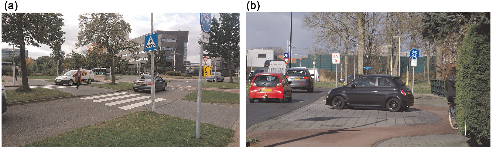
Most crossing traffic, however, is not expected to be anywhere along the road, but only at intersections. In this paper we will take cyclists as example. Cyclists might cross a road with priority. The cyclist stream is relatively easy to split into two directions, left to right and right to left. This is the situation we consider in this paper (see also Figure 1a). For the sake of readability, in the remainder of the paper, we will refer to the (prioritized) crossing stream as cyclist traffic and to the main stream (of which we analyze capacity) as car traffic. Note, however, that the analyses and results are equally valid for other modes.

Figure 1.

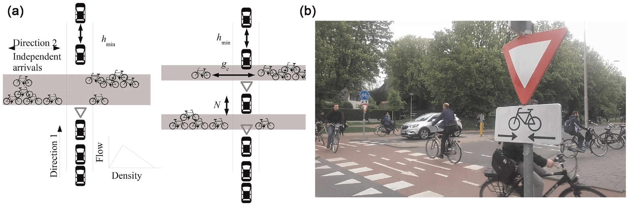
Examples of the situation studied: (a) schemetic representation and (b) example case in Delft, the Netherlands.

This paper therefore studies the effect of separation of cyclist traffic in sub-streams, and is inspired by situations that occur frequently in the Netherlands. An example is shown in Figure 1b. The paper aims to quantify the capacities of the car traffic under various cyclist loads. It distinguishes two situations: (1) all cyclists in one stream, and (2) cyclists in two (or more) sub-streams. The paper also explicitly studies the effect of the distance between the two streams. Intuitively, a separation of cyclists in two sub-streams based on their heading (left–right or right–left) is most sensible. The equations allow any separation, also a simple split of a large cycle crossing right–left into two right–left sub-streams. The paper’s contributions lie in (1) a theoretical contribution on how these computations can be done, including invariant transformations eliminating several variables, and (2) results on the capacities, which can be used (after transformations) as starting point for capacities in practice. Note that these results are obtained on a theoretical basis, and are not empirically tested. This work can be applied at two different levels of design: (1) a single intersection and (2) a network. For an intersection, the method can be applied to split a stream into two or three sub-streams with a space for typically one or two vehicles in between the sub-streams. A larger separation is undesirable because of the increased complexity and the large attention span required of drivers crossing a large intersection. At this level one can also consider the design of combining cycling directions at each side of the road. One can have a bi-directional cycling path at one side of the road, or have a cycle path at each side of the road (one path per direction). At the network level, the design choice is to distribute cyclist traffic over various routes. This will distribute cyclist traffic over various parallel routes. Then, their crossing locations are separated by a larger distance (several hundreds of meters).

Indeed, the paper originates from the Dutch context with already quite a large share of cyclists. More and more often, queuing of vehicles occurs as a result of large streams of cyclists crossings. These streams can consist of thousands and even tens of thousands of cyclists per day. This happens at regular intersections as well as at roundabouts (see for an example of that geometry Figure 7a). Vehicular queuing also impacts the traffic safety, as drivers will become impatient and take larger risks. Also, the blocking might have other severe consequences. Let us give two concrete examples from the Netherlands here. A first is that cyclist traffic blocks the flow into onto a roundabout near a hospital, and as consequence the access route for ambulances into the hospital is somewhat blocked. A second is a cyclist crossing near an onramp of a freeway close to a college. At times near the start of ends of lectures, students cross the road, causing congestion to spill back onto the freeway. In the latter case, priority was changed and cyclists now need to wait for cars. With the methods proposed in the current paper, other solutions could have been tried instead.

The remainder of the paper is set up as follows. The next section presents a foundation of traffic flow theory relevant for the paper. The main traffic flow theory insights are presented there: this shows the symmetries and eliminates some parameters. As a result of the insights from that section, the number of required situations that needs to be studied is largely reduced, to an extent that all situations can be iterated. These remaining situations have been simulated. Both the setup and the results of these simulations are presented in section “Numerical evaluations.” A section on practical application of the insights and the simulation results follows. The final section presents the discussion and the conclusions.

Theoretical Considerations

We consider traffic in two directions. Direction 1 is the traffic for which we are computing the capacity. Direction 2 is the cross-traffic which has priority. The critical gap (denoted $g_c$ ) is defined as the time which is required for a car driver to cross the stream of cyclists. In this paper, we make three assumptions: (1) the critical gap for vehicles in direction 1 to cross a stream is constant (later chosen as $g_c=1$ ); (2) cyclists in direction 2 arrive independently (exponential headway distribution, or Poisson process; a discussion on relaxing this assumption follows later, at the end of the results section); (3) traffic in direction 1 acts according to a triangular fundamental diagram.

Let us first elaborate on the first assumption. Implicitly, we have assumed that the traffic in direction 2 moves in streams with no width. Only when a gap larger than $g_c$ in that stream occurs, a car can move. Realistically, that stream might have a certain width (cyclists moving next to each other, for instance). This would add an (additional) travel time to cross the stream. This can be included into the analyses by incorporating this additional travel time into $g_c$ . It is still required that the stream is empty over the full width, and differences within the width (starting to cross while one side of the crossing is occupied) are not taken into account.

Let us discuss the second assumption. The cyclist blocks the car traffic for a while because it takes time to cross the width of direction 1. The generated headways are gross headways. It can therefore happen that a second cyclist arrives before the first cyclist has crossed the road. In this paper, we do not mention this crossing time explicitly. We specify the critical gap, $g_c$ , as minimum gross time between two cyclists which is needed for a car to pass in between. We therefore move the time to cross the street into the critical gap.

The third assumption means that in uninterrupted conditions the flow of vehicles is (in two branches) piecewise linearly dependent on the density of vehicles ( 11 ). This is characterized by three parameters. In the remainder of the paper, we will use notation free-flow speed $v_f$ , critical density $k_c$ , jam density $k_j$ , critical or capacity flow $q_c$ ( $q_c=v_f{k}_c$ ), and negative wave speed $w$ , defined such that $w>0$ ):

$$w=q_c/(k_j-k_c)$$

(1)

The closest vehicle-to-vehicle headway is $h_{\min }$ , which can be derived from the fundamental diagram by

$$h_{\min }=1/q_c$$

(2)

On a vehicle-level scale, this implies we will use Newell’s simplified car-following model and assume instantaneous acceleration when the road becomes free.

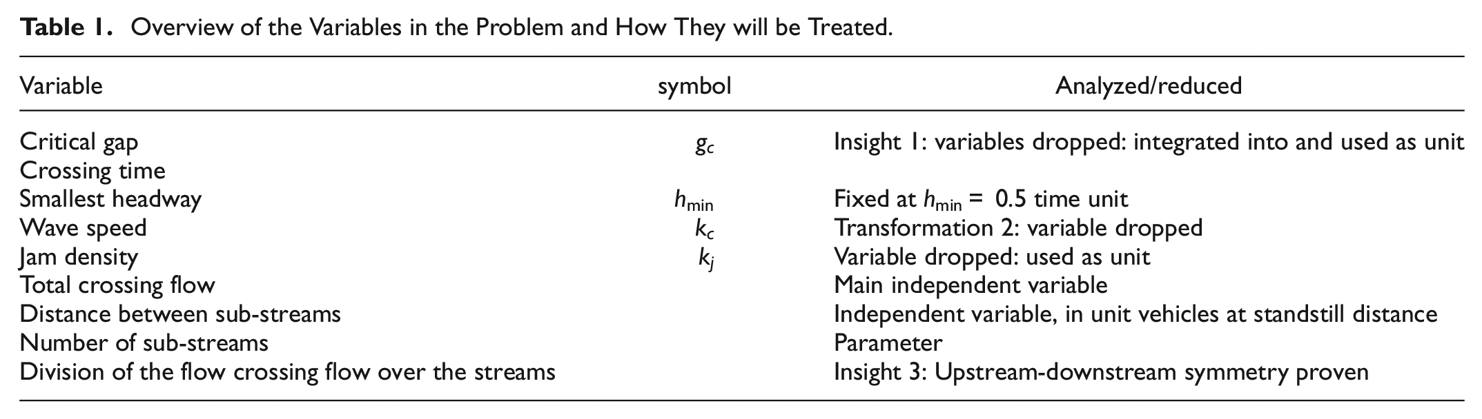
The problem we are facing now is finding the capacity as function of nine variables. These are shown in the first two columns of Table 1. Presenting the flow as function of all these nine variables is not feasible. Therefore, we will introduce a theoretical reasoning and insights to reduce this number. This yields transformations to lose or combine variables. Then a series of simulations can be done by varying all remaining variables, providing capacities. The aim of the transformations is generally that we are able to obtain the results for the capacity for all cases (i.e., variations of all nine dimensions) without the need to redo simulations (but only transformations, which do not need computer simulations). Table 1 first presents (left half) the variables which are in the problem, and presents how these variables are handled (right half).

Table 1.

Overview of the Variables in the Problem and How They will be Treated.

Variable	symbol	Analyzed/reduced
Critical gap	$g_c$	Insight 1: variables dropped: integrated into and used as unit
Crossing time
Smallest headway	$h_{\min }$	Fixed at $h_{\min }$  =  0.5 time unit
Wave speed	$k_c$	Transformation 2: variable dropped
Jam density	$k_j$	Variable dropped: used as unit
Total crossing flow		Main independent variable
Distance between sub-streams		Independent variable, in unit vehicles at standstill distance
Number of sub-streams		Parameter
Division of the flow crossing flow over the streams		Insight 3: Upstream-downstream symmetry proven

The paper will now present the dimensional reductions. Note that the reductions can be done without loss of generality. The insight that these transformations can be done is an important contribution of the paper. They allow us to provide scalable and reusable graphs.

First of all, let us consider the crossing time and the critical gap. Without loss of generality, we rescale time such that the critical gap and the crossing time combined equal 1 unit of time. Depending on definitions, conceptually, one might perceive this combination as critical headway, as it is the minimum time needed between two cyclists for one vehicle to cross. Combining, we define without loss of generality the critical gap accepted $g_c=1$ . Note that the minimum time headway between two successive vehicles $h_{\min }$ is a different variable—generally to be expected shorter.

Second, we will now show that the ratio $w/v_f$ does not influence the capacity, and capacity only depends on the number of vehicles that fit in between the two sub-streams and the uninterrupted capacity $q_c$ (and no other parameters of the fundamental diagram). To show this, we use variational theory ( 12 ) to estimate the capacity. This means we need to construct a (shortest) path in space–time, with edges moving forward at free speed, moving backward at wave speed, or being stationary at blockings. This shortest path determines the capacity, with the cost of that path being the capacity.

Let us recall the transformations introduced by Laval and Castrillón ( 13 ) and Daganzo and Knoop ( 9 ). They show that under stochastic localized blockings, like we have here, the shortest path thus the capacity, is invariant under a skewing transformation of the fundamental diagram, that is, a change of $w/v_f$ . Figure 2a shows an example of the crossings (red lines) and the matching shortest path (blue line) determining the capacity. This is constructed for a fundamental diagram with a high free-flow speed and a lower (negative) wave speed $-w$ , as seen from the slopes of the parts of the shortest path. An additional black dashed line following one of the pieces of the wave illustrates the free-flow speed. Figure 2b shows a modified situation with a different fundamental diagram. The timings of the crossings at $x$  = 2 are modified accordingly. The timing difference makes that the additional black dotted line following the shortest path at free-flow speed intersects with cyclist 2 at the same progress of its crossing. The situation with a modified fundamental diagram and a modified cycle timing (Figure 2b) has the same shortest path as the original situation (Figure 2a), with the same cost, therefore the same capacity. This means, as argued in Laval and Castrillón ( 13 ) and Daganzo and Knoop ( 9 ), that the ratio $w/v_f$ is not influencing the solution. It is important to note here that for both situations, even while the timing of crossings have shifted, the moments of cycle crossing still adhere to the same probability density function before and after the shift.

Figure 2.

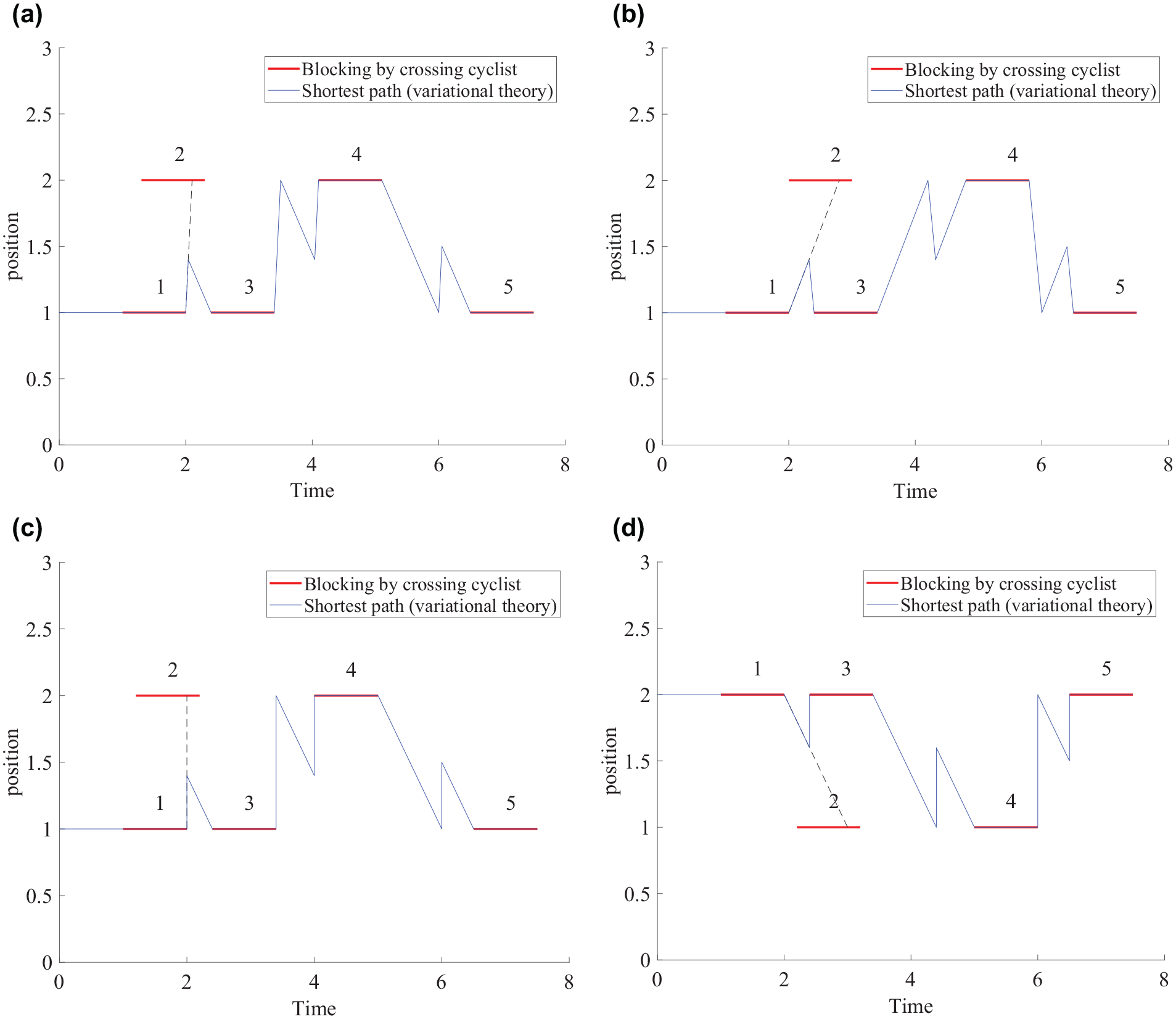
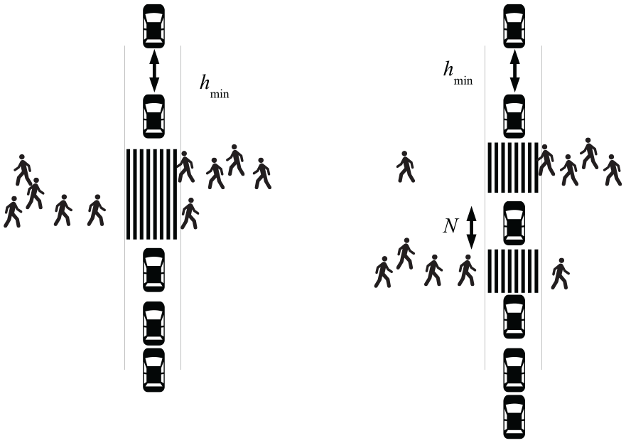
Illustration of the transformation of the cyclist crossing positions and the change of path under inversion of positions and the matching time-shift of the cyclists 2 and 4. Note that the time is scaled such that the blocking has a unit 1 ( $g_c$  = 1); for position, an arbitrary unit can be chosen: (a) higher free flow speed than wave speed, (b) higher wave speed than free flow speed, (c) considered situation for computations, and (d) reversed direction.

Let us now compute the cost for the wave going up and down. We denote distance by the number of vehicles at standstill that fit in between two sub-streams, $N$ ; the following computation will show that this is the only relevant parameter to be considered for capacity. Let us consider a shortest path, and the time this wave takes to travel upstream and downstream. The time moving downstream is then $T_d=(N/k_j)/v_f$ . The time moving upstream is $T_u=(N/k_j)/w$ . The distance between the sub-streams is then $(N/k_j)$ . Adding both times, we find

$$\begin{array}{c}{T}_{\mathrm{all}}=T_u+T_d=N/k_j*(1/v_f+1/w)\hfill \\ =N/k_j*(k_c/q_c+(k_j-k_c)/q_c)\hfill \\ =N/q_c=N{h}_{\min }\hfill \end{array}$$

(3)

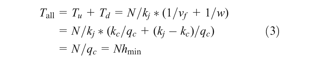
For the rewriting of the above equation, we use substitutions based on Equations 1 and 2.

The total cost in the end equals the uninterrupted capacity $q_c$ times the time $T_{\mathrm{all}}$ . This shows that the time is—as expected—independent on the ratio $w/v_f$ . For the sake of computational simplicity, in the sequel we assume without loss of generality $T_d=0$ and $T_u=N{h}_{\min }$ . (We can justify this because the solution of the problem has just been shown not to depend on $w/v_f$ .) Note moreover that the cost does not depend on another property of the fundamental diagram apart from the uninterrupted capacity $q_c$ . Finally, we observe that for the space between the sub-streams, the number of vehicles in between the sub-streams is the relevant variable.

Third, we show that inverting the order of sub-streams does not influence capacity, even with unequal demands in the sub-streams. This means that, for example, a 40–60 distribution of flow over both sub-streams will yield the same capacity for direction 1 as a 60–40 distribution of flow. This can be explained by the following reasoning: The capacity can be determined using variational theory. For the reasoning behind applying variational theory to traffic streams, we refer to Daganzo ( 12 ). From this paper, we take that the capacity of direction 1 is dependent on the cost of the shortest path in space–time for an observer moving but ending at the same location. An example is given in the space–time diagram in Figure 2. The red lines indicate crossings of cyclists on either of the two crossings, and the blue line is the shortest path. Exactly the same shortest path problem can be found if we (1) invert the order of the crossing cyclists in space (i.e., move them to the other sub-stream), and (2) move the crossings which are now at x = 1 (cyclist 2 and 4 in Figure 2) to a time $T_u$ later (note in Figure 2d, cyclist 2 moves from t = 1.2 to t = 2.2, and cyclist 4 moves also to 1 s later). This new solution also has exactly the same cost, therefore the same capacity.

Summarizing, we can transform one problem to another, with inverted order of sub-streams in a dual coordinate system. Whereas the exact timing of the crossing cyclists is shifted, they are—per sub-stream location—all shifted by the same amount of time. Therefore, the headways (and therefore the headway distribution) of the cyclists is the same. To determine the capacity, one needs to consider an ensemble of realizations of cyclist crossings. Given that the distributions are the same, the two coordinates will yield the same capacities. Therefore, inverting traffic direction or inverting the order of sub-streams will not affect the capacity. This reasoning also applies fully for more than two sub-streams. Note the reasoning is only true for a complete inversion of order, and not for any permutation in case of more than two sub-streams. These three considerations help us in limiting the number of cases that need to be computed to obtain an overview of capacities for all practical cases.

Numerical Evaluations

With the theoretical considerations of the previous section, we have now reduced the number of dimensions over which we need to enumerate to compute all capacities. We can now run simulations to cover a wide range of remaining variables. In this section we first explain how the simulations are run, and then we present the results of these standardized situations. Then, in the next section, it is shown how these standardized results can be transformed back to get results for other cases.

Set Up of Simulation

We compute the maximum number of passings of vehicles by simulating the queuing system under the crossing of cyclists. The simulations are performed for the smallest headway $h_{\min }$  = 0.5, which we consider a typical value. Therefore, we argue that the smallest headway between vehicles in an uninterrupted case is half the gap needed in the cyclist stream to cross. Typically, one can consider a 2.5 s smallest headway and a 5 s critical gap. We consider this reasonable for a short crossing time/crossing distance; the calculations are still correct if they both increase and decrease proportionally (i.e., 3 s shortest headway and 6 s critical gap leads to the same outcomes). We consider crossing flows ranging between 0.1 and 10 vehicles per unit of time (note that this is not an arbitrary unit, but the unit of time is set to the critical gap including crossing time).

We will consider various variations:

1. A varying number of sub-streams (1–3, default 2)

2. A varying split rate (20–80, 40–60, 50–50; default equal over all sub-streams, i.e., 50–50 for two sub-streams)

3. A varying number of vehicles that can fit in between the sub-streams (1, 2, 5, 10; default 1; note that the situation with 0 vehicles fitting in between is captured in the case of one sub-stream)

For variations in one dimension, the other two dimensions are set at the default option, as indicated in the list above. (e.g., if we consider 5 vehicles in between—not being the default of 1—we consider the number of sub-streams to be at the default 2 and the split rate between these streams to be 50–50). In this way, we analyze all of the elements separately.

Cyclist are generated at random times. The flow of vehicles depends on the exact timing of the cyclists. To eliminate effects of stochasticity, we generate a large amount of cyclists, 5,000 for our simulations. For each of the cyclists in direction 2, we therefore have (random) headways. The headways are drawn from an exponential distribution, in line with the assumption of independent arrivals. The cyclists are randomly assigned to one of the sub-streams with a fixed probability. Note that this yields (stochastically) the same result as generating exponential headways at each of the sub-streams with a rate adapted based on the division over the streams. Once generated, they are positioned just upstream of the crossing, and their (future) arrival time is known. Vehicles can cross the stream when the remaining gap to the next cyclist is exceeding the critical gap $g_c$ . If the vehicle passes, the crossing is unavailable for a time equal to the minimum headway between two vehicles $h_{\min }$ . In line with the theoretical assumptions, we assume no travel time from the moment of crossing of the first sub-stream to arrival of the next sub-stream. Note that this time is not being ignored, but it is not needed to account for this time for the capacity computations because of transformation 2: we may assume a fundamental diagram with an infinitely large free-flow speed, and compensate for that by adapting the wave speed.

The flow restrictions caused by the queuing of a downstream intersection are modeled based on the Link Transmission Model ( 14 ). This means that we allow the $(i+N{)}^{\mathrm{th}}$ vehicle to pass a sub-stream not earlier than a time $T_{\mathrm{all}}$ after the $i^{\mathrm{th}}$ vehicles has crossed the sub-stream downstream. In this equation $i$ is an index, and $N$ and $T_{\mathrm{all}}$ are used as in Equation 3.

Results

Figure 3a shows the resulting capacities for direction 1. For all cases, the capacity decreases with increasing cyclist flow, which is as expected. Moreover, all capacities are 2 vehicles (veh) per unit of time for a crossing flow of 0 cyclists per unit of time. This is caused by the choice of $h_{\min }$  = 0.5. Whatever the configuration is, with no flow in the crossing direction, all vehicles follow at their shortest headway, $h_{\min }$  = 0.5, leading to a capacity of 2 veh per unit of time. Let us now consider the various variations.

Figure 3.

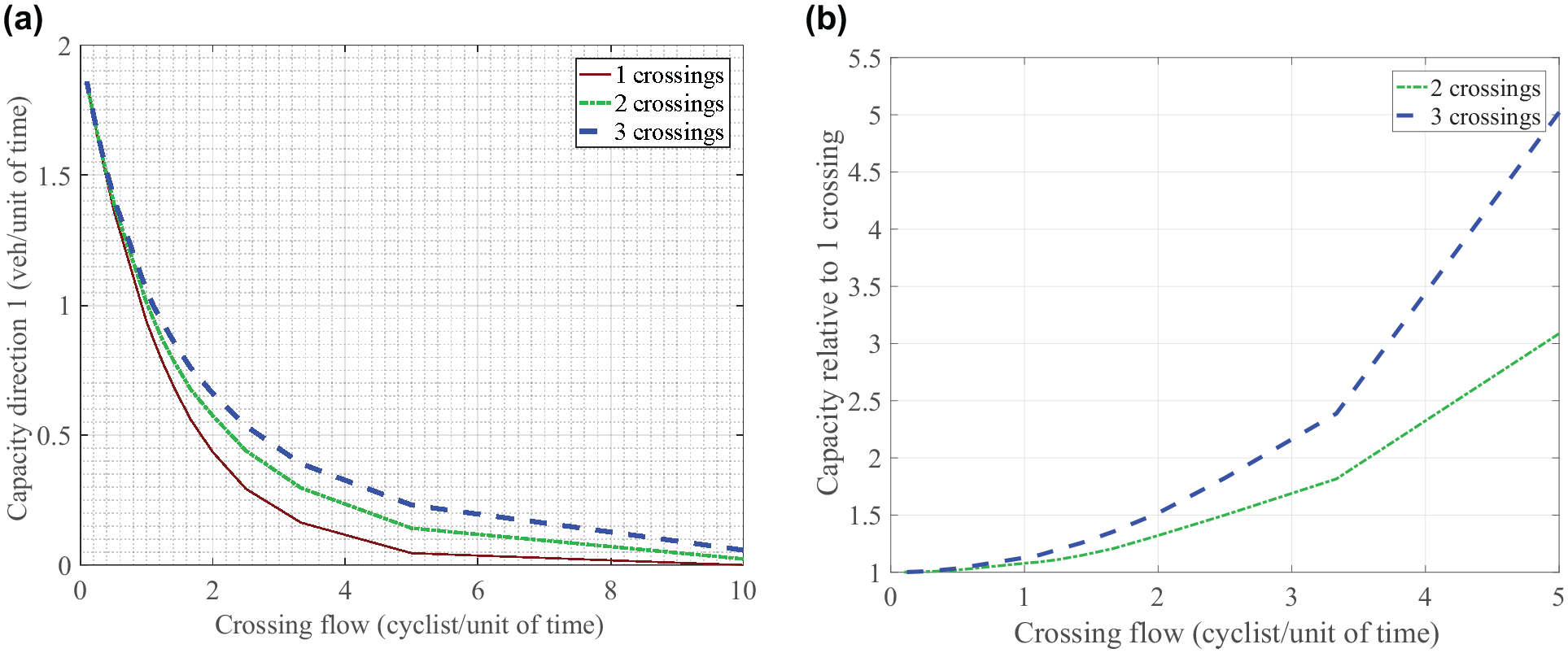
The effect of splitting the stream of cyclist with one vehicle spacing in between: (a) absolute capacities and (b) relative capacities.

First, we consider the effect of multiple sub-streams, see Figure 3a. The capacities relative to one crossing stream are depicted in Figure 3b. For the sake of argument, we went up to three sub-streams. In practice, one or two (sub-)streams are more likely than three. As expected, the capacity decreases for a larger number of crossing cyclists, and increases with increasing number of sub-streams. A first thought might be that for $n$ sub-streams, the capacity is the same as for $1/n^{\mathrm{th}}$ of the stream in one crossing stream. However, this is not true for two reasons. First, stochasticity will always cause one sub-stream to have (slightly) more vehicles, which will therefore be more limiting in capacity. Moreover, and more importantly, there are several sub-streams to cross, which do not operate independently. Therefore, gaps which might be large enough for a vehicle to cross might remain unused because a vehicle (a) cannot enter the buffer space in between because of queue spillback and/or (b) is not present in the buffer space so cannot move forward. This is also the cause of what is called the short block problem ( 13 ). Indeed, that means that a larger spacing in between the sub-streams will lead to a higher capacity, as these elements are not/less restricting traffic flow.

The capacity increases with a larger space in between the sub-streams. This larger space reduces the impact of the limited storage space and/or no vehicles being present in between the sub-streams, as indicated under (a) and (b) above. Figure 4a plots—similar to Figure 3a—the capacity of the car traffic as function of the cyclist flow. In this case, the various lines show how the capacity increases with an increase in the number of vehicles in between. Figure 4b shows the capacities of the situation with a split cross-stream compared with a single cross-stream. It shows that even if only one vehicle can be stored in between, the capacity can triple for high crossing flows. For more vehicles in between, this increases even further.

Figure 4.

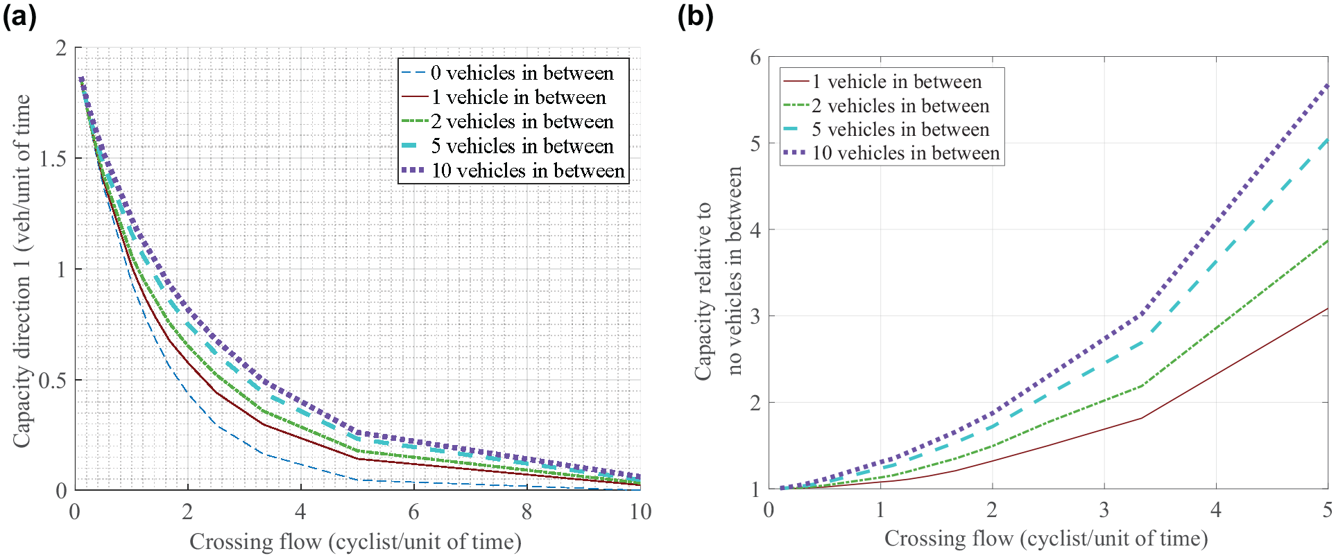
Multiple vehicles in between: (a) absolute capacities and (b) relative capacities.

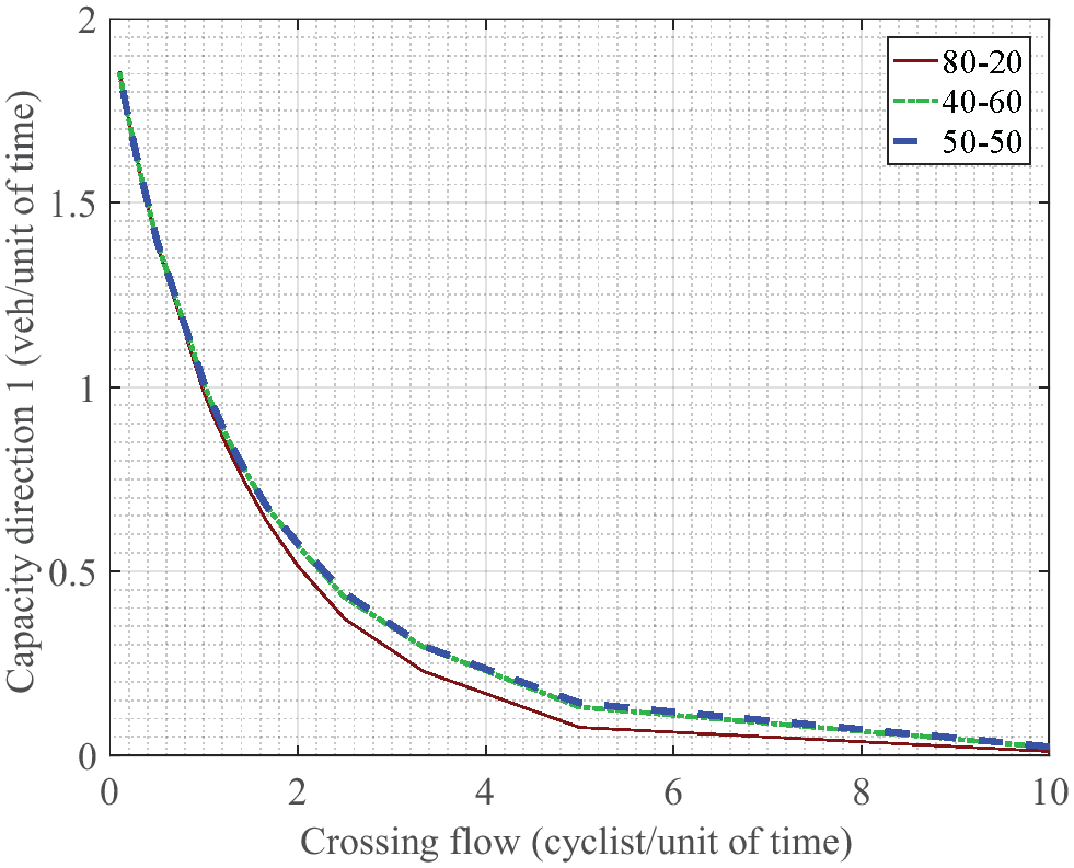
The last consideration shown is the effect of the unequal spread of the flow in case of two sub-streams. As argued in the section “Theoretical considerations,” the capacities for an unequal distribution are independent from the order of sub-streams. This is confirmed by doing simulations for both cases (i.e., 40–60 and 60–40 as well as 20–80 and 80–20). For reasons of simplicity, for each of the pairs we will only plot one line in the graph showing the decay of capacity with increasing flow of cyclist (Figure 5). It is remarkable that a 40–60 distribution has practically the same capacity as a 50–50 distribution for all levels of crossing flows. As expected, capacity reduces further for more biased distribution (80–20).

Figure 5.

Asymmetrical streams.

Discussion

This section discusses the impact of two assumptions; first, the fact of the absolute priority of direction 2. The symmetries between the load on a downstream and upstream sub-streams (i.e., 20–80 and 80–20) hold, given the assumption that the cyclists have priority and can cross. In practice, a queue caused by a downstream sub-stream can grow upstream. In the current paper, we assume that cyclists have priority and find a way to cross (stationary) traffic, even if the queue reaches back to their crossing location. If this is not considered to be realistic, a higher crossing flow downstream will limit the capacity more than a higher crossing flow upstream. Second, in the simulations we have introduced the cyclist with exponential headways. This is the most reasonable assumption, based on independent arrivals. A thought experiment will help considering what would happen for other distributions. Let us consider in this thought experiment the downstream crossing flow to be higher than (or equal to) the crossing flow upstream. We already established theoretically that we can do so without loss of generality because we can invert directions with the same results. This means that the downstream sub-stream is the sub-stream with the capacity constraint, and we should have sufficient vehicles waiting or arriving to use all gaps. We first perform the thought experiment with uniform distributions. In that case, all gaps are equally large, so after the passing of a car, the gap is at least the critical gap. (If the gap would not be large enough, no gap would be large enough, as headways are uniform, and flow would be zero.) As the average inflow from the upstream intersection is at least as high as the outflow from the downstream intersection, there is no possibility that two vehicles can go at the downstream sub-stream and none at the upstream sub-stream, given the uniform arrival patterns of the cyclist. Therefore, it suffices to have one vehicle. Adding storage capacity to two vehicles will not increase capacity. Now consider a distribution with many cyclist following closely (closer than $g_c$ ) and then a larger gap, allowing for N vehicles to cross. Then the maximum flow is reached if the storage capacity allows for N vehicles in between the sub-stream. If the platoon of cyclists is long, there are no vehicles. Intuitively, it can be reasoned that flow is determined by the number of vehicles in the storage. We can find so by considering the limit of very large platoon of cyclists, tending to infinity, with gaps in between these platoons. In that case, the vehicular flow at the upstream intersection is blocked, and only the vehicles in between the intersections can flow. The flow thus fully depends on the storage capacity. Therefore, in that case, the capacity scales linearly with the storage capacity in between, to the maximum determined by N. The insights from the thought experiment is that (a) a different distribution of cyclist flow will change the results, and (b) the effectiveness of the additional storage space above one vehicle depends on the expected size of the gaps compared with the expected size of the time the flow is blocked.

Practical Application

This section elaborates on a numerical example to illustrate how the theoretical insights and the simulation results can be used to solve a practical problem. The last part of the section stresses the wider applicability of the results.

Numerical Example

For this section, imagine one is interested in the capacity of a road with a cycle crossing flow of 600 cyclists per hour in one direction and 900 cyclists per hour in the other direction. For the graphs in the previous section, it has been assumed that the gap that drivers accept between two cyclists is twice the minimum headway between two cars. For the numerical case in this example we assume that a critical gap is 5 s, and thus the road without cyclists has a capacity of 1,440 vehicles per hour (vph) (reasoned from a net time headway of 5/2 = 2.5 s, and therefore a 3,600 s/h/2.5 s/vehicle = 1440 vph capacity).

Now, the crossing flow has to be converted to the natural unit of time used for the graphs, that is, the critical gap, being 5 s here. Doing the conversion, we obtain 600 + 900 = 1500 cyclists/hour = 1,500/3,600 vehicles/s = 1,500/3,600*5 = 2.1 cyclists per unit of time. We now read the graph in Figure 3a; in line with the 600 to 900 distribution of cyclists, we check 40 to 60, and read it at a flow of 2.1 cyclists per unit of time, giving a capacity of 0.54 vehicles/unit of time. As the unit of time is 5 s, the capacity is equal to 0.54(vehicles/unit of time)*3,600(s/h)/5(s/unit of time) = 389 vph.

Other Applications

In this paper, we have considered the case for cyclists crossing a stream of cars, in which the cyclists have priority. The assumptions we made in the theoretical derivations are (as mentioned earlier): (1) the critical gap for vehicles in direction 1 to cross a stream is constant (later chosen as $g_c$  = 1); (2) cyclists in direction 2 arrive independently (exponential headway distribution, or Poisson process); (3) traffic in direction 1 acts according to a triangular fundamental diagram. As long as these assumptions hold, the same analyses can be applied to other cases. In practice, this might be equally true for other cases, for instance for pedestrians which are spread over two pedestrian crossings. Illustrations of these situations are show in Figure 6. Another example is the case where cyclists want to cross a stream of cars and the cars have priority, that is, exactly the opposite situation of what is presented here. In that case, another consideration might be the duration of the crossing and safety for the cyclists. However, the assumption of a triangular fundamental diagram for the main stream (i.e., the pedestrians) might be less accurate, but if one is willing to accept this fundamental diagram, the same computations apply, and therefore the same results can be used.

Figure 6.

Pedestrian crossings.

Also combinations of transport modes are possible, as is shown in some examples from Dutch practice in Figure 7. In one case, shown in Figure 7a, there is a combined pedestrian and cycle crossing with a one-car distance in between. In the other illustrated case (Figure 7b), cars need to cross a stream of cyclists before they merge into a car stream, which also means finding two gaps (one to cross and one to merge into). This is split by moving the cycle path away from the car stream, to a place where a vehicle has the possibility to stand in between the cyclist stream and the car stream. Note that the cycle path bends to the right just before the intersection, and bends back after the intersection. In this case, it also serves the movement of vehicles approaching from the top left side (that direction of the street is not visible in the picture), and turning to their left, that is, into the side street at the right in the picture. They need to cross the car stream in the opposite direction (from bottom to top in the picture which has according to Dutch rules priority over the turning traffic), and subsequently the cyclist stream.

Figure 7.

Examples of cases with a waiting area for a car in between two prioritized crossings (for different modes): (a) Leiden, the Netherlands and (b) Voorschoten, the Netherlands.

Conclusions and Outlook

In this paper we have considered the effect of crossing traffic on the roadway capacity. In particular, we have considered the capacity of the stream which has to give priority to the crossing stream, and the effect of separating the crossing stream into sub-streams. Several transformations have been presented as fundamental insights. The transformations in turn reduce the number of variables and make it possible to enumerate the cases. This paper has presented the graphs for these cases, which in turn can be used to calculate capacities for specific cases.

The methodological insights show us that the relevant parameter is how many vehicles fit in between the two sub-streams. Moreover, we find that for two sub-streams with unequal load, the order of the sub-streams does not matter. Numerically, it is shown that even having room for just one vehicle in between two sub-streams can lead to a capacity that is three times as high as without this possibility. This increase can even exceed three times if the two sub-streams are separated further from each other, that is, with room for more vehicles in between. The capacity curves we have found in this paper can find their way to roadway capacity handbooks.

Even in case of demand levels which are lower than the capacity of the road, there can be travel time delays. Further work should quantify these delays. We believe that the transformations presented in this paper can equally be applied to quantify delays, and are aware that this is yet to be proven. In presenting the results of such a study, a set of graphs like the graphs of capacity might not be sufficient, as delays will depend on inflow, adding another dimension to the results. Visualizing delays might therefore require another approach then a set of graphs.

The insights presented can be transferred to be used in practice. The first step would be to test the insights and find the right values for the parameters used in the scaling. For this, model testing with field data is needed. The current work can be used as prewarning for cases which might need redesign, as well as a rough outline for the possible solutions. It also forms a basis to develop guidelines, which indeed would also need the mentioned empirical testing.