Sage Journals: Discover world-class research

Abstract

Freeway on-ramp areas are susceptible to traffic congestion during peak hours. To delay or prevent the onset of congestion, ramp metering can be applied. A Ramp Metering Installation (RMI) controls the inflow from the on-ramp to the main line so that the total flow can be kept just below capacity. Current ramp metering algorithms apply macroscopic traffic characteristics, which do not entirely prevent inefficient merging behavior from occurring. This paper presents a microscopic ramp metering approach based on gap detection in the right-hand lane of the main line. As preparation for the analyses, trajectory data were collected, by which the mean and standard deviation of driver accelerations were calculated. Simulation, including driver acceleration, is used to test the ramp metering controller. Overall, it shows travel-time savings compared with no-control and compared with existing macroscopic ramp metering systems. Especially during periods of very high main line demand, the microscopic control approach is able to achieve additional travel-time savings. This way, the proposed algorithm can contribute to more efficient road usage and shorter travel times.

Keywords

Operations Traffic Flow Theory and Characteristics ACP50 Traffic Control Traffic Flow

Congestion has been worsening in the Netherlands since 2015 ( 1 ). Congestion causes several undesirable externalitities, such as more traffic accidents ( 2 ), increased pollution levels ( 3 ), and additional travel time ( 4 ). Efforts are, therefore, being made to combat congestion. One example is the implementation of Ramp Metering (RM). The main goal of implementing a Ramp Metering Installation (RMI) is to preserve free-flow conditions on the main line for as long as possible. It has been shown in various studies across several countries that RMIs are successful in prolonging free-flow conditions and delaying the capacity drop by limiting the flow from the on-ramp onto the main line (e.g., Zhang and Ritchie [ 5 ]).

RM algorithms currently implemented are of a macroscopic nature. This is certainly the case in the Netherlands and also elsewhere, as far as the authors are aware ( 6 ). This means that the RMIs reduce the inflow from the on-ramp to levels such that the combined flow from the main line and the metered flow from the on-ramp will not cause congestion. This way, the probability of not having enough room for the merging vehicles to merge smoothly onto the main line is decreased, reducing the probability of congestion emerging ( 5 , 7 – 9 ). This reduces spillback congestion to upstream off-ramps and prevents the so called capacity drop ( 10 ). With the activated RMIs, the average system outflow is, therefore, higher.

Macroscopic algorithms do not search for gaps, but use average macroscopic traffic data to reduce the probability of congestion emerging. A widely researched method to actively search for (and even create) sufficient gaps in merging situations uses Connected and Automated Vehicles (CAVs). The scientific consensus is that deploying only CAVs would lead to less system delay. However, the minimum percentage of vehicles that need to be CAVs to make this work is a subject of debate. Currently, there are hardly any CAVs on the road and it will be some time before there are a significant number. This research aims to develop a traffic control measure that can be used right away, with the currently available infrastructure, which are (dual) loop detectors and traffic lights for the RM control. We will exploit this to search for and use gaps in the traffic stream.

To achieve this, the traffic light shows green to a merging vehicle at such a time that it can be expected that the specific vehicle merges into a specific gap measured in the right-hand lane of the main line. Dual loop detectors can also distinguish between passenger cars and heavy goods vehicles (HGVs). Such an RM control structure that uses microscopic as opposed to macroscopic traffic data will be called a microscopic RM approach in the remainder of this paper. To the best of the authors’ knowledge, no research into the effects of implementing such a microscopic algorithm has been conducted yet. Investigating the quantitative effects of a microscopic RM approach versus the currently used macroscopic RM algorithm in the Netherlands and against a no-control alternative, is the goal of this research to address the aforementioned scientific gap.

The research has been executed by firstly developing a scheme for such a system with only currently used technologies. In other words, only a traffic light and dual loop detectors will be deployed. Dual loop detectors are required to reduce detector noise complications, since the noise now has to include both detectors. For the detectors, only the processing of the data of the detectors has to be changed to obtain individual gaps. No large-scale Vehicle to Vehicle (V2V) or Vehicle to Infrastructure (V2I) communication will be used. Generic development steps for the microscopic control approach scheme are followed ( 11 ). This control scheme will be tested and compared with a no RM alternative and a reference algorithm, which is the current macroscopic RM algorithm in the Netherlands. The simulation program OpenTrafficSim (OTS) is used for this comparison. To achieve realistic simulation runs, accurate acceleration information is required in an effort to simulate the unpredictability of individual drivers. To retrieve this information, trajectory data from real life is collected and analyzed. The outcome of this data collection effort has been used to get a more realistic setting for a microscopic simulation model to test the efficiency of an RMI. When the simulation runs have been executed, the simulation results of the various alternatives can be compared.

This paper will first present the RM algorithms currently used. After that, the newly developed microscopic RM algorithm will be explained. Then, the simulation set-up will be discussed, which is followed by a section on the acceleration experiment. After that, the results are discussed, followed by a sensitivity analysis. The paper ends with discussion points and conclusions.

Ramp Metering Strategies

This section will first discuss RM principles using currently deployed technologies. Then the second half discusses potential strategies involving CAVs. The strategies involving CAVs are used as background information during the development of the microscopic RM algorithm.

As already briefly explained in the introduction, current RMIs are effective in delaying congestion. With RM, the flow from an on-ramp onto the main line is controlled and the optimal flow has to be determined. RM control has already been deployed for some decades ( 12 ) along with multi-level self-learning systems that were first proposed almost 30 years ago (e.g., Liu et al. [ 13 ]). They use macroscopic traffic properties, that is, aggregated quantities like flow or (average) occupancy of a detector. In addition, RM is currently done by using macroscopic traffic characteristics on the main line ( 8 , 14 ). These characteristics are measured by using dual loop detectors on the main line, which measure occupancy, flow, and speed. The average macroscopic traffic characteristics are determined over a small time interval (i.e., the aggregation level). Using the measured macroscopic traffic characteristics and knowledge of the maximum flow possible without causing a congestion, the number of vehicles that are allowed to enter the motorway from the on-ramp can be determined.

The measured macroscopic traffic characteristics can be used in several ways. Basically, one can differentiate between feed-back control structures (which take the effect of their action into account in the new control action) and feed-forward structures (which do not take the effect of their action into account). Typically, algorithms with a feed-back system use loop detectors on the freeway placed downstream of the on-ramp merging area ( 8 ). Algorithms with a feed-forward control use loop detectors on the freeway placed upstream of the on-ramp merging area ( 14 ). Also, a combination of the two can be used ( 5 ). Generally speaking, feed-back control structures are more robust than feed-forward control structures. However, the information that is being used to determine the inflow allowed from the on-ramp always lags behind. Therefore, the same goes for the cycle times of the traffic lights. Using feed-forward control enables the use of the approaching flow to determine the cycle times.

Regardless of the exact control structure, the current algorithms rely on aggregate traffic properties such as flow and speed, so averages are used. Then, vehicles at the on-ramp are not let onto the main line when a gap will be present for them to use, but they will receive a green light every x seconds, based on the difference between the predetermined road capacity and the measured flow. Therefore, it is possible that the merging vehicle will not have a sufficient gap available when going to merge, requiring the merging vehicle to force itself onto the main line. This forceful merging maneuver could lead to a traffic breakdown. So, using average macroscopic traffic data could still lead to a traffic breakdown in a case of an individual merging vehicle not being able to find a sufficient gap to merge smoothly. It can be expected that better results could be obtained (i.e., less travel-time delay) if precisely measured individual gaps in the flow were used to fit merging vehicles in.

In the past, gap-acceptance for ramps has been studied extensively, for example, in 1965 ( 15 ). There is a relation between gaps and macroscopic patterns, as May Jr ( 16 ) points out. More recently, RM on a microscopic level (i.e., controlling individual vehicles to specific gaps) has been researched extensively with the help of V2I and/or V2V communication technologies. For instance, several papers report on strategies on a microscopic level, that is, they aim to link specific vehicles to specific gaps to merge into. These studies are relevant as background material for the development of a microscopic RM algorithm without such communication technologies.

Letter and Elefteriadou ( 17 ) find that in free-flow conditions the developed merging control strategy reduces travel-time delay compared with conventional vehicle operations. The improvement ranged from 3% to 7%. In congested conditions, safety is improved. However, the developed algorithm relies on a CAV share of 100%. Furthermore, this research only uses a single lane main road, which is not common, especially in the Netherlands.

Hu and Sun ( 18 ) do include multiple lanes on the main road. Similarly to Letter and Elefteriadou ( 17 ), complying with the optimized vehicle trajectories results in less travel-time delay compared with a no-control case. The exact reduction in travel-time delay depends on several factors, including the maximum speed, demand split between the main road and the on-ramp, and the demand levels. However, just as in the research described in Letter and Elefteriadou ( 17 ), 100% of the vehicles inside the merging area are required to be CAVs.

Chou et al. ( 19 ) developed an optimization algorithm with V2V communication. They simulate various cases with different percentages of the fleet being CAVs. As expected, the performance of the developed algorithm improves with the penetration rate of CAVs. Additionally, an algorithm which is extended with Infrastructure to Vehicle (I2V) communication technology, is proposed to better cope with conventional vehicles. Although the results are promising, near optimal effectiveness is reached with a penetration rate of 75% or higher. Moreover, the first effects, in the form of less travel-time delay and increased capacity, are shown for a penetration rate of 50%. Both of these penetration levels are still a long way off for the real-life vehicle fleet, let alone a vehicle fleet that solely consists of CAVs.

In conclusion, there is room to improve the macroscopic RM strategies by including microscopic traffic properties. In this paper we want to explore solutions that can be implemented today, without the need for V2I or V2V communication technologies. In an effort to accomplish this goal, this paper develops a new RM algorithm which is based on individual gap measurement by means of currently widely available technologies, such as dual loop detectors.

Microscopic Ramp Metering Algorithm

In this section, we will first present the activation and deactivation criteria for the new RM algorithm and then present the actual working of the RM control algorithm that is based on microscopic gap detection. An overview of detectors and their locations is shown in Table 1, as well as by a schematic picture, illustrated in Figure 1. The table contains the description of the location, which can vary for different on-ramps or countries. For the remainder of the paper, we will refer to the various detectors by their number.

Figure 1.

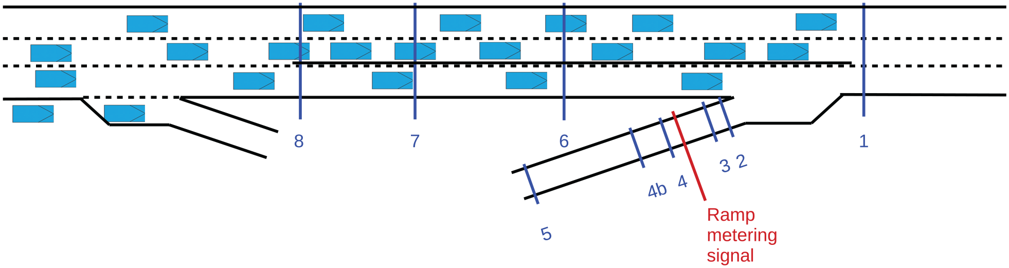
Schematic placement of the detector locations, and layout of the road for the case study. Figure is not to scale.

Table 1.

Detector Locations

Reference number	Detector group	Description	Intended location (Main [M] road or on-Ramp [R])	Vehicle type detection required?	Used in sim?
1	Congestion measurement	Checking if there is a traffic jam just downstream of the merging area.	M: In all lanes of the main road just downstream of the merging area.	No	No
2	Red detection	Checking whether the vehicle has passed the traffic light sufficiently. When triggered the traffic light turns red.	R: Approximately one vehicle length downstream of the stop line at the on-ramp.	No	Yes
3	Yellow detection	Checking whether the front of the vehicle, including the driver, has passed the traffic light. When triggered the traffic light turns yellow.	R: Approximately half a vehicle length downstream of the stop line at the on-ramp.	No	Yes
4	Demand detection	Checking if there is a vehicle waiting at the traffic light.	R: Approx. 2 m upstream of the stop line.	Yes	Yes
4b	Demand detection	Checking if a vehicle is approaching or a second vehicle is waiting. If desired, additional demand detectors could be added.	R: X meters upstream of the stop line. X = one vehicle length + stop line gap + stop spacing.	Preferred.	Yes
5	Congestion measurement	Checking whether the on-ramp is full of vehicles.	R: Near the start of the on-ramp (upstream of the traffic light).	No	No
6	Traffic flow measurement	Measuring the average flows on the main road. When this exceeds a predefined value, the RM control is activated.	M: Exact location depends on the aggregation level and the average speed on the main road. In this research, the location is chosen to be 200 m upstream of the traffic light with a detector across all lanes.	No	Yes
7	Gap measurement detection	Checking if a sufficient gap is present in the right-hand lane of the main road when a passenger vehicle is waiting at the on-ramp. If this detector is not triggered for t seconds, the traffic light will turn green.	M: In the right-hand lane of the main road, y meters upstream of the traffic light. y depends on the average passenger vehicle acceleration, required minimum gap time, and the main road speed. In the base case scenario of this research, this is equal to 334 m.	No	Yes
8	Gap measurement detection	Checking if a sufficient gap is present in the right-hand lane of the main road when a heavy goods vehicle is waiting at the on-ramp. If this detector is not triggered for t seconds, the traffic light will turn green. More of such gap measurement detectors could be included if more vehicle classes are defined.	M: In the right-hand lane of the main road, z meters upstream of the traffic light. z depends on the average heavy goods vehicle acceleration, required minimum gap time, and the main road speed. In the base case scenario of this research, this is equal to 374 m.	No	Yes

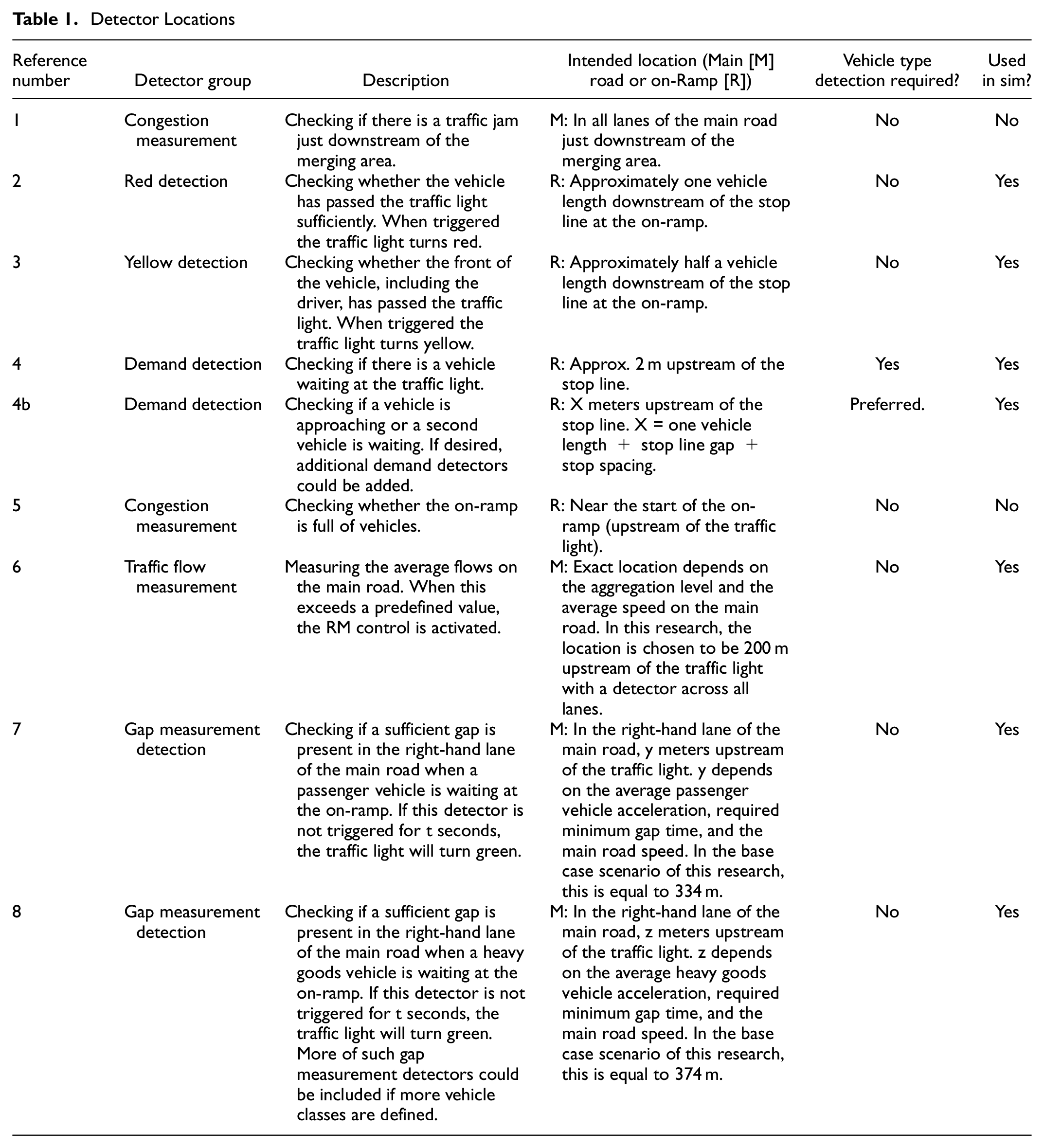
For activation, we choose a threshold flow value and threshold speed value to be measured at detector location 6. If the flow exceeds the threshold value or if the average speed drops below their threshold value, the RMI will be activated. We choose both, since they might indicate different types of congestion. The RMI will be deactivated when both activation conditions are not met or when the on-ramp is entirely filled with waiting vehicles. This additional deactivation condition is introduced to limit spillback congestion on the underlying road network.

The main idea of the control algorithm is to only allow a single vehicle onto the freeway if it is able to accelerate and merge into a sufficient gap in the right-hand lane. To accomplish this, gaps upstream of the merging section are measured and if a suitable gap is detected at location 7 or 8, the traffic light will allow a vehicle to start accelerating. The traffic light allows only one vehicle to pass during a single cycle.

The location of dual loop detectors 7 and 8 is crucial for the success of such an approach. This location should be chosen in such a way that the location of the desired merging maneuver of the controlled vehicle lines up with the measured gap. For this, the following three elements are determined in this order: 1) the time a vehicle needs to accelerate to merging speed; 2) the distance it travels in this time; and 3) the distance the vehicle on the main line travels in this time. This is computed by assuming a constant acceleration, an initial speed of 0 km/h and a desired merging speed as a fraction of the main line speed for the merging vehicles. For the vehicles on the main line, we assume a fixed speed. The location of detectors 7 and 8 is found by subtracting the acceleration distance of the merging vehicles from the distance traveled by the gap.

HGVs will accelerate at a different rate than passenger cars. Therefore, information about the waiting vehicle at the on-ramp is essential. The vehicle class can be distinguished by length via the dual loop detectors, or via detectors that can determine weight with weigh-in-motion or perhaps via number plate identification (in the Netherlands for instance, HGVs have different number plate combinations). Following the aforementioned location determination procedure, locations for detectors 7 and 8 are found. Without further corrections, this might lead to measuring the same gap twice, once for HGVs and then for passenger cars, allowing two vehicles in this one gap. Also, it should be avoid the control algorithm allowing the faster vehicle to enter the on-ramp closely behind the slower accelerating vehicle if the measured gap for the faster vehicle is located downstream of the desired gap for the slower vehicle, implicitly assuming an (impossible) overtake on the on-ramp. To overcome both these issues, a minimum waiting time was implemented if the second waiting vehicle yields a faster acceleration than the first waiting vehicle. This minimum waiting time ( $t_{wait}$ ) is calculated by dividing the difference in the locations of detectors 7 and 8 $(x_{loop}^{slow} - x_{loop}^{fast})$ by the traveling speed of the measured gap ( $v_{main}$ ), added to the required minimum gap time ( $t_{gap}^{slow}$ ), as shown in Equation 1:

t_{wait} = \frac{x_{loop}^{slow} - x_{loop}^{fast}}{v_{main}} + t_{gap}^{slow}

(1)

Combining all these steps results in the complete microscopic RM control structure illustrated in Figure 2.

Figure 2.

Microscopic Control Concept. Detector numbers refer to Table 1 and Figure 1, the latter of which also gives their location.

Simulation Set-up

This section will discuss the simulation set-up. It will first present the site, then how the road properties and the algorithm are modeled in the simulation software. This is followed by the analysis plan, including Key Performance Indicators (KPIs).

Site and Road Properties

The algorithm grants one vehicle access to the main line per cycle. Therefore, a single-lane on-ramp is required. Since three-lane highways are very common in the Netherlands, we aimed for a three-lane section. The A13 Delft-North on-ramp in the direction of Rotterdam fulfills both criteria and was chosen as the considered site. Here, an RMI is already present. At this site, the distance from the traffic light to the beginning of the merging area is 135 m and the length of the merging area is 310 m. The distance between the end of the merging area with the off-ramp upstream of the on-ramp and the beginning of the merging area of the on-ramp is 760 m. This situation has been implemented in the simulation tool OpenTrafficSim (OTS) ( 20 ).

To get the physical road into this package, we designed the following elements. The location of the flow and speed detectors on the main line is the same as the location of these detectors in real life, which is 200 m upstream of the beginning of the on-ramp merging area. These detectors are used not only for the newly developed microscopic algorithm, but also for the reference algorithm. Additionally, an extra loop detector at the on-ramp will be placed to check for upcoming waiting vehicles. The locations detectors 4 and 4b are chosen in such a way that the vehicle will have come to a (near) complete stop when it reaches detector 4, but in case where two passenger vehicles are waiting, both vehicles occupy one detector each. Furthermore, detectors 7 and 8 will check whether a suitable gap is present in the traffic flow. Such a detector is provided for all vehicle classes in the simulation. In this research, detector 7 checks for suitable gaps for passenger cars and detector 8 checks for suitable gaps for HGVs.

The microscopic algorithm is likely to benefit from preventing lane changes from the main line toward the right-hand lane. An asymmetric semi-permeable lane demarcation enabling only one-way lane changes has already been implemented in practice in many cases in the Netherlands. Then, the gaps created by the vehicles taking the off-ramp are not filled by main line vehicles, so the gap can be used by the merging vehicles. Therefore, the base case scenario, which is the starting point of the sensitivity analyses, also forbids lane changes from the center lane to the right-hand lane of the main road for the road stretch between the end of the upstream off-ramp all the way up to, and including, the merging area.

The simulation has two vehicle classes: passenger vehicles and HGVs. We use the default parameters for both classes, except for the maximum acceleration parameter. For the maximum acceleration, a value is used which follows from the empirical study described in the next section. Every single vehicle in the simulation draws a random maximum acceleration from the observed distribution. This distribution differs for HGVs and passenger vehicles.

Analysis Plan

We will compare the algorithm developed here with two other cases. First, there is the no-control case. Second is the reference algorithm, which is equal to the currently deployed algorithm in the Netherlands ( 14 ). The reference algorithm in this research will not only use the locations of the loop detectors as currently deployed at the considered site, but the parameter settings will also be obtained by consulting the recorded specifications ( 14 ).

The traffic input for the simulation runs is the demand per origin–destination (O-D) pair, the HGV fraction, and the speed limit. For the microscopic algorithm, we need to specify the threshold flow, the required minimum gap time and the assumed maximum acceleration. The chosen activation flows consist of the activation flow currently used by the reference algorithm of 1,500 vehicles per lane per hour (vplph) and two increments of an additional 10%. The minimum required gap times are 1.6, 1.8, and 2.0 s. A minimum required gap time of 1.5 or less is not useful in OTS, since vehicles tend to keep a minimum headway of 1.5 s. The assumed maximum accelerations are equal to the mean of the distribution and the value that corresponds with the 37.5th percentile value found in the empirical study.

For the simulated scenarios, the HGV fractions, route demands, and speed limits have to be defined. For the base case scenario, these values are closely matched to the real life situation.

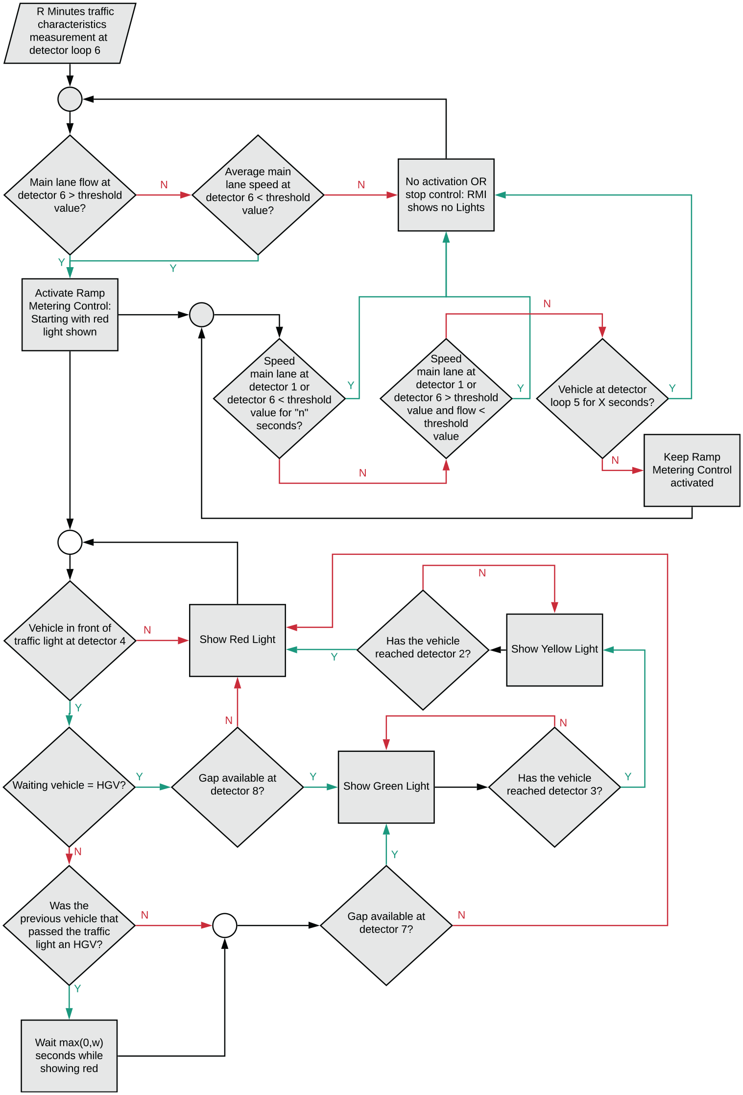
Therefore, for the base case scenario, the HGV fraction for all O-D pairs is set at 5%. Furthermore, the maximum speed limit is based on the real-life situation and the average of the demand patterns is based on logged vehicle intensities at the site. The maximum speed limit is equal to 100 km/h and the corresponding demand patterns in the base case scenario are presented in Figure 3, a and b . As illustrated in the on-ramp and off-ramp demand figure, the average intensities for both ramps are closely matched. This is useful, since vehicles that leave the main road could potentially create gaps for the merging vehicle to merge into. If significantly more vehicles desire to merge onto the main road than leave it, there might be a need for actively creating gaps at the right-hand lane of the main road ( 21 ). The impact of varying the HGV fraction, maximum speed limit and average demands compared with the base case scenario will be noted in the section “Sensitivity analysis” (Table 3).

Figure 3.

Base case scenario demand patterns: (a) base case scenario main line demand pattern; (b) base case scenario main line demand patterns.

The traffic situation is assessed by the average travel-time savings per vehicle in the system for the various alternatives. As a reference for comparing the various microscopic alternatives, we use the no-control base case scenario (i.e., the current situation without an RMI, but with a lane demarcation preventing lane changes from the center lane to the right-hand lane). During the sensitivity analysis, the reference is the single least performing alternative of all investigated sensitivity scenarios. All alternatives are simulated 30 times with different random speeds. This way, stochastic effects will average out and we can compare the averages over these 30 simulation runs to assess design alternatives.

Acceleration Profiles: Empirical Study

The driver model and the parameters used in the simulation tool OTS form a car-following and lane-change model validated with real-world data as described in Schakel et al. ( 22 ). This driver model uses the same fixed acceleration for all vehicles within a single vehicle class. This enables a very precise prediction of the acceleration distance of the merging vehicles. However, drivers within a single vehicle class in real life do not all have the exact same rates of acceleration. In an effort to prevent an overestimation of the effectiveness of a microscopic RM algorithm, the fixed value in OTS should be replaced with more realistic values. The exact acceleration data at RMIs is not yet known and since it is essential for the location of detectors 6 and 7, real-life data have been collected and analyzed to gain insights in the acceleration values in the real world. This section describes the experiment and discusses its outcome.

At the same site as used for the simulation, video footage was obtained by filming with a tripod at the overpass. Vehicles were driving from bottom to top on the screen in the video. All data, raw and processed, are openly available ( 23 ).

From all images, the yellow line of pixels as indicated in Figure 4b is taken. These pixel lines were taken for each frame of the video, recorded at 25 Hz ( 24 ). Then, pixel lines from successive frames were placed next to each other, giving a space-time plot Figure 4a. This plot shows pixels on the vertical axis and time frames on the horizontal axis. One can see stationary objects (stop line, traffic signs, posts) as horizontal lines, since they remain at the same location. Vehicles move from the bottom to the top, creating trajectories which move from bottom to top in Figure 4a. To calibrate space, a researcher drove an identifiable vehicle at a constant speed (66 km/h) through the section (several times). This enables a conversion from the distance in pixels to the distance in meters. The time in frame pixels is converted to time in seconds by using the 25 frames per second ratio that was used for the video. This way, data in meters and seconds can be derived for multiple vehicles.

Figure 4.

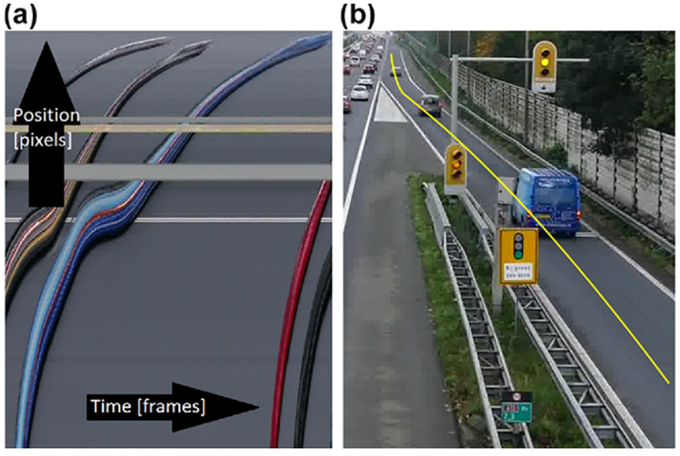
Trajectories and the line of interest: (a) Position, Time (XT) plot; and (b) screen shot with pixel line.

For 16 vehicles, the trajectory was reconstructed by manual extraction of their time at various locations along the ramp. This gives a (quantitative) trajectory of these vehicles from which we will determine the acceleration profile. The acceleration profile will be fitted to a parameterized acceleration profile, consisting of a constant maximum comfortable acceleration ( $a_{\max}$ ) and a dynamic acceleration component, depending on the resistance applied to the vehicle at a certain speed in time and depending on an assumed constant delivered power ( $a_{pused}$ ). Subsequently, the maximum acceleration (needed for the simulations) is a parameter.

For this parameterized acceleration, we assume that vehicles have a constant power for the acceleration trajectory. At low speeds, the constant power would lead to very high accelerations, therefore we assume that acceleration at lower speeds is limited to a fixed maximum comfortable acceleration value $a_{\max}$ . The dynamic acceleration force is equal to the acceleration force minus the resistance force (or drag). For this drag, we only assume the air resistance, expressed by $\frac{1}{2} C_{d} ρ A v^{2}$ , which is by and large the biggest force at higher speeds. The dynamic acceleration force is equal to the power used divided by the speed.

a_{eff} = min {a_{\max}, \frac{\frac{P}{v} - \frac{1}{2} C_{d} ρ A v^{2}}{m}}

(2)

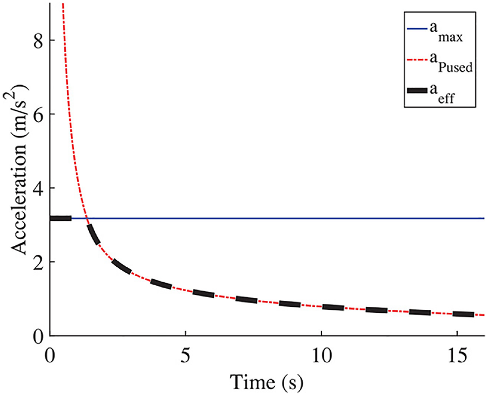
The mass of the passenger vehicles is assumed to be 1,400 kg; for the product of drag resistance coefficients ( $\frac{1}{2} C_{d} ρ A$ ), we assume a value of 1.02 kg/m, derived from a typical modern passenger car. A typical resulting acceleration profile over time is shown in Figure 5, which gives a graphical representation of Equation 2. It shows that the effective acceleration, $a_{eff}$ , for a single vehicle is at the maximum comfortable acceleration at the beginning, and after a while follows a declining dynamic acceleration.

Figure 5.

Typical acceleration profile.

The maximum acceleration ( $a_{\max}$ ) and the power used ( $P_{used}$ ) are calibrated for individual vehicles such that the calculated trajectory is as close to the observed trajectory as possible. These two parameters are found for all 16 reconstructed trajectories. Overall, the fits for the trajectories using this acceleration profile are very good. The average RMSE value in position for all vehicles is 1.1m, with a standard deviation of 0.44. For both these parameters, we fit a normal distribution. The results (mean and standard deviation) are shown in Table 2.

Table 2.

Acceleration Distribution Settings

	$a_{\max}$ [m/s²]		$P_{used}$ [kW]
	Passenger car	HGV	Passenger car
$N_{obs}$	16	-	16 0
Mean	2.02	1.64 (from Rakha et al. [ 25 ])	22.2
Standard deviation	0.60	= 0.60	10.3
Minimum	0.85	0.45	NA
Maximum	3.20	2.80	NA

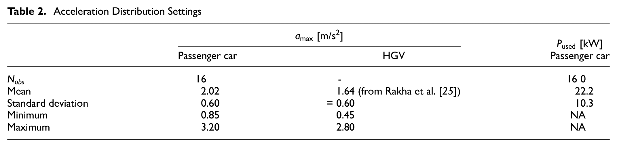
In the simulation, we assign a maximum acceleration to an individual vehicle. This value is extracted from the normal distribution for the parameter “maximum acceleration” from the calibration results. To prevent unrealistically high or low maximum acceleration values, we truncated the normal distribution with a minimum and a maximum value. The extreme values are chosen in such a way that a total of 5% of the distribution is truncated (i.e., 2.5% on both sides of the distribution).

We expect a significantly lower maximum acceleration value for HGVs. In the experiment, we observed many passenger cars, but only a few HGVs. Therefore, another way of setting the distribution for the acceleration value a_max for HGVs is required. To still have a distribution, we adapt the distribution of passenger cars. This is done by changing the mean maximum acceleration to a reference value from Rakha et al. ( 25 ), from $2.02$ m/ $s^{2}$ to $1.64$ m/ $s^{2}$ . For the standard deviation, two changes play a role. HGVs have a lower acceleration, which could result in a lower standard deviation. On the other hand, the (weight) differences between loaded and unloaded HGVs are high, potentially leading to a higher standard deviation. As zeroth order approximation, we assume the standard deviation to be equal to the obtained standard deviation of passenger cars. The procedure for getting a maximum and a minimum value are the same as for the passenger vehicles (i.e., a total of 5% of the normal distribution is truncated).

The number of observations might not be enough to assume these values as the precise real-life values, but it does give an indication of what the acceleration distribution looks like. For this research, the main purpose is to avoid a fixed acceleration value during the simulation runs. Using the observed distribution allows us to avoid using these fixed acceleration values.

Simulation Results

The results of the microscopic algorithm with various sets of parameter values will be presented in this section, see Figure 6. These results entail the average travel-time savings of various runs per combination of settings, labeled in the figure. All considered combinations of parameter settings were simulated 30 times. Therefore, in most cases an average over 30 runs was computed. However, in some rare cases, a vehicle could not reach its destination because of the lack of a sufficiently large gap at the off-ramp upstream of the on-ramp in combination with a vehicle speed that was too low, preventing a successful merging maneuver. When this happened, it occurred before congestion would set in and it would stop the simulation. This happened randomly, and rarely, at most once per combination of parameter settings (out of 30) and only occurred twice in total during the comparison of the various sets of parameter values for the microscopic RM algorithm. These runs were excluded from further analysis since they were not finished, obstructing a fair assessment of the KPIs.

Figure 6.

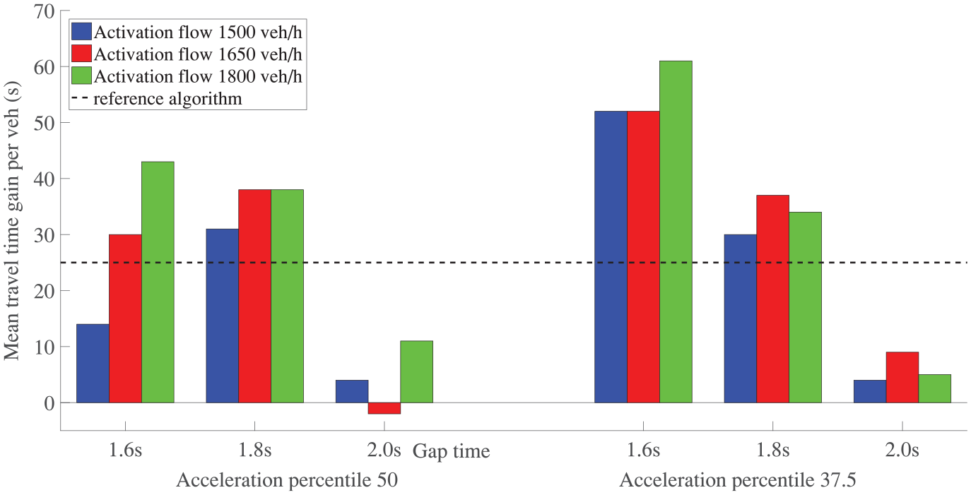
Average travel-time savings in seconds per vehicle, compared with the base case no-control alternative.

Considering Figure 6, two main findings can be derived. We mention these first before elaborating on each of them below:

lower assumed vehicle acceleration values yield better overall results than using the mean acceleration of the distribution for a gap time of 1.6 s;

the average delays for the entire system reduce with smaller gap time settings, especially for the lower assumed acceleration percentile.

On finding 1: the reason that using a lower assumed maximum acceleration results in more travel-time savings for the entire system is because fewer vehicles will have to merge upstream of the measured gap. In fact, if the vehicles do not merge into the planned gap, there are two options. If a vehicle merges in upstream of the planned gap, there is a breakdown probability since that gap might be too small. However, when a vehicle merges in a gap downstream of the planned gap, the new follower of the merging vehicle might reduce speed. Thereby, the new follower will reduce the size of the gap upstream, but since this gap was there in the first place, this has no major consequences for the traffic stream or breakdown probabilities.

For finding 2: smaller gap time settings result in less delay for the on-ramp vehicles and it seems that letting more vehicles onto the main road in the same time frame does not necessarily lead to congestion on the main road with the microscopic RMI algorithm. Thus, the overall average delay for the entire system reduces with smaller gap time settings. It is assumed that the decrease in average delay is a result of the merging vehicles having a gap available to merge into and that a gap of 1.6 s is sufficient.

Sensitivity Analysis

As well as the base case analysis, a sensitivity analysis was performed. Similar to the comparison of the various sets of parameter settings for the microscopic RM algorithm, the alternatives were simulated 30 times for each considered sensitivity scenario. Unfortunately, the same simulation problem of a vehicle not reaching its destination sometimes occurred during these simulations as well. The results of the runs with this problem were removed from the data. Such a simulation problem occurred a total of 13 times over all 1,440 total simulation runs and it happened not more than three times for a single control strategy for one sensitivity scenario.

The scenarios within the sensitivity analysis saw a deviation in the HGV percentage on the on-ramp, the maximum and minimum demand for all O-D pairs and the speed limit on the road. Also, a scenario is tested where the road geometry is changed such that changes to the right-hand lane between the off-ramp and the on-ramp are permitted, effectively resulting in the current situation. The various sensitivity scenarios that were executed are illustrated in Table 3.

Table 3.

Overview of the Simulation Settings

Variable	Base case values	Analyses values
Speed limit [km/h]	100	80; 100; 120
Demand main line	0%	−10%; 0%; +10%
Demand on-ramp	0%	−10%; 0%; +10%
Demand off-ramp	0%	−10%; 0%; +10%
HGV percentage on-ramp	5	0; 5; 10
Possibility to change from center to right-hand lane	not allowed	allowed; not allowed
Parameters setting 1:	asm. acc.: 50%; gap: 1.8s; activation: 1,650 veh/h
Parameters setting 2:	asm. acc.: 37.5%; gap: 1.6s; activation: 1,800 veh/h

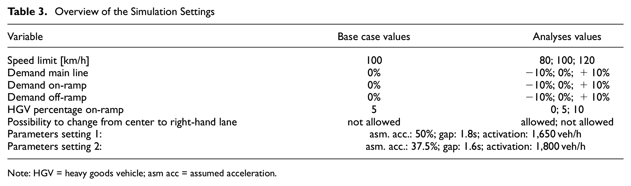
Note: HGV = heavy goods vehicle; asm acc = assumed acceleration.

We simulated the various sensitivity scenarios and we tested the traffic performance using four different RM control settings: 1) ramp metering off; 2) reference algorithm; 3) and 4) the developed control algorithm with two different settings. These settings consist of the best performing combination and a more robust alternative, derived from Figure 6. The more robust microscopic alternative chosen is called microscopic control 1 in Figure 7. The best performing microscopic RM alternative is called microscopic control 2 in Figure 7.

Figure 7.

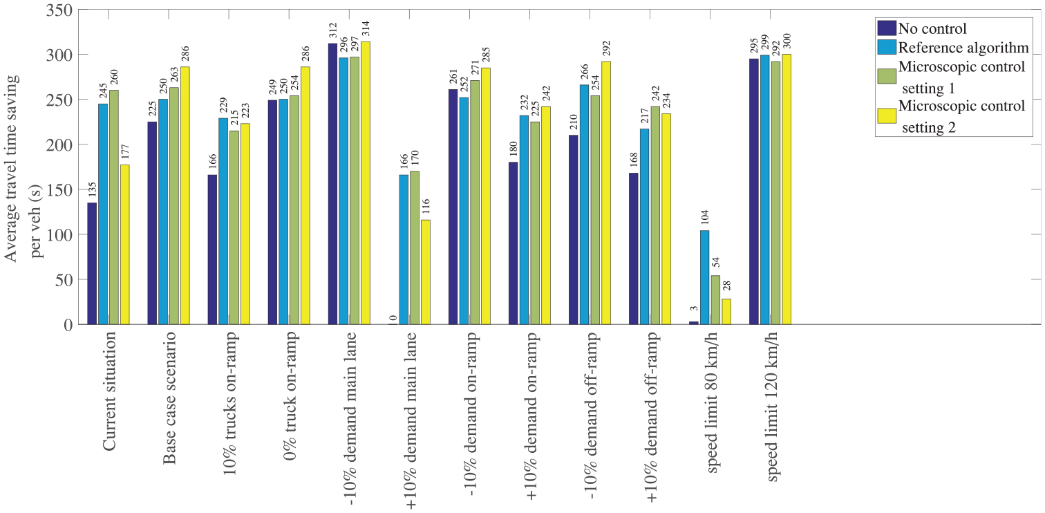
Average travel-time savings in seconds per vehicle, normalized against the no-control alternative with +10% main line demand.

Figure 7 shows the travel-time savings for each of the scenarios. These travel-time savings are compared with the single least performing alternative over all scenarios investigated. For these, we present the travel-time saving results in seconds per vehicle for the entire system. Please note that the number of vehicles can be different in various cases and that analyses with lower speed limits will always result in (more) delay compared with higher speed limits when there is no traffic congestion.

From the results in Figure 7, we conclude the following:

All sensitivity scenarios investigated benefit from a ban on changing lanes from the center lane to the right-hand lane of the main line compared with their counterpart in the current situation;

For some scenarios, the reference algorithm does not attain better overall travel-time savings than the no-control alternative;

The scenario with 10% less main line demand results in much greater travel-time savings for the no-control approach. This is because delays occur when demand exceeds capacity. Such a reduction in demand affects this excessive demand severely, reducing travel-time losses ( 26 );

For all investigated sensitivity scenarios, the proposed control algorithm performs better than having no RMI for at least one of the two settings;

Apart from the speed limit and higher HGV percentage scenarios, the proposed control algorithm performs better than the reference algorithm with at least one of the two parameter settings;

The proposed control algorithm performs better with passenger vehicles at the on-ramp than HGVs, as can be seen from the scenarios with various HGV fractions at the on-ramp.

Conclusion and Discussion

We conclude that the newly developed microscopic RM algorithm leads to less travel-time delay than the reference algorithm in most cases. We do so because: 1) less delay for on-ramp vehicles contributes to fewer delays for the average vehicles over the entire system; and 2) during times of very high demand on the main, the inflow from the on-ramp is higher for both microscopic alternatives compared with the reference algorithm. Moreover, a benefit of the proposed control algorithm is observed compared with not using an RMI. Additionally, the reference algorithm also outperforms the no-control alternative most of the time, which is in line with the literature.

For the scenario introducing a semi-permeable lane demarcation (i.e., the base case scenario), it was found that the microscopic RM control approach could increase the average travel-time savings for the entire system with $13$ up to $36$ s per vehicle compared with the reference algorithm. The reference RM algorithm already saves on average $25$ s per vehicle, making the proposed microscopic RM approaches potentially save either $38$ s or even $61$ s per vehicle compared with the no-control alternative. The exact value depends on the combination of parameter values used for the microscopic alternative.

How much travel time can be saved, depends on several factors. These factors include:

a ban on changing lanes from the center lane to the right-hand lane of the main line;

the speed limit;

the proportion of HGVs at the on-ramp;

the main line, on-ramp and off-ramp demand patterns.

In relation to the ban on changing lanes to the right-hand lane between the end of the off-ramp up to the end of the merging area, it was found that this is beneficial in all investigated sensitivity scenarios, including the base case scenario, and for all simulated control forms. This is, therefore, advisable in all cases (in reasonably heavy traffic demand). The proposed microscopic RM algorithm benefits the most from this ban, since it helps to preserve measured gaps. It thus reduces the probability that a measured gap is filled by another main-line vehicle.

The newly proposed algorithm has benefits compared with the currently used macroscopic reference algorithm in high flow situations, but less so in flows closer to the activation threshold flow. Therefore, an ideal control rule could combine various types of algorithm based on the flow on the main line. The combination and switching rules between the algorithms are a subject for further research.

Some discussion points in the research are still open. First, drivers in the simulation tool (OTS) tend to keep a minimum time headway of 1.5 s all the time. Therefore, no tests are performed with a smaller headway, since this would always result in a measured gap. Depending on the actual minimum time headway that drivers keep, a smaller time headway might yield even better results. Whereas the exact value might differ, qualitatively the same principle is expected in real life. At a certain value for the minimum required gaps, using a smaller time headway in the algorithm would not result in better overall travel-time savings anymore, since all drivers keep a time headway greater than the time headway used in the algorithm. This would result in all headways being considered sufficient gaps, approaching a no-control situation, since every vehicle that approaches the traffic light, would more or less immediately get green, regardless of the precise traffic flow on the main line.

Secondly, the vehicles in the simulation tend to be conservative in their lane-changing behavior, which also contributed to the simulation problems as described in the results section. Besides the presence of these simulation problems, the conservative lane-changing behavior could also be seen in the relative late merging maneuver by the on-ramp vehicles (i.e., they travel parallel to the measured gap for quite some time for no obvious reason) and in the low number of overtaking lane changes. Drivers on the main line tend to lower their pace more easily than drivers in real life when a safe overtaking possibility is present. More (courtesy) lane changes and overtakings would create more gaps, not only for the proposed microscopic algorithm, but also for the other strategies, including not using an RMI. The courtesy lane changes in particular would benefit the other control strategies more than the microscopic alternative. It is expected that they would happen more in these cases, since the proposed algorithm tries to align the merging vehicles with a gap. It should be noted however, that the driver model and the parameters used in OTS form a car-following and lane-change model validated with real-world data as described in Schakel et al. ( 22 ).

Thirdly, the number of passenger vehicles that were used for getting the acceleration distribution is not large (i.e., May Jr [ 16 ]). This means that whereas we could get an indication of acceleration values and a spread, we do not have a reliable estimate. A different standard deviation produced by more observations would affect the predictability of the actual acceleration of the merging vehicles. A smaller standard deviation would probably increase the effectiveness of the proposed microscopic control algorithm. However, there is no expected bias in the standard deviation used because of the limited number of observations. In other words, the low number of observations of the acceleration experiment is likely not expected to influence the effectiveness of the microscopic RM control algorithm.

Nonetheless, the outcomes of this research are promising and it has been shown that a microscopic RM approach can improve traffic operations considerably. There are even some further refinements possible. Besides the aforementioned combination and switching rules between the algorithms, it is currently assumed that the gap on the main line travels at a predetermined speed. Changing this to the actual speed of traffic and then adapting the timing of the green light on the on-ramp based on that speed is likely to improve the share of merging vehicles actually merging into the measured gap, thus improving the overall performance of the microscopic RM approach. Or possibly even more powerful, also in an effort to limit the negative consequences of detector malfunction, a video camera could be used to measure gaps on the main road. If using this camera also enables speed detection, the camera might search for gaps at a dynamic location, depending on the speed on the main road. This could further improve the current algorithm. Additionally, the algorithm can be refined by differentiating between the required gaps for HGVs and passenger vehicles. Lastly, the current set-up is based on a single-lane on-ramp. Investigating the possibilities of extending the algorithm with a second lane at the on-ramp and/or having a weaving section on the main road instead of a conventional on-ramp is recommended for further research.

Footnotes

Author Contributions

The authors confirm contribution to the paper as follows: study conception and design: S.R. Klomp and V.L. Knoop; data collection: S.R. Klomp; analysis and interpretation of results: S.R. Klomp; draft manuscript preparation: S.R. Klomp and V.L. Knoop. Study supervision: V.L. Knoop, H. Taale and S.P. Hoogendoorn; All authors reviewed the results and approved the final version of the manuscript.

Declaration of Conflicting Interests

The author(s) declared no potential conflicts of interest with respect to the research, authorship, and/or publication of this article.

Funding

The author(s) disclosed receipt of the following financial support for the research, authorship, and/or publication of this article: This research was done within the ITS Edulab, a cooperation between Delft University of Technology and Rijkswaterstaat ().

ORCID iDs

Stefan R. Klomp

Victor L. Knoop

Henk Taale

Serge P. Hoogendoorn

Data Accessibility Statement

Data is available at doi:doi.org/10.4121/14791917

References

CBS. Aantal wegvoertuigen blijft stijgen, 2019. https://www.cbs.nl/nl-nl/nieuws/2019/14/aantal-wegvoertuigen-blijft-stijgen. Accessed August 28, 2019.

Barth

Boriboonsomsin

Trafﬁc Congestion and Greenhouse Gases. Access Magazine, Vol. 1.

Calthrop

Proost

Road Transport Externalities. Environmental and Resource Economics, Vol. 11, 1998, pp. 335–348. https://doi.org/10.1023/A:1008267917001.

Theoﬁlatos

Yannis

A Review of the Effect of Trafﬁc and Weather Characteristics on Road Safety. Accident Analysis & Prevention, Vol. 72, 2014, pp. 244–256. https://doi.org/10.1016/J.AAP.2014.06.017.

Zhang

H. M.

Ritchie

S. G.

Freeway Ramp Metering Using Artiﬁcial Neural Networks. Transportation Research Part C: Emerging Technologies, Vol. 5, 1997, pp. 273–286. https://doi.org/10.1016/S0968-090X(97)00019-3.

Middelham

Taale

Ramp Metering in the Netherlands: An Overview. IFAC Proceedings Volumes, Vol. 39, 2006, pp. 267–272. https://doi.org/10.3182/20060829-3-NL-2908.00047.

Kotsialos

Papageorgiou

Middelham

Optimal Coordinated Ramp Metering with Advanced Motorway Optimal Control. Transportation Research Record: Journal of the Transportation Research Board, 2001. 1748: 55–65.

Papageorgiou

Hadj-Salem

Blosseville

J.-M.

ALINEA: A Local Feedback Control Law for On-Ramp Metering. Transportation Research Record: Journal of the Transportation Research Board, 1991. 1320: 58–67.

Rijkswaterstaat. Periodieke monitoring TDI 708004 02-09-2019 t/m 20-09-2019. 1st ed. Ministerie van Infrastrcutuur en Milieu, Rhoon, The Netherlands, 2019.

10.

Yuan

Knoop

V. L.

Hoogendoorn

S. P.

A Microscopic Investigation into the Capacity Drop: Impacts of Longitudinal Behavior on the Queue Discharge Rate. Transportation Science, Vol. 51, No. 3, 2017, pp. 852–862.

11.

Knoop

Hegyi

Salomons

Van Lint

Yufei

Landman

Trafﬁc Flow Modelling & Control. Course Reader. Delft University of Technology, 2019, pp. 389–395.

12.

Goolsby

M. E.

McCasland

W. R.

Freeway Operations on the Gulf Freeway Ramp Control System. Texas Transportation Institute, Texas A & M University, 1969.

13.

Liu

J.-C. S.

Kim

J. L.

Chen

Hao

Lee

Kim

Thomadakis

An Advanced Real-Time Ramp Metering System (ARMS): The System Concept, Vol. 1232. Texas Transportation Institute, 1994.

14.

Rijkswaterstaat. Verkeerstechnische speciﬁcatie van een applicatieprogramma voor toeritdosering. 1.09, Rijkswaterstaat, 2013.

15.

Drew

D. R.

Gap Acceptance Characteristics for Ramp-Freeway Surveillance and Control. Texas Transportation Institute, Texas A & M University, 1965.

16.

May

A. D.

Jr . Gap Availability Studies A Vailahility Studies.The Congress Expressway Surveillance Project, Oak Park Illinois, 1963.

17.

Letter

Elefteriadou

Efﬁcient Control of Fully Automated Connected Vehicles at Freeway Merge Segments. Transportation Research Part C: Emerging Technologies, Vol. 80, 2017, pp. 190–205.

18.

Sun

Trajectory Optimization of Connected and Autonomous Vehicles at a Multilane Freeway Merging Area. Transportation Research Part C: Emerging Technologies, Vol. 101, 2019, pp. 111–125.

19.

Chou

F.-C.

Shladover

S. E.

Bansal

Coordinated Merge Control Based on V2V Communication. Proc., 2016 IEEE Vehicular Networking Conference (VNC), Columbus, OH, IEEE, New York, 2016, pp. 1–8.

20.

Van Lint

Verbraeck

Knoppers

Schakel

Tamminga

Yuan

The OpenTrafﬁcSim Project, 2020. https://opentrafficsim.org/old/index.php. Accessed January 17, 2020.

21.

Subraveti

H. H. S. N.

Knoop

V. L.

van Arem

Improving Trafﬁc Flow Efﬁciency at Motorway Lane Drops by Inﬂuencing Lateral Flows. Transportation Research Record: Journal of the Transportation Research Board, 2020. 2674: 367–378.

22.

Schakel

W. J.

Knoop

V. L.

van Arem

Integrated Lane Change Model with Relaxation and Synchronization. Transportation Research Record: Journal of the Transportation Research Board, 2012. 2316(1): 47–57.

23.

Knoop

Klomp

Freeway Trajectory Recordings: On Ramp Accelerations and Gap Choices After Ramp Metering, 2021. https://doi.org/10.4121/14791917

24.

Knoop

V. L.

Hoogendoorn

S. P.

van Zuylen

H. J.

Processing Trafﬁc Data Collected by Remote Sensing. Transportation Research Record: Journal of the Transportation Research Board, 2009. 2129: 55–61.

25.

Rakha

Lucic

Demarchi

S. H.

Setti

J. R.

Aerde

M. V.

Vehicle Dynamics Model for Predicting Maximum Truck Acceleration Levels. Journal of Transportation Engineering, Vol. 127, No. 5, 2001, pp. 418–425.

26.

Taale

Turpijn

Een fundamentele relatie in coronatijd. Colloquium Vervoersplannologisch Speurwerk, Vol. Corona editie 2020.

Ramp Metering with Microscopic Gap Detection Algorithm Design and Empirical Acceleration Verification

Abstract

Keywords

Ramp Metering Strategies

Microscopic Ramp Metering Algorithm

Simulation Set-up

Site and Road Properties

Analysis Plan

Acceleration Profiles: Empirical Study

Simulation Results

Sensitivity Analysis

Conclusion and Discussion

Footnotes

Author Contributions

Declaration of Conflicting Interests

Funding

ORCID iDs

Data Accessibility Statement

References