Sage Journals: Discover world-class research

Abstract

This article examines enterprise profit rates in key US sectors. Competition between capitals of different compositions modifies values into prices of production to equalize profit rates. These prices of production are further modified into enterprise profit rates when financial payments, rents and interest are treated as a cost. This article applies data from the Internal Revenue Service (IRS) to show that (notwithstanding widely differing technical, value and organic compositions of capital, rates of turnover, proportions of productive and unproductive capital and rates of surplus value) competition tends to equalize profit rates in all sectors barring finance, insurance and real estate. It applies a method that rejects the use of neo-classical, Hulten and Wykoff, fixed capital stock (FCS) estimates (widely used in Marxian rate of profit estimates) as described in the United Nations (UN) System of National Accounts (SNA). This article estimates the overvaluation implicit in the Hulten and Wykoff statistics by sector and develops original sectoral rates of turnover, the organic composition of capital, annual rate of surplus value and enterprise rates of profit from 1994 to 2020.

Keywords

fixed capital advanced fixed capital stock Hulten and Wykoff Marxism rate of profit

Introduction

Marx’s assumption of an equal profit rate is widely questioned within Marxist economics. Emmanuel Farjoun and Moshe Machover (2020) rejected it, explaining that they discarded Marx’s concept of price of production, values modified by competition to equalize profit rates or what they called the ideal price ‘which is the transitional theory interposed between value and market price. We reject it because we think it is an unnecessary, ill-founded, and incoherent fetter on political economy’ (Farjoun & Machover 1985: 105). Paul Cockshott and Allin Cottrell (2003), in one of a series of empirical studies that sought to bolster this assertion, claimed that ‘there is now a substantial body of empirical evidence to indicate that price formation in capitalist economies can be modelled at least as well by simple labour values as it can by prices of production’ (p. 750). Cockshott and Cottrell used data from the UK input-output tables and the 1987 US input-output table along with Bureau of Economic Analysis (BEA) capital stock figures for the same year. They did not have data for turnover times.

Marx’s concept of the price of production, or that equal profit rates are imposed through competition, was common among classical political economists. It arose from the simple observation that all money is equal in the market and so equally deserving of its aliquot share of the capitalists’ collective profit. The capitalist expects all parts of their investment to yield profits equally. This obscures the origin of profit in surplus value or surplus labour, and reconciling this with the labour theory of value was a key discovery of Marx, the solution to Bastiat’s riddle (Marx 1973 [1857–1858]: 385). Indeed

the whole difficulty arises from the fact that commodities are not exchanged simply as commodities, but as products of capitals, which claim participation in the total amount of surplus-value, proportional to their magnitude, or equal if they are of equal magnitude. (Marx’s emphasis, Marx 1959 [1894]: 131)

The exchange of commodities at their values was both historically and logically prior to developed industrial capitalist production. The transition to industrial capitalism meant there was no direct relationship between the surplus value produced in a particular industry or sector and the amount of profit realized in it (Jefferies 2021).

Cockshott and Cottrell’s use of neo-classical fixed capital stock (FCS) valuations is typical of Marxian profit rates estimates, wherein the elision of these Hulten and Wykoff (1981a) valuations with fixed capital advanced is practically unquestioned (Jefferies 2023). Anwar Shaikh treated the valuations in the System of National Accounts (SNA) as if they were valuations of capital advanced. He considered the example of ‘a computer costing $2,000 which lasts 4 years’ to be the capital advanced, the $2,000 past cost of the computer, returned gradually through depreciation. However, neo-classical valuations based on the net present value (NPV) of an asset are not estimates of capital advanced but discounted aggregates of future profits. Shaikh (2016: 801–803) recognized this but treated the two measures as in practice identical, notwithstanding his criticisms of the neo-classical assumption of perfect competition and knowledge. Ironically, Solomon Fabricant (1938: 8–9), who participated in establishing these measures in the 1930s, had observed that NPV measures will only equal costs if there are no profits, or in other words, within perfect competition. Adalmir Marquetti et al. (2010) used Brazilian national accounts FCS estimates to determine a rate of profit. Dave Zachariah (2009) used Marquetti’s Penn World Table (PWT) data to estimate world profit rates, as did Michael Roberts (2020, 2023) and Deepankar Basu et al. (2025). Basu et al. (2025) provided ‘estimates of world profit rates since 1960’ as ‘the rate of profit is one of the key parameters that captures the dynamics of capitalism’ (p. 1). Basu et al. used PWT ‘country-level data on profit income and capital stock’ to ‘compute a world profit rate. In year $t,$ the world profit rate is defined as,

r_{t}^{w} = π_{t} / K_{t}

(1)

where $π_{t}$ and $K_{t}$ are the world net profit income and world capital stock, respectively, in year $t$ ’ (Basu et al. 2025: 4). Basu et al.’s (2025) claimed novelty arose first ‘from the world profit rate being a weighted average of country-level profit rates with a country’s share in the world capital stock being the weight’, and second, ‘we use two different data sources: the latest version of the Extended Penn World Tables (EPWT 7.0) and the Socio-Economic Accounts of the World Input-Output Database’ (p. 2). Basu and Moraitis (2023) similarly used data from the World Input-Output Database that ‘adhere to the 2008 version of the SNA’ (World Input Output Database (WIOD) 2023), to develop a slightly more refined rate of profit estimate. Duncan Foley used the PWT as collated by Marquetti to estimate the fixed capital advanced (K) and the denominator of his rate of profit calculation; the ‘variable K ($/year) is our estimated net fixed standardized capital stock’ (Marquetti et al. 2021). Foley and Marquetti followed the Hulten and Wykoff (1981a) application of the perpetual inventory method (PIM). Marquetti (2021) considered that there are:

two major problems in our attempt to estimate the capital stock that involves strong simplifications. First, the investment data is not presented by categories of gross fixed capital formation and it includes the gross residential capital formation as well as change in stocks. Second, the investment variable is reported for a short period of time. The solution for these problems is to consider not only that all categories of gross capital formation have the same asset life, but also that the asset life is very short.

This did not identify the major problem with the PWT data. The major problem with PWT data is that it transforms an increase in the mass of profit into a fall in the rate of profit. Thomas R. Michl (2023) used the PWT data to derive a rate of profit series which, typical of these estimates, showed a U.S. rate of profit that collapsed from 1995, slumping further through the period of hyper-globalization (2001–2008) and then settling significantly below even the crisis years of 1980–1982. NPV measures grossly overestimate the value of the FCS so that any increase in the mass of profit, the numerator of the rate of profit calculation, will be outweighed by the increase in the denominator, which is the mass of profit multiplied by the service life.

Feenstra et al. (2015) who oversaw the collation of the PWT8 dataset explained in their description of the methods applied in the updated PWTs that ‘for PWT8, we develop a dataset with investment in up to six assets, shown in Table C1 with their geometric depreciation rates’ they continued:

We first distinguish structures, transport equipment and machinery. We do this based on OECD National Accounts, country National Accounts, EU KLEMS (www.euklems.org) and ECLAC National Accounts (Economic Commission for Latin America and the Caribbean) (p. 10)

They added:

for data on investment prices over time, we use EU KLEMS, OECD National Accounts, ECLAC or UN National Accounts. (Feenstra et al. 2015: 11)

The foreword of the United Nations (UN) SNA explained that it provided a statistical framework that was

a comprehensive, consistent, and flexible set of macroeconomic accounts for policymaking, analysis, and research purposes. It has been produced and is released under the auspices of the United Nations, the European Commission, the Organisation for Economic Co-operation and Development, the International Monetary Fund, and the World Bank Group. (UN 2009: Foreword)

It presented the common, established, well-worn, tried, and tested methods still used to create the SNA across all the major statistical bodies in the world today.

The UN explained that their consumption of fixed capital ‘does not represent the aggregate value of a set of transactions. It is an imputed value whose economic significance is different from entries in the accounts, based mainly on market transactions’ (UN 2009: 103). The use of the term consumption of fixed capital is deliberately made so as to distinguish it from depreciation, commonly used in ‘commercial accounting’ to apply to the ‘writing off historic costs’, whereas ‘in the SNA, consumption of fixed capital is dependent on the current value of the asset’ (UN 2009: 123). The OECD (2009) explained that this current value is ‘in a functioning market, the stock value of an asset is equal to the discounted stream of future benefits that the asset is expected to yield’ (p. 30). The Organisation Economic Cooperation and Development’s (OECD’s) manual provides a catalogue of the methods used to construct valuations of the FCS in the various SNAs across the world. It unambiguously explains that all their formulations ‘build on the idea that the price of an asset equals the discounted value of the net benefits that it is expected to generate in the future’ (OECD 2009: 102). This market equilibrium condition forms the conceptual link between the age-price profile and the depreciation pattern.

The central economic relationship that links the income and production perspectives to each other is the net present value condition: in a functioning market, the stock value of an asset is equal to the discounted stream of future benefits that the asset is expected to yield, an insight that goes at least back to Walras (1954) and Böhm-Bawerk (1891). (Author’s emphasis, OECD 2009: 30)

Milton Friedman (1955) commented that Walras’ ‘problem is the problem of form, not of content: of displaying an idealized picture of the economic system, not of constructing an engine for analyzing concrete problems’ (p. 904). Yet Walras’ ideal system is precisely used to analyse the concrete problems, a point that even Milton Friedman did not think it was fit to do. NPV is the ‘value of discounted expected flows of benefits from using an asset in production; equals the stock value of an asset in equilibrium’ (OECD 2009: 231). Benefits were understood as income or the value of capital services generated by the asset (OECD 2009: 30). As this is a neo-classical series, by definition, the market is in equilibrium; only neo-classical markets can be, hence:

The value of a fixed asset to its owner at any point of time is determined by the present value of the future capital services (that is, the sum of the values of the stream of future rentals less operating costs discounted to the present period) that can be expected over its remaining service life. Consumption of fixed capital is measured by the decrease, between the beginning and the end of the current accounting period, in the present value of the remaining sequence of expected future benefits. (UN 2009: 124)

The consumption of fixed capital is a ‘forward-looking measure that is determined by future, and not past, events’ the expected benefits from the assets service life such that ‘the value of a fixed asset at a given moment in time depends only on the remaining benefits to be derived from its use and consumption of fixed capital must be based on values calculated in this way’ (UN 2009: 124).

Marx (1959 [1894]) noted that the capitalisation of ground rent, like every particular sum of money, could be imagined producing an imputed interest and so a value of the asset, using an ‘irrational’ method that aggregates the future rents of an ‘imaginary capital’ in a strikingly similar fashion to that of Hulten and Wykoff:

Ground-rent may in another form be confused with interest and thereby its specific character overlooked. Ground-rent assumes the form of a certain sum of money, which the landlord draws annually by leasing a certain plot on our planet. We have seen that every particular sum of money may be capitalised, that is, considered as the interest on an imaginary capital. For instance, if the average rate of interest is 5%, then an annual ground-rent of £200 may be regarded as interest on a capital of £4,000. Ground-rent so capitalised constitutes the purchase price or value of the land, a category which like the price of labour is prima facie irrational, since the earth is not the product of labour and therefore has no value. But on the other hand, a real relation in production is concealed behind this irrational form. (p. 465)

Robert M. Coen (1978) of the US Treasury Department explained that it was this prima facie irrational form that inspired Hulten and Wykoff as he commented on their original article:

Hulten and Wykoff begin by positing that the value of a building is a function of its age and its date of acquisition. The notion that the age of a building may affect its value is easily understood. Standard capital theory tells us that the value of an asset should equal the sum of the discounted net revenues the asset will generate in the future (net of operating costs but not depreciation). Aging will diminish this value even if net revenue is constant in each year of an asset’s life, because the stream of future net revenues grows shorter. In addition, the asset may lose efficiency or become obsolescent as it ages, in which case net revenue will decline with age and the value of the asset will fall more rapidly. (p. 122)

Capital consumption in the Hultén and Wykoff method is not the depreciation of previously accumulated capital as understood in business accounts, where the cost of past investments is recouped from future sales, but the decline in the NPV of an imaginary capital – the imputed decline of future discounted benefits – in a method akin to the irrational capitalisation of ground rent.

Capital consumption, depreciation, and investment

Aggregated income flows may decline both due to physical deterioration and technical progress, as well as the appearance of new substitutes (UN 2009: 123), but the UN (2009) explicitly states that the ‘depreciation as recorded in business accounts may not provide the right kind of information for the calculation of consumption of fixed capital’ (p. 124). BEA depreciation estimates are not based on fixed capital as recorded in business accounts; rather, the BEA calculates ‘rates of geometric depreciation’ that are ‘based on the Hulten-Wykoff estimates’ (Bureau of Economic Analysis (BEA) 2003: 5; Fraumeni 2000: 14; Hulten & Wykoff 1981b). Fraumeni, for the BEA (published by the OECD), explained:

depreciation is the change in value associated with the aging of an asset. As an asset ages, its price changes because it declines in efficiency, or yields fewer productive services, in the current period and in all future periods. Depreciation reflects the present value of all such current and future changes in productive services. (Fraumeni 2000: 8)

The annual depreciation (the decline in the rate of profits/interest/rents/services/benefits yielded from investments) multiplied by the period of depreciation gives the total depreciation which equals the discounted services it yields. The OECD confirmed that the ‘value of this asset at the beginning of period t, $P_{0}^{t}$ , to its owner corresponds to the discounted stream of future incomes generated by the asset’ (OECD 2009: 30). Hulten and Wykoff developed geometric patterns of the decline of these future services:

We define economic depreciation as the fall in an asset’s price as it ages. Following Hotelling (1925), Hall (1968), and Jorgenson (1974), we assume efficient and competitive capital markets in which, under perfect certainty, the acquisition price of an asset will equal the present discounted value of the future flow of after-tax user costs, inclusive of tax credits and depreciation allowances, up to retirement plus the present value of any retirement value of the asset. (Hulten & Wykoff 1978: 95)

Profit ( $π$ ) is the difference between sales $(M^{'})$ and costs $(M)$ $(M^{'} - M = π)$ , yet for Hulten and Wykoff, confusing enterprise profit with aggregate profit, profits are the net cost of capital or, more accurately, the opportunity cost of capital. This so-called ‘cost interpretation’ of profits underpins the FCS valuations of the UN and OECD (2009),

thus, gross operating surplus per asset – the income flow generated by it – can also be given a cost interpretation: more specifically, it corresponds to the unit user cost of the asset . . . these are in fact the unit user costs, or the price of capital services for the asset . . . which had been labelled $C_{0}^{t}$ . (p. 31)

The valuation is extended for all years of the asset’s life, not only in the year of installation but every year:

When the sequence {ct} is interpreted as a sequence of unit user costs or capital services prices, equation (1) can also be interpreted as a rule for cost allocation over time: the value of a new capital good has to be distributed over accounting periods because of its nature as an investment good. This allocation in time should be such that costs in future periods match capital services that are provided by the asset in each period and measures for quantities and prices of capital services fulfil exactly this role. (OECD 2009: 31)

Surplus is the opportunity cost of an investment, so that perversely, the cost of the asset is the income or surplus or profit generated by it, so if profit is the difference between price and cost, and if cost is profit, then profit is the difference between profit and profit; so profit is the difference between itself and itself. Thus, there is no price, no cost nor profit. Leontief had criticized ‘Irving Fisher’s contraposition of capital and income’ in his PhD dissertation on the circulation of capital; however, this was dismissed by his PhD supervisor von Bortkiewicz as ‘largely misguided’ (Bjerkholt 2016: 37). As Fisher was the President of the Econometric Society overseeing the development of the U.S. SNA, the income measures of capital were used. Joan Robinson (1953) explained this tautology in her critique of neo-classical values of the FCS during the Cambridge Capital Controversy. The OECD’s (2009: 102) Measuring Capital confirmed ‘a possible circularity when the rate of return is computed endogenously’ as ‘a rate of return is needed to compute the age-price profile and hence depreciation. But the rate of depreciation is needed to compute the endogenous rate of return’. This can be solved by a system of nonlinear equations, or more pragmatically, the rate of profit can be given exogenously at a certain ‘plausible’ rate, or in other words, a made-up number. Data about the future is a fiction, a contradiction in terms.

Hulten and Wykoff (1981a) derived asset values are based on a notional rental cost, where costs are equivalent to imputed rents paid to their owner; hence, ‘in equilibrium, the productive efficiency of an s-year-old asset relative to a new asset is equal to the relative rental price ratio’ (p. 368). Implicit rental prices of each asset are used, notwithstanding that assets are owned by capitalists and not rented (BEA 2003: M-3). Hulten and Wykoff (1981a) tested their depreciation schedule using ‘actual market transaction prices of used capital assets to obtain our estimates’ (p. 369). Through examining prices in the secondhand market, they derived capital consumption estimates for the decline in services from the asset. They then multiplied these by the service lives of these assets, which are significantly longer than the depreciation period. In effect, they aggregated rents accrued through ownership rather than costs of capital advanced to derive their valuations of the FCS. The BEA uses real data based on second-hand asset prices that represent ‘plausible’ aggregates of future income flows; a real procedure to produce a fictional number of estimated future rents. The PIM is the most widely used measure of stocks and flows of fixed assets that it ‘rests on the simple idea that stocks constitute cumulated flows of investment, corrected for retirement and efficiency loss’ (OECD 2009: 88), hence:

conceptually, market forces should ensure that the purchaser’s price of a new fixed asset is equivalent to the present value of the future benefits that can be derived from it. Given the initial market price, therefore, and knowledge of the characteristics of the asset in question, it is possible to project the stream of future benefits and continually update the remaining present value of these. This method of building up estimates of the capital stock and changes in the capital stock over time is known as the perpetual inventory method, or PIM. (UN 2009: 125)

The PIM adjusts the value of the FCS, or the aggregate totals of expected future income streams. Different schedules of depreciation are used by various agencies such as the BEA and Bureau of Labour Statistics (BLS), but these are different measures of the change to future services generated by the asset, not measures of the capital advanced. As in aggregate, different rates and periods of depreciation for individual capitals cancel each other out, these schedules are moot; the valuations or aggregates of future services that form them are common to all the statistical agencies. Similarly, investment flows are adjusted accordingly to be consistent with these valuations—‘the estimates of investment underlying the estimates of net stocks are developed to be conceptually and statistically consistent with the NIPA estimates of investment as well as with the classifications of the SIC’ (BEA 2003: 6). These capital indices ‘constructed in a similar way are used in studies by Edward F. Denison, John W. Kendrick, and Dale W. Jorgenson’ (BEA 2003: M-3). Jorgenson (1974) notes that ‘capital stock is the sum of past acquisitions of capital goods weighted by their current relative efficiency given by the sequence ${d_{r}}$ ’

K_{t} = \sum_{r = 0}^{\infty} d_{r} A_{t - r}

(2)

The price of acquisition of a capital good is the sum of future rental prices of capital services, weighted by the relative efficiency of the capital good.

P_{A t} = \sum_{r = 0}^{\infty} d_{r} P_{K,_{t + r + 1}}

(3)

Depreciation on a capital good $P_{D t}$ is a weighted average of future rental prices of capital services with weights given by the mortality distribution.

P_{D t} = \sum_{r = 1}^{\infty} m_{r P_{K,} t + r}

(4)

(Jorgenson’s emphasis, Jorgenson 1974: 205, 206)

Capital advanced is an amount of past capital tied up in production; it may be valued at its installation price, historic price, or its reproduction or replacement current cost, but it is not an estimation of future profits, however valued. Hulten and Wykoff FCS valuations are not an estimate of capital advanced, but a tautological, logically incoherent, irrational valuation of an imaginary capital that aggregates future profits to the present.

Capital advanced the Internal Revenue Service alternative

Marx noted that the ‘cost to the capitalist consists in the capital he advances—in the sum of values he expends on production—not in labour, which he does not perform, and which only costs him what he pays for it’ (Marx’s emphasis, Marx 1972 [1863]: 74). Capital advanced consists of the circulating and fixed capital the capitalist must pay the actual costs they incur (not opportunity costs) for production to take place (Marx 1956 [1885]: 15). Capital is advanced until the circuit of capital accumulation, or reproduction, is complete when money returns to the capitalist from sales. Hence, money returned is not tied up and so is no longer advanced. This capital advanced exists in two forms: circulating and fixed capital. Circulating capital (labour and raw materials) is used up every cycle and so returns to the capitalist after every turnover; fixed capital (machinery, buildings, etc.) returns to the capitalist over many turnovers through depreciation a bit at a time. In a given period, say a year, the capitalist’s circulating capital turns over several times. Hence, the aggregate of these advances of circulating capital in a year is far higher than the cost to the capitalist who only has to advance the money capital for the first turnover, as part of the turnover then pays for these subsequent costs. Whereas fixed capital is tied up longer, it is slowly returned to the capitalist by depreciation over many turnovers. The total amount depreciated is defined by the past capital advanced, not the future profits the investments yield.

The Internal Revenue Service (IRS) measure of Depreciable Assets Less Depreciation (DALD) is the closest official agency category to that of Marx’s fixed capital advanced. The IRS’s figures are a measure of real business expenditures on fixed capital less aggregated depreciation. It values actual amounts of fixed capital advanced, that is, fixed capital tied up in production. Depreciable assets (DAs) are

the end-of-year balance sheet where the book value of tangible property subject to depreciation (such as buildings and equipment with a useful life of one year or more). In general, depreciable assets represent the gross basis amounts before adjustment for accumulated depreciation. (Author’s emphasis, IRS 2005)

While the accumulated depreciation is ‘the portion of depreciable assets written off in the current year and all prior years’ (IRS 2022). The IRS defines fixed capital by time annually, requiring it to last more than 1 year, rather than like Marx, who considers it more than one turnover; however, given that measures of the rate of profit are annual, this distinction is not fundamental. In their ‘Topic No. 704 Depreciation’, the IRS (2022) explained that DAs are:

The kinds of property that you can depreciate include machinery, equipment, buildings, vehicles, and furniture. You can’t claim depreciation on property held for personal purposes . . .. 1. It must be property you own. 2. It must be used in a business or income-producing activity. 3. It must have a determinable useful life. 4. It must be expected to last more than one year. 5. It must not be excepted property. Excepted property (as described in Publication 946, How to Depreciate Property) includes certain intangible property, certain term interests, equipment used to build capital improvements, and property placed in service and disposed of in the same year.

Critically, the IRS measures do not include intangible assets defined as ‘the total gross value of goodwill, contracts, copyrights, formulas, licences, patents, registered trademarks, franchises, covenants not to compete, and similar assets that were amortizable for tax purposes’; these are securities, fictional capital in general, loans, shares, etc., or land. It similarly excludes depletable assets (DPAs; not DAs) defined as ‘the gross end-of-year balance sheet value of mineral property, oil and gas wells, other natural deposits, standing timber, intangible development and drilling costs capitalized, and leases and leaseholds’ (IRS 2022). The conflation of different forms of surplus value, profit, interest, and rent precisely formed the starting point for Hulten and Wykoff values of the FCS.

How much do the SNA overvalue the FCS?

The IRS data is only published in spreadsheet form from 1994 to 2020 (although it is available in PDFs from 1964). The data is largely consistent but the labelling changes. The most comprehensive data set, including assets from 1994 to 2014, is given in Table 6 – Balance Sheet, Income Statement, Tax, and Selected Other Items, by Major Industry, Tax Year, from 2014 to 2020; the same data are relabelled as Table 5.1: Balance Sheet, Income Statement, Tax, and Selected Other Items, by Minor Industry, Tax Year. The data presented here has been corrected as far as possible to overcome these problems (Jefferies 2024).

IRS Total Assets include cash, accounts receivable and payable, inventories, government debt, tax-exempt securities, loans to stockholders, mortgages, other investments, DAs, DPAs, land, intangible assets, and other assets and are a mixture of fictional interest-yielding debts and securities, securitized rent and real capital not fixed capital advanced. The IRS’ Total Assets are generally larger than the SNA’s fixed-asset valuations by some multiple on average for Total Historic Net Private Assets (1994–2020; 348%) and for SNA Current Net Private Assets (216%), but IRS Total Assets are explicitly not an estimate of the FCS. The IRS’ Depreciable Assets Less Accumulated Depreciation (DALD) were on average 7% of Total Assets for the same period, while DPAs, which as has been previously explained are securitized ground rent, were just 1% of Total Assets and Depletable Assets Less Depletion (DPALD) where on average 0.3%.

The SNA’s historic FCS valuation (aggregates of discounted future revenues at the time of purchase) is lower than its current FCS valuation (aggregates of discounted future revenues at present), so current rather than historic valuations are the SNA’s preferred measures of FCS valuation. From 1994 to 2020, BEA Total Historic Net Private Assets were on average 427% of the IRS’ All-Industry DALD, while BEA Total Current Net Private Assets were on average 688%. If SNA current stock FCS valuations are used in a rate of profit calculation, the distortion will be larger by some multiple of historic valuations.

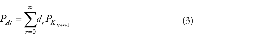
Figure 1 compares the SNA’s estimates of Private Sector Historic Net Fixed Assets with the IRS’ DALD, in mining, construction, agriculture, forestry, fishing and hunting; transportation and warehousing; wholesale and retail trade; manufacturing; and all industries, as defined in the Standard Industrial Classification (SIC) codes.

Figure 1.

BEA/IRS FCS/DALD key sectors 1994-2020.

There are striking variations between the sectors. As BEA valuations are discounted future revenues, they would only equal costs if there were no profits. Finance where profits are interest and speculative gains, real estate and rental and leasing (not included in this figure due to the scale) had an SNA valuation which averaged around 42 times the DALD between 1994 and 2020 and show the largest difference between the DALD and the SNA’s valuation of the FCS. Mining, which combines absolute and relative ground rent and where prices fluctuate due to scarcity, shows SNA valuations fluctuating between five and seven times the DALD. The total private fixed sector is between four and five times, as it includes those sectors that yield rents and interest. Agriculture, forestry, fishing, and hunting, which also yield ground rent, are around four times; transportation and warehousing are around two to three times. Wholesale and retail have been falling from around twice to one and a half times, as DALD increased presumably due to the expansion of warehousing with online purchasing. Manufacturing, despite having a substantial proportion of DALD, rose from around 1.2 to 1.6 times. While construction has the lowest difference at around 1.1 times. In every sector, the use of SNA figures overestimates the value of the FCS, often grossly, and so if used in a rate of profit calculation, it underestimates the rate of profit, sectoral and national, often grossly.

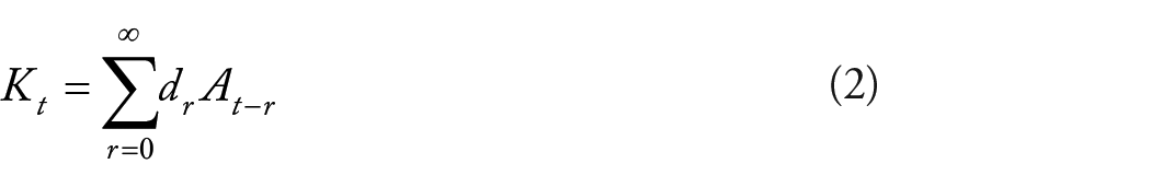
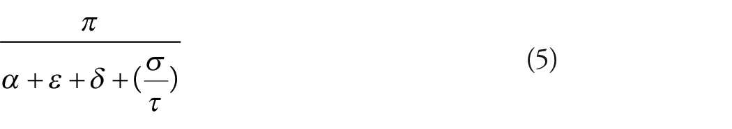
Enterprise rate of profit formula

The division of capital by sectors allows the estimation of the profit of enterprises. Marx (1959 [1894]) observes that:

The actual specific product of capital is surplus-value, or, more precisely, profit. But for the capitalist working on borrowed capital it is not profit, but profit minus interest, that portion of profit which remains to him after paying interest . . . that portion of profit which falls to the active capitalist appears now as profit of enterprise, deriving solely from the operations, or functions, which he performs with the capital in the process of reproduction. (p. 254)

Profit of enterprise is the profit accruing to the capitalist after the payment of interest to the financier. The IRS Balance Sheet categories enable the estimation of sectoral profits of enterprise 1994–2020, for the first time. Turnover ( $τ$ ) is the Net Operating Cycle (NOC) or Cash Conversion Cycle (CCC), the period in days for money spent on inventory or wages to return to the capitalist in cash through the cycle M. . .C. . .P. . .C’. . .M’ (for a detailed explanation of the method to derive turnover, see Jefferies 2023). Profit ( $π$ ) is the Net Income Less Deficit (NILD), while fixed capital advanced ( $α)$ is DALD + circulating capital which is the total of Inventories ( $ε)$ , unproductive capital (Total Deductions (TD) – Cost of Goods Sold (COGS)) ( $δ$ ) + productive circulating capital (COGS) ( $σ)$ /turnover ( $τ$ )) (as only that part of circulating capital directly involved in production turns over). The aggregate of these costs forms capital advanced, the denominator of the rate of profit calculation:

\frac{π}{α + ε + δ + (\frac{σ}{τ})}

(5)

The profit rate formula for all industries and the various sectors appears identical, but there is a crucial distinction between them. What is true of the individual industry or sector is not true for all industries. The aggregate social capital is equal to the ‘sum of individual capitals’, hence, the ‘annual commodity-product (or commodity-capital) of society is equal to the sum of commodity-products of these individual capitals’; however, ‘the form in which these component parts assume in the aggregate social process of reproduction is different’ (Marx’s emphasis, Marx 1956 [1885]: 225). To avoid the fallacy of composition that underpins the neo-classical conflation of profit and cost, it is critical to remember that at the level of All Industry, output is divided into Department one means of production and Department two means of consumption, with exchanges within and between them such that expenditures for one form revenues for the other. The ‘annual value product’ is ‘equivalent to the annual wages received by the working class and the surplus-value annually provided for the capitalist class’, but the mistake is to equate:

the value of the annual product to the newly produced annual value. The latter is only the product of labour of the past year, the former includes besides all elements of value consumed in the making of the annual product, but which were produced in the preceding and partly even earlier years: means of production whose value merely re-appears – which, as far as their value is concerned, have been neither produced nor reproduced by the labour expended in the past year. (Marx’s emphasis, Marx 1956 [1885]: 230)

Aggregate costs and profits are resolved into wages and surplus value, plus value from previous years (depreciation and change of inventories), to form the Annual Value Product (for a more detailed explanation for the estimation of an all-industry profit rate, see Jefferies 2023).

The rate of turnover, ratio of fixed to circulating capital and productive and unproductive capital, the annual rate of surplus value and the equalization of the enterprise rate of profit

The transition to developed capitalist production masks the origin of value and profits in productive labour. Differing compositions of capital, rates of turnover and surplus values mean that prices now fluctuate around modified values or prices of production. The competitive struggle of capitalists to maximize profit rates from all parts of their investment tends to establish a cross-sectoral average enterprise rate of profit.

Sectoral turnovers and circulating capital advanced

Circulating capital advanced is determined by the aggregate of circulating costs, the rate of turnover, and the proportion of unproductive and productive circulating capital. The NOC/CCC can be negative if consumers pay for their purchases in advance or at the point of consumption, as is typical of transport and warehousing and the service sector (a combination of productive services, like private healthcare, film, waste management, and restaurants and unproductive services like law), where production and consumption occur simultaneously. This is shown here as 0 turnover. Where turnover is negative, capital does not have to be advanced for productive circulating capital; rather, the cost of circulating capital is solely a deduction from profits.

Figure 2 Sectoral Turnovers confirm a strong cyclical component, as demand increases, for example, during the run-up to the boom of 2005–2008, the rate of turnover increases, in turn increasing the annual rate of surplus value and the rate of profit.

Figure 2.

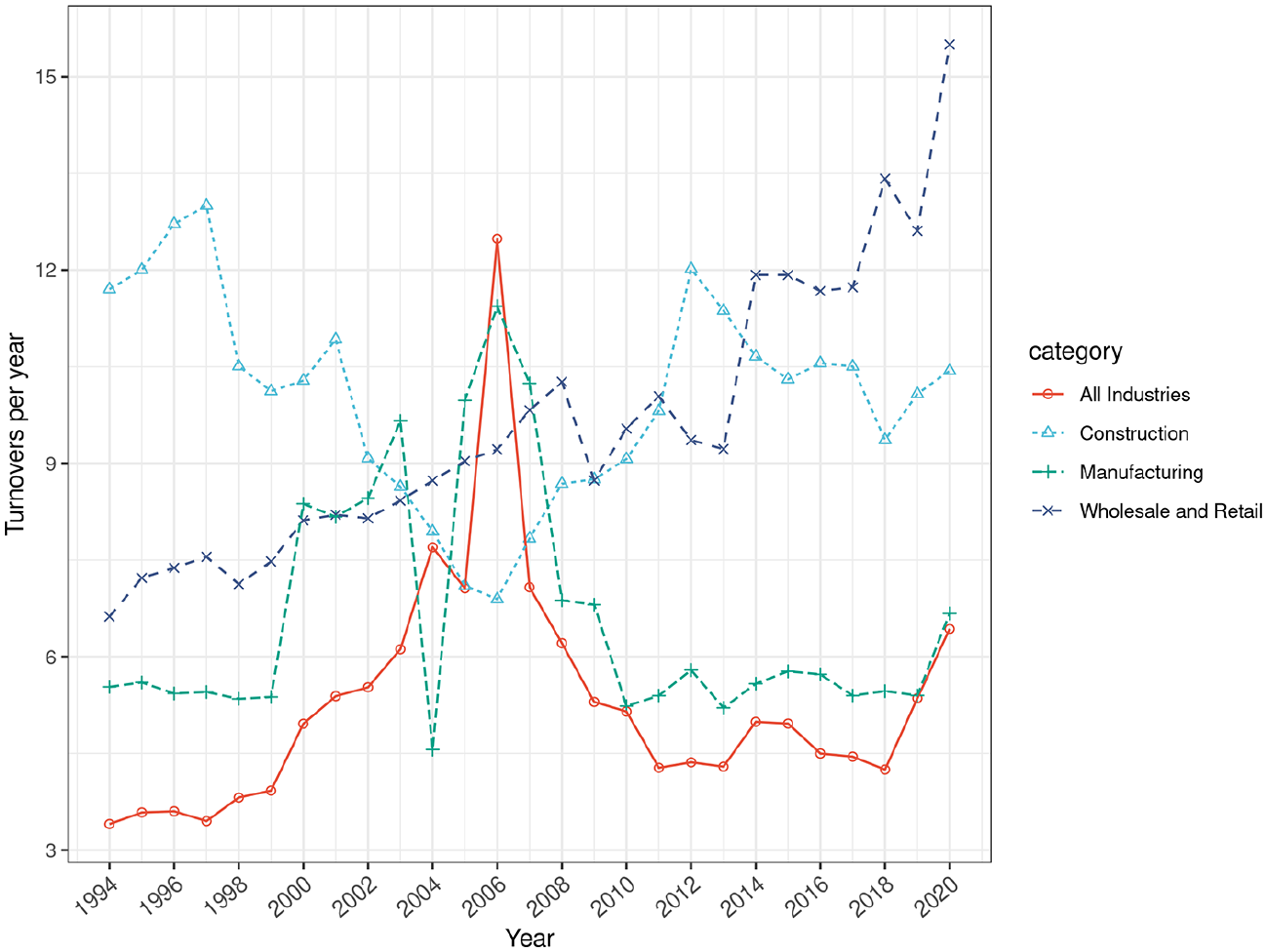
Sectoral turnover rates 1994–2020.

The widespread assumption that turnover is so fast as to render circulating capital a negligible quantity is unfounded for the whole economy. It ignores the fact that consumers, and particularly business consumers of intermediate products in business-to-business transactions, are reluctant to pay for their inputs even after having taken delivery of them; they attempt to lower their rate of turnover at the expense of their suppliers. This is particularly evident in wholesale and retail, where although turnover has risen across the period (presumably due to the application of computers, robots and direct Internet sales), monopsonies take deliveries of goods but only pay for them on, or after, sale. In construction, turnover slowed during the period of the housing boom when heightened demand meant building firms ran short of key materials and labour; while turnover rose in periods of lower housing demand, for the opposite reason. Mining (not included in this diagram for reasons of scale) shows the greatest fluctuation in turnover, with negative turnover rates in 12 of the years in this series counted as zero, alternating with years of very slow turnover such as 2011 with a rate of 2.5 during the post-crash recession; these variations exacerbate the enormous fluctuations in the profit rate peculiar to this sector.

The proportion of net fixed capital (DALD) in total capital advanced

In Figure 3, the proportion of fixed capital in total capital advanced indicates the technological and value composition of capital, which has slowly increased for all industries during this period, rising from 22% to 25%, albeit with fluctuations. Marx noted that rising productivity – the amount of use values produced per unit of value – cheapens the cost of reproduction of labour power and constant capital, thereby offsetting the tendency for the organic composition of capital to rise and so the rate of profit to fall. Trade with China and the US-China trade war after 2018 illustrate the impact of this tendency.

Figure 3.

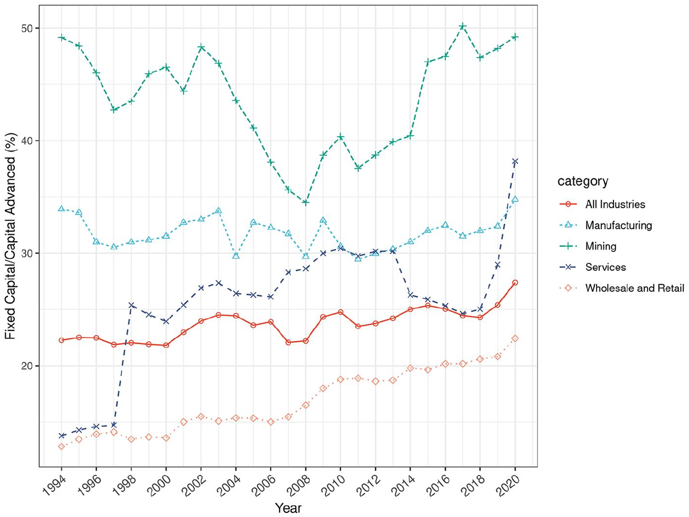
The net fixed capital/total capital advanced 1994–2020.

The US Bureau of Industry and Security (USBIS 2022) collated US-China trade statistics for 2021 of $2.8 trillion total U.S. Imports; $506.4 billion or 17.9% were from China, and of Chinese imports, 47.7% were machinery and mechanical appliances; 13.5%, furniture, bedding, lamps, toys, games, sport equipment, paint and 10.5%, other miscellaneous manufactured items (chemicals, plastics, rubber and leather goods). The value of US imports from China was $100 billion in 2000, $365 billion in 2010, $433 billion in 2020, and $537 billion in 2022 (United States Census Bureau (USCB) 2023). The price of consumer durables at 1982–1984 = 100, which peaked in 1996-1997 at 129.6 before steadily falling to 103.4 in 2020 and rising sharply to 128 in 2022 (FRED 2023). US imports from China from 2003 = 100 peaked in 2012 (105.5) and fell to 98 in 2020 and then rose to 104.5 in 2022 (U.S. Bureau of Labor Statistics (BLS) 2023b). This is in turn an effect of the trade war against China, as the price of Chinese imports has risen while substitutes are not yet available.

Large imports of Chinese products reduced the US cost of reproduction of labour power and thus lowered necessary labour and increased surplus value. This is reflected in the spending on food as a proportion of income, which steadily declined to around 9.4% by 2020, with an increasing part, roughly an equal share by then, spent away from home in takeouts and restaurants. After 2020, this fall went into reverse, rising albeit to a historically low level of 10.4% in 2021 (United States Department of Agriculture (USDA) 2022). The rise of services as a proportion of total output lowers the organic composition of capital, as services have a lower technical composition, a higher rate of turnover and are resistant to the replacement of labour with machinery.

The sectors with the largest proportion of fixed capital are mining and agriculture, which have very high technical composition of capital due to their dependency on machinery. In manufacturing, the growth of imports of machinery and inputs has reduced the proportion of fixed capital as rising productivity in the import of equipment and raw materials has offset the rise in the physical scale of production. Counter-intuitively, services have a higher proportion of DALD to total capital advanced than manufacturing, as their higher turnover means they do not have to advance capital for circulating productive capital.

Total capital advanced by sector

Figure 4 shows total capital advanced by sector. These figures are not adjusted for inflation, which varies by sector and type of output but was estimated to be around 72% from 1994 to 2020 (BLS 2023a). As services and transportation and warehousing have a negative rate of turnover, their capitalists do not have to advance wages for productive workers. Their wages are paid for by the workers themselves from the outset; hence, the amount of capital advanced underestimates the weight of these sectors within the economy. Agriculture and mining form a very small part of total capital advanced (the total appears to fall in 2020 only as figures for finance are unavailable for that year).

Figure 4.

The sectoral total capital advanced 1994–2020.

The largest sectors in 2020 were wholesale and retail, as well as services, which had far surpassed finance after the 2008 credit crunch. The total amount of capital advanced varies within a similar range to the BEA’s estimates of the Private Historic Net Fixed Capital Stock, their discounted aggregates of future profits, reflecting the existence of an average profit rate. Although the average absolute difference between them was 19.3% between 1994 and 2020, the impact on the rate of profit calculation was larger. The BEA’s measure is counter-cyclical and so tends to soften the peaks and troughs of the rate of profit. As an aggregate of discounted expected profits (not a measure of fixed capital advanced), it underestimates the total during periods of low profitability, thus overestimating the rate of profit, and overestimates during periods of high profitability, thus underestimating the rate of profit.

The impact of the growth in this trade on the US organic composition of capital is evident across all sectors and reflected in Figure 4: the proportion of fixed capital (or DALD) to total capital advanced (DALD/TCA).

The annual rate of surplus value

The annual rate of surplus value is the rate of surplus value multiplied by the rate of turnover;

it is equal to the rate of surplus-value produced by the advanced variable capital during one period of turnover, multiplied by the number of turnovers of the variable capital (which coincides with the number of turnovers of the entire circulating capital) (Marx 1956 [1885]: 181), with a further vital qualification.

In industrial capitalism, prices of production, not values, now form the centre around which prices fluctuate, such that the amount of surplus value realized in a sector bears no essential relationship to the amount of surplus value produced in it. Hence, the sectoral annual rate of surplus value includes transfers to and from (it is higher or lower than) the value annual rate of surplus value. In monopoly sectors with higher profits than the average or sectors with a higher-than-average value composition of capital, the workers there will appear to produce higher rates of surplus value than those in non-monopoly or lower organic composition sectors, who will appear to produce lower rates of surplus value. The financial sector appropriates profits from all productive sectors, and its revenues bear no direct relationship to production, even if the total interest is limited by the total amount of surplus value produced.

The calculation is further complicated because unproductive workers, including those who work in productive sectors, do not produce any surplus value at all; rather, they enable productive workers to produce it. Their wages are a direct cost to their employer, and since they have no direct product, they do not reduce turnover. As capitalists pay for unproductive circulating capital out of receipts, the proportion of these costs slows down the overall turnover. It is included in the estimate for the annual rate of surplus value to more accurately reflect the productivity of the collective labourer employed in a sector, bearing in mind that this sectoral annual rate of surplus value includes transfers, positive or negative, to and from other sectors. Total deduction is the aggregate of circulating capital, assuming that the proportion of unproductive and productive wages is the same as the proportion of COGS to TD (COGS/TD). Therefore, the formula for the annual rate of surplus value is:

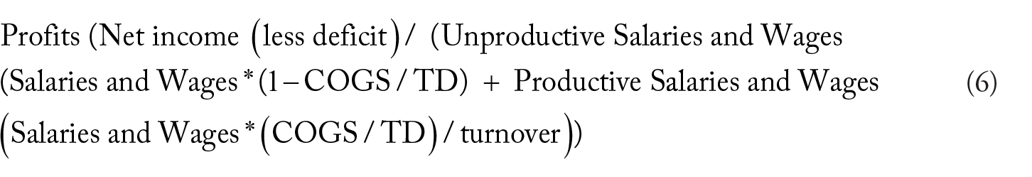
\begin{array}{l} Profits (Net income (less deficit) / (Unproductive Salaries and Wages \\ (Salaries and Wages * (1 - COGS / TD) + Productive Salaries and Wages \\ (Salaries and Wages * (COGS / TD) / turnover)) \end{array}

(6)

Figure 5 shows the sectoral annual rate of surplus value 1994–2020.

Figure 5.

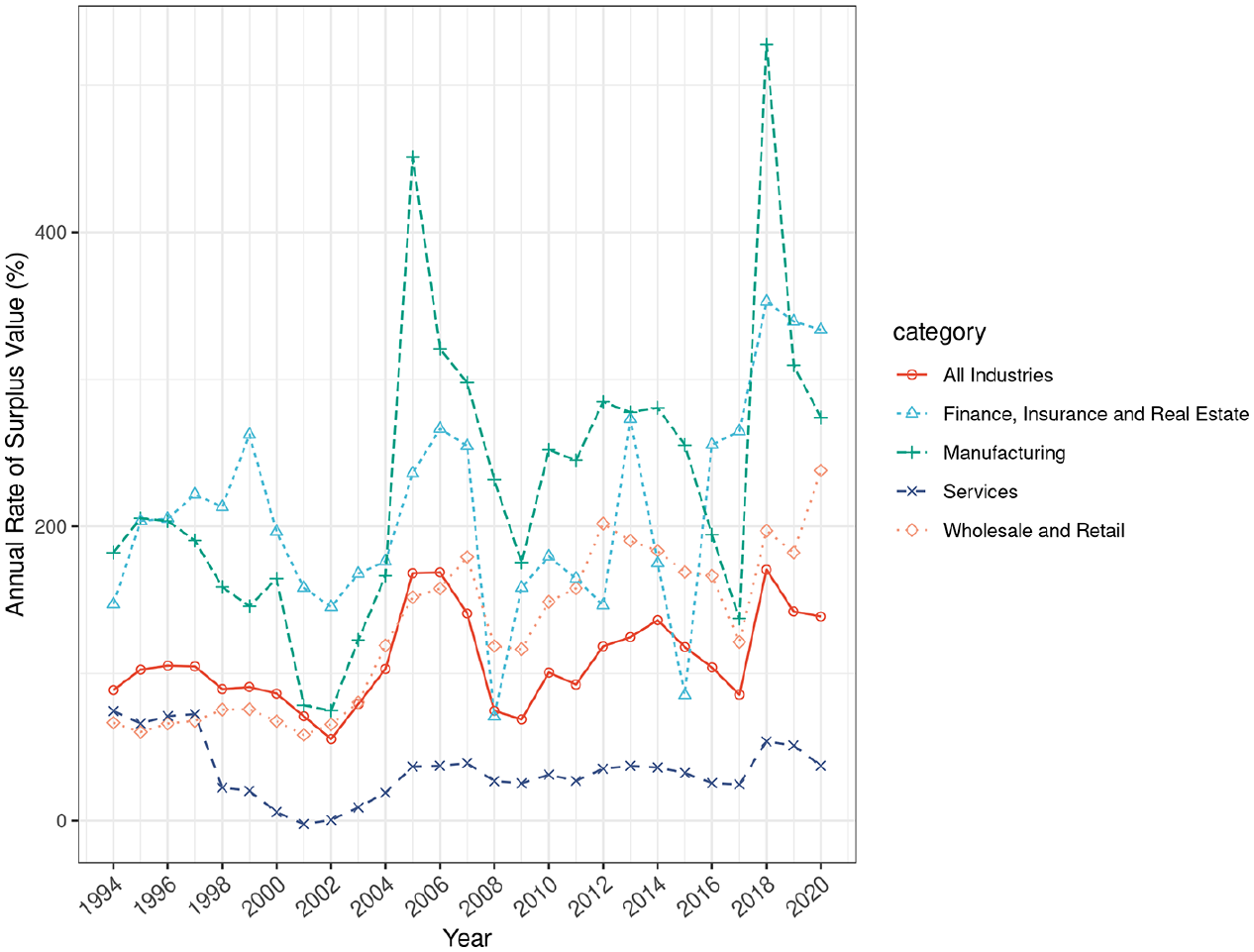
The sectoral annual rate of surplus value 1994–2020.

The transfer of value between sectors due to competition means these sectoral annual rates of surplus value could perhaps be more accurately described as the sectoral rate of profit commanded per wages advanced. It closely mirrors the sectoral enterprise rates of profit.

Enterprise rate of profit

Figure 6 shows the US Enterprise Rate of Profit for the main sectors of the US economy. Notwithstanding sharp differences in the technical composition of capital – due to the rate of turnover between sectors, the proportion of productive and unproductive labour and fixed and circulating capital, competition tends to establish an average cross-sectoral profit rate or price of production (barring mining and finance). Finance, which earns interest and not profits, and mining, which earns rents, are the two sectors which do not follow the general trend towards profit-rate equalization.

Figure 6.

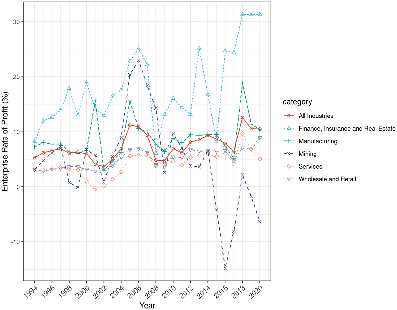
Sectoral enterprise rate or profit 1994–2020.

Mining is the most cyclical sector, while financial profit rates are probably particularly underestimated due to the offshoring of profits in tax havens, which are not declared in the USA. The repatriation of foreign profits may also explain some of the annual fluctuations in profit rates, such as for manufacturing in 2018. The growth of wholesale and retail reflects the vast profits made by US retail capitalists from unequal exchange. While the expansion of the Service sector is a consequence of the ongoing deflation of manufacturing goods and rising income inequality.

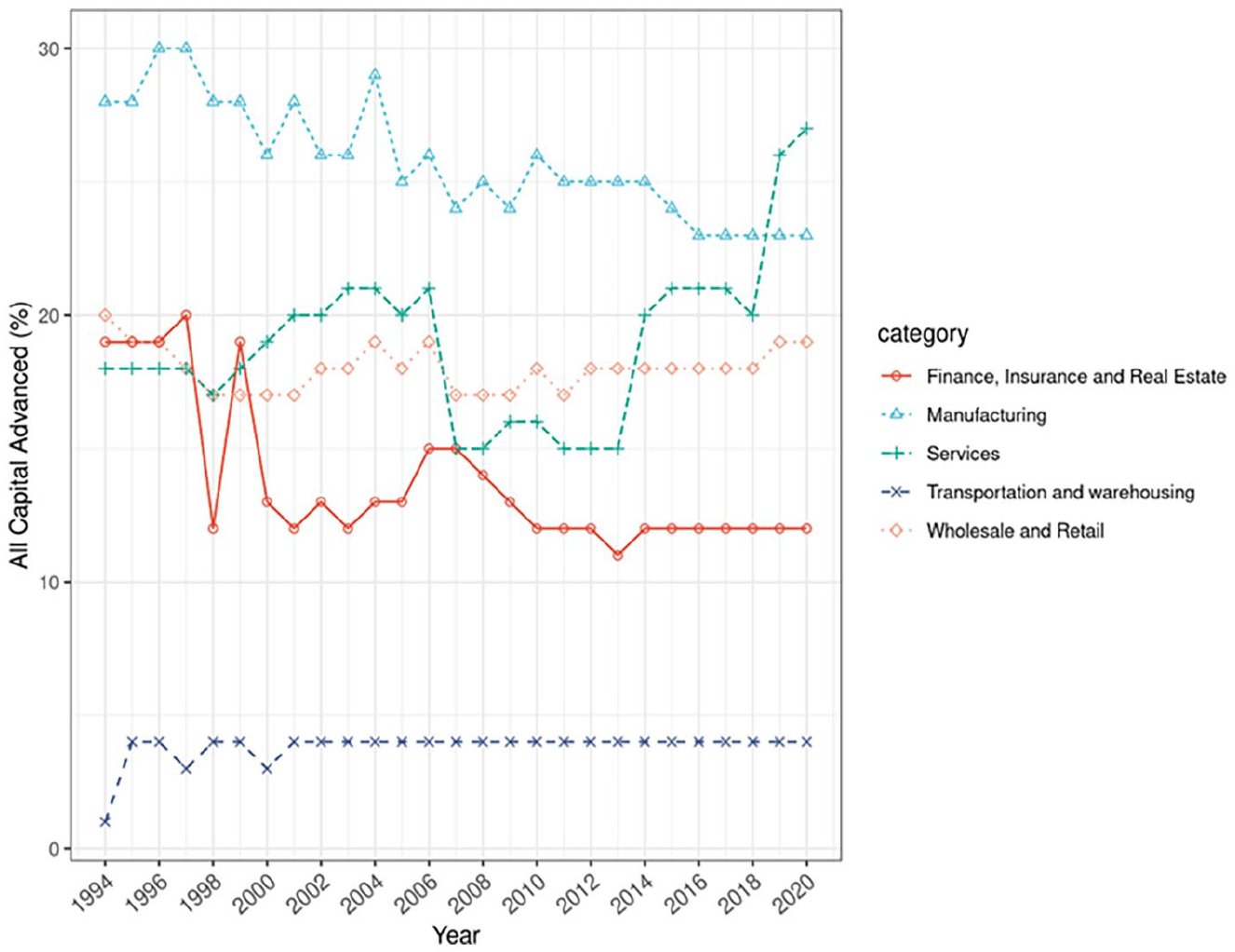
In Figure 7, average enterprise profit rates from 1994 to 2020 show the average weights of the sectors in total capital advanced and their average enterprise rates or profits across the period 1994–2020.

Figure 7.

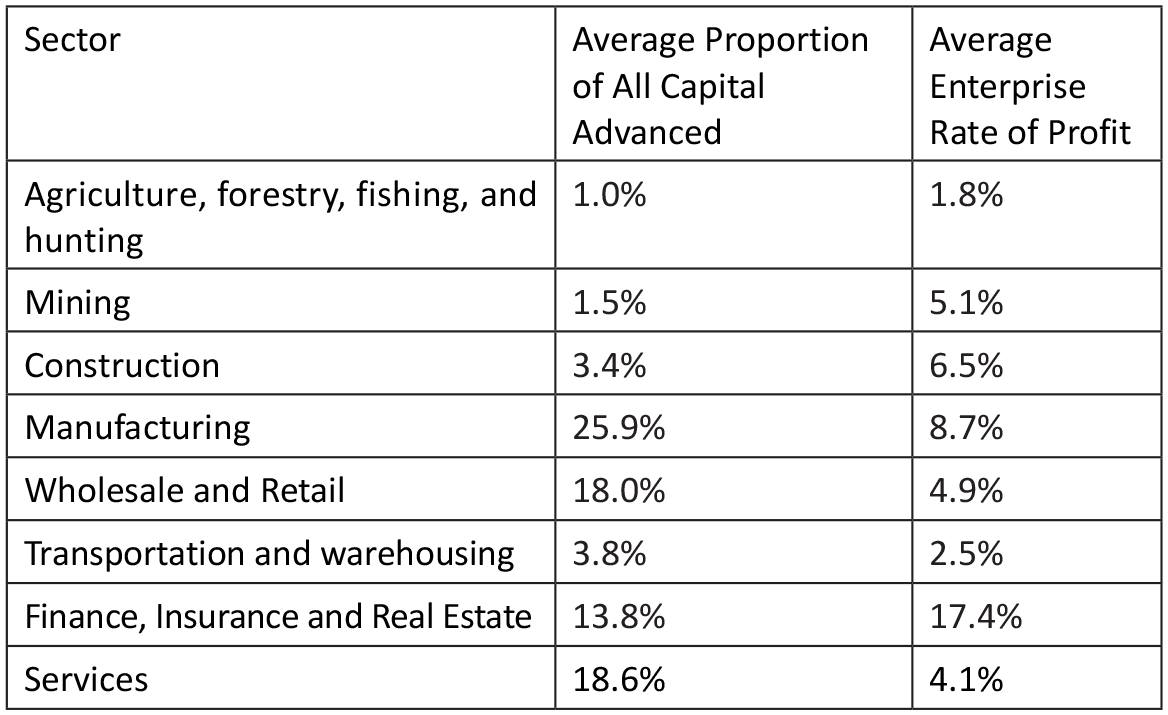
Average enterprise rate or profit 1994–2020.

The non-financial sectors (manufacturing, wholesale and retail, services, construction, transportation and warehousing and mining) show an average rate of profit range between 2.5% and 8.9%. Wholesale and retail and services accounting for on average around 37% of total capital advanced have an average enterprise rate of profit of 4.9% and 4.1%, respectively. Manufacturing, with a relatively lower turnover and thus higher proportion of total capital advanced (nearly 26%), has an average enterprise rate of profit of 8.7% (presumably due to monopoly power and a relatively higher organic composition of capital resulting in higher prices and so a higher profit rate). The only sector that stands far outside the standard range is finance, insurance and real estate, with a far higher average enterprise rate of profit of 17.4%.

Conclusion

Marx’s assumption of a tendency towards profit rate equalization, and the modification of values into prices of production that followed from it, was predicated on the existence of capitals with different value and organic compositions, rates of turnover and rates of surplus value. Such that the profit realized by a capitalist bore no essential relationship to the amount of surplus value produced by them. As all money is conceptually equal, and as capitalists expect all parts of their investment to yield the same profit rate, competition between capitals tends to establish an equal profit rate, such that the collective capitalist shares in the exploitation of the collective working class, driving capitalists together, even while competitive struggles drive them apart. The existence of this tendency is controversial within the Marxist political economy due to both conceptual and empirical shortcomings. The conceptual critique abandons any explanation of how competition modifies values into prices of production, while the empirical critique rests on Hulten and Wykoff’s neo-classical valuations of an ‘imaginary capital’ stock.

Hulten and Wykoff valuations of the FCS, as used in the UN SNA, are akin to the securitisation of ground rent, discounted aggregates of anticipated future benefits. They are specifically not estimates of fixed capital advanced (the cost of capital invested and so tied up in production). They are conceptually incoherent, insofar as any estimate of the rate of profit using them combines profits in the numerator and denominator of the calculation. They are practically incoherent, as Hulten and Wykoff valuations of the FCS would only equal costs if there were no profits, as they are explicitly not a measure of costs but an imputed ‘plausible’ estimate of future profits, not cost but opportunity cost. They are many times higher than actual quantities of value tied up in production and tend to even out fluctuations in profit rates. These valuations use the PIM and are specifically not limited to the initial year of installation. Even so, historic valuations of the FCS are lower than current ones, as income flows tend to decline in the years after the purchase of an asset. Furthermore, investment rates are explicitly adjusted to be consistent with the Hulten and Wykoff valuations of this imaginary capital. The equivalence of the individual and the aggregate is a fallacy of Hulten and Wykoff’s composition and is preserved and extended within the UN SNA (notwithstanding Joan Robinson’s acute criticism in the Cambridge Capital Controversy). The BEA’s overestimation of the value of the All-Industry FCS relative to the IRS is between 4 and 7 times, a pattern repeated in the sectoral data albeit with differences. The IRS DALD is a far more accurate estimate of actual capital accumulated in the FCS, as it measures actual assets installed by US capitalists after accumulated depreciation has been deducted.

Enterprise rate of profit includes interest and rent as a cost; it only applies at the level of the individual firm or sector. In aggregate, what is a cost for one is a revenue for the other; so costs, interest and rent can be disaggregated into wages, surplus value and the depreciation of fixed capital, as well as changes to inventory stocks.

An examination of the capital composition of the different sectors reveals that the increase in the technical composition of capital, which underpins the tendency for the organic composition to rise and the tendency of the rate of profit to fall, has been offset by globalization and, in particular, the rise in Chinese trade with the US. The outbreak of the US-China trade war in 2018 threatens to undermine these offsetting factors. The estimation of actual enterprise profit rates, undertaken here for the first time, reveals that, notwithstanding very different capital compositions, there is a tendency towards an average rate of profit or production price, common to all sectors, with profits of the major sectors ranging between 4% and 9%, barring finance. Profit rates are not equal between sectors but have a tendency towards equalization, hindered by limits on competition, monopolization and so on, except for the financial sector which does not earn the rate of profit but the rate of interest.

Footnotes

ORCID iD

William Jefferies

Author biography

William Jefferies has studied value theory and its application to globalization over the last years, including the misapplication of neoclassical statistics in his book 2015 book Measuring the Centrally Planned Economies and here in the estimation of the rate of profit, which is further developed in his 2025 book War and the World Economy.

References

Basu

Moraitis

(2023) Alternative approaches to labor values and prices of production: Theory and evidence. UMass Amherst Economics Working Paper Series 2023-4. Amherst, MA: UMass Amherst. Available at: https://scholarworks.umass.edu/econ_workingpaper/347/

Basu

Julio

Lara

, et al. (2025) World profit rates, 1960–2020. Review of Political Economy 37: 92–107.

Bjerkholt

(2016) Wassily Leontief and the discovery of the input-output approach. Memorandum, 18/2016. Oslo: Department of Economics, University of Oslo, p. 37.

Böhm-Bawerk

(1891) The Positive Theory of Capital (trans. Smart

). New York: G. E. Stechert.

Bureau of Economic Analysis (BEA), U.S. Department of Commerce (2003) Fixed Assets and Consumer Durables in the United States, 1925-97. Washington, DC: U.S. Government Printing Office.

Cockshott

Cottrell

(2003) A note on the organic composition of capital and profit rates. Cambridge Journal of Economics 27: 749–754.

Coen

(1978) Comment to on the feasibility of equating tax to economic depreciation. In: Hulten

Wykoff

(eds) Compendium of Tax Research Office of Tax Analysis. Washington, DC: Department of the Treasury, pp. 121–128. Available at: https://home.treasury.gov/system/files/131/Report-Compendium-1978-Part4.pdf

Fabricant

(1938) Capital Consumption and Adjustment. Cambridge, MA: National Bureau of Economic Research (NBER).

Farjoun

Machover

(1985) Probability, economics and the labour theory of value. New Left Review 1/152: 95–108.

10.

Farjoun

Machover

(2020) Laws of Chaos. London: Verso Books.

11.

Feenstra

Inklaar

Timmer

(2015) The next generation of the Penn World Table. American Economic Review 105(10): 3150–3182.

12.

Fraumeni

(2000) The measurement of depreciation in the US national income and product accounts (BEA). Joint Eurostat/OECD meeting on the national accounts, CES/AC.68/2000/W:1. Paris: OECD.

13.

FRED (St Louis Fed) (2023) Consumer price index for all urban consumers: Durables in U.S. city average (CUSR0000SAD). Available at: https://fred.stlouisfed.org/series/CUSR0000SAD

14.

Friedman

(1955) Review of Leon Walras and his economic system. The American Economic Review 45(5): 900–909.

15.

Hall

(1968, January) Technical change and capital from the point of view of the dual. Review of Economic Studies 35(1): 35–46.

16.

Hulten

Wykoff

(1978) On the feasibility of equating tax to economic depreciation. In: Hulten

Wykoff

(eds) Compendium of Tax Research Office of Tax Analysis. Washington, DC: Department of the Treasury, pp. 90–120. Available at: https://home.treasury.gov/system/files/131/Report-Compendium-1978-Part4.pdf

17.

Hulten

Wykoff

(1981a) The estimation of economic depreciation using vintage asset prices; An application of the Box-Cox power transformation. Journal of Econometrics 15: 367–396.

18.

Hulten

Wykoff

(1981b) The measurement of economic depreciation. In: Hulten

(ed.) Depreciation, Inflation, and the Taxation of Income from Capital. Washington, DC: The Urban Institute Press, pp. 81–125.

19.

Hotelling

(1925) A general mathematical theory of depreciation. Journal of the American Statistical Association 20(151): 340–353.

20.

Internal Revenue Service (IRS) (2005) 2005 corporation returns – explanation of terms. Available at: https://www.irs.gov/pub/irs-soi/05cosec5ccr.pdf

21.

Internal Revenue Service (IRS) (2022) SOI Bulletin historical Table 13. Available at: https://www.irs.gov/statistics/soi-tax-stats-historical-table-13

22.

Jefferies

(2021) Marx’s forgotten transformation solution: The transformation of values into prices of production in Marx’s Grundrisse and Maksakovsky’s the capitalist cycle. History of Economics Review 80(1): 18–37.

23.

Jefferies

(2023) The US rate of profit 1964–2017 and the turnover of fixed and circulating capital. Capital & Class 47(2): 267–291.

24.

Jefferies

(2024) The US enterprise rate of profit 1994-2020 statistical dataset. Available at: https://www.researchgate.net/publication/370215147_Enterprise_profit_rates_1994_to_2019

25.

Jorgenson

(1974) The economic theory of replacement and depreciation. In: Sellekaerts

(ed.) Econometrics and Economic Theory. London: Macmillan, pp. 189–223.

26.

Marquetti

Maldonado Filho

Lautert

(2010) The profit rate in Brazil, 1953-2003. Review of Radical Political Economics 42(4): 485–504.

27.

Marquetti

Miebach

Morrone

(2021) The Extended Penn World Tables 7.0. Texto para Discussão 2021/01. UFRGS.

28.

Marx

(1956 [1885]) Capital A Critique of Political Economy Volume II. Moscow: Progress Publishers.

29.

Marx

(1959 [1894]) Capital A Critique of Political Economy Volume III. Moscow: Progress Publishers.

30.

Marx

(1972 [1863]) Theories of Surplus Value Part 3. Moscow: Progress Publishers.

31.

Marx

(1973 [1857–1858]) Grundrisse (trans. Nicolaus

). London: Penguin Books.

32.

Michl

(2023) The falling rate of profit as a research program. The New School Economic Review 12: 36–51. Available at: https://nsereview.org/index.php/NSER/article/view/112

33.

OECD (2009) Measuring Capital Manual. 2nd ed. Paris: Organisation Economic Cooperation and Development (OECD).

34.

Roberts

(2020) A world rate of profit: A new approach. Available at: https://thenextrecession.wordpress.com/2020/07/25/a-world-rate-of-profit-a-new-approach

35.

Roberts

(2023) Is the US rate of profit been falling or rising? Available at: https://thenextrecession.files.wordpress.com/2023/01/reply-to-jefferies-030123.pdf

36.

Robinson

(1953) The production function and the theory of capital. Review of Economic Studies 21(2): 81–106.

37.

Shaikh

(2016) Capitalism; Conflict, Competition and Crises. Oxford: Oxford University Press.

38.

United Nations (UN) (2009) System of National Accounts. New York: United Nations.

39.

United States Bureau of Industry and Security (USBIS), U.S. Department of Commerce (2022) 2021 statistical analysis of U S trade with China, 29 April. Available at: https://www.bis.doc.gov/index.php/documents/technology-evaluation/ote-data-portal/country-analysis/2971-2021-statistical-analysis-of-u-s-trade-with-china

40.

United States Census Bureau (USCB) (2023) Trade in goods with China. Available at: https://www.census.gov/foreign-trade/balance/c5700.html

41.

United States Department of Agriculture (USDA) (2022) Total Food Budget Share Increased from 9.4 Percent of Disposable Income to 10.3 Percent in 2021. Washington, DC: USDA Research Department. Available at: https://www.ers.usda.gov/data-products/chart-gallery/gallery/chart-detail/?chartId=76967

42.

U.S. Bureau of Labor Statistics (BLS) (2023a) CPI inflation calculator. Available at: https://www.bls.gov/data/inflation_calculator.htm

43.

U.S. Bureau of Labor Statistics (BLS) (2023b) Import price index by origin (NAICS): All industries for China [CHNTOT]. Available at: https://fred.stlouisfed.org/series/CHNTOT

44.

Walras

(1954) Elements of Pure Economics, a Translation by W. Jaffé of the Edition Définitive (1926) of the Eléments d’économie pure, First Edition Published in 1874. Homewood, IL: Richard D. Irwin.

45.

World Input Output Database (WIOD) (2023) Groningen growth and development centre: Faculty of economics and business. Available at: https://www.rug.nl/ggdc/valuechain/wiod/?lang=en

46.

Zachariah

(2009) Determinants of the average profit rate and the trajectory of capitalist economies. Bulletin of Political Economy 3(1): 13–36.

The enterprise rate of profit in key US sectors 1994–2020: An examination of the tendency towards the equalization of sectoral profit rates and a critique of Hulten and Wykoff fixed capital stock valuations in the US

Abstract

Keywords

Introduction

Capital consumption, depreciation, and investment

Capital advanced the Internal Revenue Service alternative

How much do the SNA overvalue the FCS?

Enterprise rate of profit formula

The rate of turnover, ratio of fixed to circulating capital and productive and unproductive capital, the annual rate of surplus value and the equalization of the enterprise rate of profit

Sectoral turnovers and circulating capital advanced

The proportion of net fixed capital (DALD) in total capital advanced

Total capital advanced by sector

The annual rate of surplus value

Enterprise rate of profit

Conclusion

Footnotes

ORCID iD

Author biography

References