Sage Journals: Discover world-class research

Abstract

This article addresses how Marxist economists have estimated the quantity of fixed and circulating capital advanced in the denominator of the rate of profit calculation. Generally, Marxist economists have used neoclassical fixed capital estimates of opportunity cost, as applied most notably, in the US system of national accounts. These Hulten and Wyckoff measures aggregate the lifetime revenues (both costs and profits) of fixed assets and so grossly over estimate the value of the fixed capital stock. This article applies the Internal Revenue Service Depreciable Assets less Depreciation for a more accurate estimate of the actual quantity of fixed capital advanced. Furthermore, it criticises the absence of a convincing measure of the rate of turnover of Marx’s circuit of capital accumulation M . . . C . . . P . . . C’ . . . M’ in most rate of profit estimates. Developing the work of Bertrand and Fauqueur, this article demonstrates that the cash conversion cycle or net operating cycle mirrors Marx’s circuit. This article applies the cash conversion cycle to Internal Revenue Service Total Corporations data 1964–2017 to estimate the rate of turnover. The article addresses the distinction between unproductive and productive output and develops an estimation of those respective quantities based on Internal Revenue Service data. It combines these elements together to estimate the US rate of profit from 1964 to 2017. It finds that the US rate of profit rose strongly, albeit with dramatic fluctuations, after 2001.

Keywords

cash conversion cycle circulating capital fixed capital stock rate of profit turnover time

Introduction

The rate of profit calculation surplus value/constant and variable capital (s/c + v) critically depends on the amount of capital advanced or tied up in production. This in turn depends on the reproduction time of the components of capital. The cost of constant fixed capital (CFC) less depreciation or fixed capital advanced (FCA) and the cost of constant circulating and productive variable capital (CVC and PVC) are divided by turnover (T) and the stock of inventories (I). Capitalism is above all else a form of commodity production; products must be sold to realise the value incorporated in them during production. Unproductive activities, such as finance, insurance and retail, add no surplus value (S/V), but enable the realisation or sale of commodities. The cost of these activities is a transfer from the productive sector, and as they have no product, this unproductive cost (UC) does not turn over. Hence a fuller version of the rate of profit calculation could be S/(FCA + I + CCC/T + PVC/T + UC).

Marxist estimates of the profit rate have only haphazardly addressed the turnover rate of circulating capital. This appears to be for several reasons. They typically use neoclassical valuations of the fixed capital stock that aggregate its income streams, including profits, and so grossly overvalue its cost. This overvaluation is so disproportionately large that the amount of circulating capital makes little difference to the profit rate calculation; furthermore, the rate of turnover is assumed to be so high that once the already disproportionately small proportion of circulating capital advanced has been deflated by it, it becomes vanishingly tiny and immaterial; and finally, there does not appear to be an obvious way to work out turnover. Theorists have looked at inventories and sales, and their ratio, but these attempts have been flawed, not entirely consistent with Marx’s definition and lacking empirical evidence. This article attempts to provide answers to these problems.

The fixed capital stock and their neoclassical valuation

The amount of fixed capital advanced consists of the gross capital replacement cost (either at historic (purchase price) or current (replacement price)) multiplied by a discard function, the rate of depreciation. This is, in its turn, dependent on the asset lives used. The total value of fixed capital is completely reproduced, that is, fully returned to circulation, only when it has been completely consumed in the production process. Fixed capital re-enters circulation according to its initial amount and the rate of its wearing out or the period of its obsolescence. Marx (1978 [1885]) noted that ‘the longer an instrument lasts, the slower it wears out, the longer will its constant capital-value remains fixed in this use-form’; he continued, ‘if of two machines of equal value one wears out in five years and the other in ten, then the first yields twice as much value in the same time as the second’ (p. 93). After the machine is fully depreciated the machine no longer adds value to the asset. Rather, any income it yields consists of new value created by the workers who use it and transfers of value from other capitalists who do not own the same machine. By manipulating rates of depreciation, capitalists may foreshorten the rate of depreciation and so recover the assets value more quickly than the duration of its service life (Marx 1978 [1885]: 104). Higher rates of depreciation reduce the absolute rate of profit in the short run, but then increase it faster, all things being equal, as the reduction in S/V is repetitive, but the reduction in capital advanced is cumulative. Once the investment has been fully depreciated, the transfer of value to the capitalist owner of the machine from the capitalists who do not own the machine is only reduced by maintenance costs for the remaining service life of the machine.

Soloman Fabricant (1938) developed the neoclassical method underpinning the valuations of the US Bureau of Economic Analysis (BEA) today. Fabricant’s valuation of fixed capital is a multiple of the expected revenues the fixed capital yields. It is necessarily higher than the actual purchase price or replacement cost of the capital, except in the imaginary world of perfect competition where there are no profits and so the notional revenues generated by the asset equal costs (Fabricant 1938: 8–9). As the fixed capital ages, so these revenues decline. Economists’ depreciation measures the rate of decline of income generated by a new asset over its service life or the period in which the asset produces revenues (Bureau Economic Analysis (BEA) 2003: 5). It is a measure of the change of opportunity cost (Hulten & Wykoff 1981: 86). Economists’ depreciation historic cost is a multiple of the (above purchase price) revenues that the asset created on installation, while economists’ depreciation current cost is a multiple of the (above replacement price) revenues that the asset would create on replacement. This is far longer than the period in which actual installation or replacement costs are recovered. Consequently, these neoclassical depreciation rates are substantially lower than the actual taxation depreciation rates, which cover the period in which the installation cost of the asset is recovered (Hulten & Wykoff 1981: 91). Irrespective of the depreciation period, the actual cost of the fixed capital stock, the actual amount of fixed capital advanced (whether historic or current) plays no part in the neoclassical valuations of the fixed capital stock applied in the system of national accounts (SNA).

The Bureau of Economic Analysis (BEA) applies Fabricant’s method to schedules developed by Charles Hulten and Frank Wykoff (1981). The BEA’s (2003) ‘real cost’ or ‘market cost’ or the so-called ‘net present value’ of an asset equals the discounted sum of its future income stream, the amount of interest or revenue it yields minus costs accumulated over the service life of the asset (p. 2). It is not its real cost or market cost or net present value. To calculate the current or historical net fixed capital stock at the end of year the revenues the asset produces are summed over all vintages of investment flows for that asset (BEA 2003: 7). If, for example, a new machine cost 100, has a service life of 5 years and after deducting costs, raises profits by 100 each year (consisting of new S/V added and transfers from other capitalists), then the actual rate of profit is 100/100 or 100%. However, the BEA would value the machine at 500, the aggregate of profits it generates, and so the rate of profit in the national accounts would be 100/500 or 20%. Paradoxically, as profits rise, so the valuation of the fixed capital stock does too, so the profit rate falls or rises more slowly than it should, depending on the relative proportions of the numerator and denominator of the rate of profit calculation. Measures of the productive capital stock are adjusted for ‘economic decay rather than for losses of value due to economic depreciation’ (Mohr & Gilbert 1996: 2). The Organisation for Economic Co-operation and Development (OECD, 2009) emphasises that the SNA explicitly asserts that

Unlike depreciation as usually calculated in business accounts, consumption of fixed capital is not, at least in principle, a method of allocating the costs of past expenditures on fixed assets over subsequent accounting periods’. In other words, depreciation is a forward-looking measure that is determined by future, not past, events. (p. 52)

The neoclassical valuations of the fixed capital stock rest on the tautology so effectively criticised by Joan Robinson (1953) during the Cambridge Capital Controversy. Robinson (1953) explained that profits appeared as a cost of production ‘the Profit on that part of the cost of capital represented by this profit is then a component of the ‘cost of production of final output’’ (p. 88), so that ‘the value of an equipment depends upon its expected future earnings. It may be regarded as future earnings discounted back to the present at a rate corresponding to the ruling rate of interest’ (Robinson 1953: 89). The value of capital depends on the rate of interest and the rate of interest depends on the value of capital. The higher the rate of interest, the more valuable the capital, and the lower the rate of interest, the less valuable the capital, so that conceptually the rate of return never changes. Although as the SNA’s valuations of the fixed capital stock and rates of depreciation are given by the Hulten and Wykoff schedule, there is some movement, usually downwards, as rising profits appear as increased costs. The fundamental point is that the SNA’s valuations of fixed capital, and so economists’ depreciation, does not correspond at all to the amount of capital advanced for fixed capital, as it includes profit in both the numerator and the denominator of the rate of profit calculation.

Accountants’ Depreciation, however, measures the amount of capital tied up in the fixed capital stock. The Internal Revenue Service (IRS) uses the modified accelerated cost recovery system (MACRS) to specify the service lives and methods for the depreciation of tangible property according to the class of asset or business. This information is very accurate as depreciation is 100% tax deductible, so firms have a very strong incentive to report investments as the cost of investment is borne by the collective capitalist. The general depreciation system (GDS) is the most common method used, while the alternate depreciation system (ADS) is generally limited to property which is not solely used for business purposes, such as small traders using their vans for domestic work and use IRS (2018). The ADS allows a longer service life and so a slower rate of depreciation (DOT 2000). The general rule for Accountants’ Depreciation is 200% declining-balance (200%DB). The MACRS system applies the 200%DB rule and is the standard category used by US corporations. Divide the asset cost price by the expected period of depreciation and then multiply by two. Assets are divided into classes according to the period in which they are depreciated, but the 200%DB rule ensures that depreciation is frontloaded.

The IRS (1964–2017) labels the historic cost or purchase price of fixed capital as Depreciable Assets. Accumulated Depreciation is the sum of all recorded depreciation on an asset to a specific date. Depreciable Assets less Accumulated Depreciation is the assets’ Carry Value, or the current amount of capital advanced for the asset. Carry Value differs very significantly from the estimates of the value of the fixed capital stock, used by the BEA. The IRS measure of Carry Value is around 22% of the BEA historic cost fixed capital stock measure between 1964 and 2017. IRS (1987) Rev. Proc. 87-56 gives the service lives for Accountants’ Depreciation in the United States. The asset class lives of IRS and Hulten and Wykoff categories are not directly comparable, so the selection in Table 1 features those categories which are particularly closely aligned. Table 1 contrasts the BEA Hulten and Wykoff measures with IRS GDS and ADS service lives for selected categories.

Table 1.

Hulten and Wykoff service lives and GDS and ADS service lives.

OECD Hulten & Wykoff (H&W) class name	Machinery and equipment service life years	IRS class name	Class Life Years	GDS (MACRS)	ADS	GDS (MACRS)/H&W
Manufacture of food products, beverages, tobacco	27	Manufacture of Tobacco and Tobacco Products. Asset class 21	15	7	15	26%
Manufacture of textile and leather products	35	Manufacture of Yarn, Thread, and Woven Fabric Asset class 22	11	7	11	20%
Manufacture of wood and products of wood	30	Manufacture of Wood Products, and Furniture Asset class 24.4	13	7	13	23%
Manufacture of chemicals, chemical products	30	Manufacture of Chemicals and Allied Products Asset class 28	9.5	5	9.5	17%
Manufacture of rubber and plastic products	30	Manufacture of Rubber Products Asset class 30.1	14	7	14	23%
Manufacture of fabricated metal products	33	Manufacture of Fabricated Metal Products Asset class 34	12	7	12	21%
Manufacture of machinery and equipment n.e.c.	33	Manufacture of Electrical and Non-Electrical Machinery and Other Mechanical Products Asset class 35	10	7	10	21%
Manufacture of office machinery and computers	21	Manufacture of Electronic Components, Products, and Systems Asset class 36	6	5	6	24%

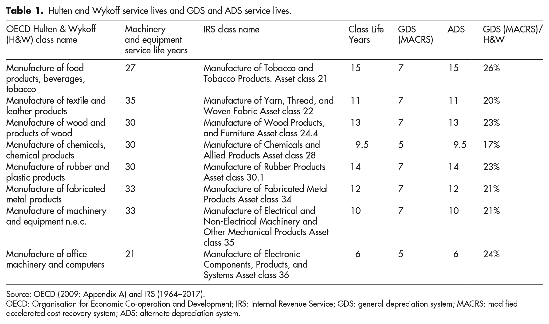
Source: OECD (2009: Appendix A) and IRS (1964–2017).

OECD: Organisation for Economic Co-operation and Development; IRS: Internal Revenue Service; GDS: general depreciation system; MACRS: modified accelerated cost recovery system; ADS: alternate depreciation system.

On average the BEA figures overestimate the depreciation period by 460% or GDS (MACRS)/H&W is around 22%, which confirms the proportion of the IRS Depreciable Assets Less Depreciation to the BEA historic fixed capital stock referred to above (Jefferies, 2021).

Marxist political economy has not considered the key distinction between economists’ and accountants’ depreciation, but rather debated whether fixed capital valuations should be based on the BEA’s neoclassical historic or current cost fixed capital stock valuations (Basu & Vasudevan 2013: 63). Marxian economists are apparently unaware of the significance of the distinction between costs and opportunity costs. For, as profits rise in the numerator so they rise in the denominator to the same amount but in the opposite direction. By including profits or interest in both the numerator and the denominator of the rate of profit calculation, so an increase in profits is measured as a fall of it, as in Roberts and Carchedi (2018) and Tsoulfidis and Tsaliki (2019).

Circulating capital

The categorically mistaken use of neoclassical opportunity cost measures of the fixed capital stock is compounded by the assumption, without any empirical justification, that the turnover time is so fast that the cost of circulating capital is essentially negligible (Tsoulfidis & Tsaliki 2019). This implies that circulating, including variable, capital can be ignored in estimates of profit rates (Kuczynski, 1992: 266). This assumption fails to account for; first, the significant lags between delivery and payment for intermediate inputs, including energy, raw materials, semifinished goods and services (both produced by, and purchased from domestic industries and foreign sources) that an industry consumes in producing its gross output (GO; Strassner et al. 2005: 34). Second, that only productive labour, labour that produces a product which is sold on the market turns over at all. Unproductive labour does not turn over as it has no product, it adds no value but is still a cost for capitalists who must sell their output to realise the value in it. Even in productive sectors like manufacturing a large proportion of wage expenses are on unproductive labourers, administration, human resources, research and development or management. Retail is a combination of unproductive and productive activities such as shipping and assembly (productive) and warehousing and sales (unproductive), while Finance and Insurance have no product and so no turnover. To complicate the picture further, all sectors in the United States realise significant quantities of value produced abroad but credited to domestic production through unequal exchange. This makes it difficult to separate out the different activities according to a strict interpretation of Marx’s categories. To be consistent with the data the unproductive sectors referred to in the calculation of the rate of profit here are those as defined by the IRS through the proportion of cost of goods sold (COGS) to total deductions (TD) (COGS/TD).

The phases of the turnover of circulating capital and the cash conversion cycle or net operating cycle

Following Marx and Engels it is assumed here that the turnover of productive variable capital, or wages, is the same as the turnover of circulating capital. Engels noted that that the ‘only essential distinction’ which capital impresses upon the capitalist is ‘that of fixed and circulating capital’ (Marx 1966 [1894]: 48). These components of productive capital have ‘the parts of its value invested in labour-power and in means of production which do not constitute fixed capital – by reason of their common turnover characteristics confront the fixed capital as circulating or fluent capital’ (Marx’s emphasis, Marx 1978 [1885]: 97). The value of the circulating capital – in labour-power and means of production – is advanced only for the time during which the product is in the process of production. This value enters entirely into the product, is therefore fully returned by its sale from the sphere of circulation and can be advanced anew (Marx 1978 [1885]: 98). This value circulates with the product containing it. The product assumes the form of money through the sale of the product and must then, to ensure the continuity of the production process, be reconverted into the same elements of production as were used up in producing it. Labour is paid for (usually weekly or monthly) separately from raw materials or other intermediate products, as new and old value added is combined in the product, the reconversion ‘into money of the part of capital laid out in labour-power goes hand in hand with that of the capital invested in raw and auxiliary materials’ (Marx 1978 [1885]: 112). The rate of turnover of variable capital depends on the rate of reconversion of the products in which the value of labour is embodied; Marx (1978 [1885]) observed:

capital of a given magnitude is simultaneously, though in varying proportions, divided, within this flow and succession of forms, into different forms: productive capital, money-capital, and commodity-capital, so that they not only alternate with one another, but different portions of the total capital-value are constantly side by side and function in these different states. (p. 215)

Production and circulation periods only add to turnover time to the extent that they tie up capital or extend total turnover. If production takes 10 days and circulation takes 10 days, if the periods are consecutive then their sum is 20 days, but if, for example, a part of circulation, say 8 days, occurs concurrently with production, such as marketing, finding a buyer for the product and selling it, then the sum of production and circulation times is 12 days, with only 2 days of circulation added to the sum that makes up total turnover time:

The duration of this turnover is determined by the sum of its time of production and its time of circulation. This time total constitutes the time of turnover of the capital. It measures the interval of time between one circuit period of the entire capital-value and the next, the periodicity in the process of life of capital or, if you like, the time of the renewal, the repetition, of the process of self-expansion, or production, of one and the same capital-value. (Marx 1978 [1885]: 91)

Circulating capital is physically incorporated into a product or used up during the production process as its value is incorporated into the product. This value is reproduced only when the product is sold (Marx 1978 [1885]: 369). Hugues Bertrand and Alain Fauqueur (1978) consider that circulating capital takes the form of three conceptually successive, although simultaneous, and overlapping, forms:

The hire of labour and purchase (or order of inputs to be paid for) intermediate goods or inventory of inputs;

The activity of production, wherein the labour force transforms the intermediate goods into products – to be delivered or to form stocks of finished products;

The realisation (sale) of stock or inventory as output, transforms this product into money which forms the funds for the next cycle of production, the purchase of intermediate goods and the re-employment (or hiring) of workers (Bertrand & Fauqueur 1978).

The multifaceted circulating fraction of capital simultaneously takes on multiple forms: productive capital (intermediate inputs or constant circulating capital and labour power), commodity capital (goods in stock, or in the process of production, or awaiting realisation) and money capital (awaiting to be reused to start a new cycle) (Bertrand & Fauqueur 1978). While conceptually production is continuous, a flow, the purchase of inputs and their sale as outputs is not. It is broken down into discrete inventory periods, a stock, in which inputs are purchased, stored in inventory, removed from inventory, productively consumed, transformed into outputs, returned to inventory, sold, shipped out of inventory, and paid for. These movements into and out of inventory provide a mechanism for measuring the average turnover of capital advanced for fluid or circulating capital in which turnover consists of purchase, payment, production, sale and realisation or the period it takes for M. . .M’. As Engels observed in Capital III:

owing to the time span required for turnover, not all the capital can be employed all at once in production; some of the capital always lies idle, either in the form of money-capital, of raw material supplies, of finished but still unsold commodity-capital, or of outstanding claims. (Engels in Marx 1966 [1894]: 46)

Verlyn Richards and Eugene Laughlin (1980) explained that ‘inventory turnovers depict the frequency with which firms convert their cumulative stock of raw material, work-in-process, and finished goods into product sales’ (Richards & Laughlin 1980: 33). They continued the ‘the cumulative days per turnover for accounts receivable and inventory investments approximates the length of a firm’s operating cycle’ (Richards & Laughlin 1980: 34). Capitalist production, as generalised commodity production, produces output which must be sold. Turnover cannot be faster than the lags caused by payment. The productive cycle begins when inputs are purchased and delivered, but often before they are paid for. Hence the cash conversion cycle (CCC) reflects:

the net time interval between actual cash expenditures on a firm’s purchase of productive resources and the ultimate recovery of cash receipts from product sales, establishes the period of time required to convert a dollar of cash disbursements back into a dollar of cash inflow from a firm’s regular course of operations. (Richards & Laughlin 1980: 34)

The longer the duration of turnover, the more capital is necessary in advance (for the wage fund and to purchase intermediate goods) and vice versa. The formulas can be found in Statistical Appendix 1.

The conceptually linear series M . . . C . . . P . . . C’ . . . M’ assumes that inputs are paid for before they are used, but this is very far from being the case. It should be emphasised that the chronological stages need not occur in the specified order, within the limits of the production process itself. Product may be paid for before it is delivered, it may be delivered before it is paid for, but it may not be delivered before it is produced. Just-in-time production may mean that stocks are delivered when they are used up, but whether they will be paid for is a different matter. Every capitalist seeks to reduce the time between delivery and payment for their outputs or accounts receivable, while simultaneously increasing the time between delivery, and payment for their inputs or accounts payable. As a result, intermediate, Business to Business (B2B) transactions have the slowest rate of turnover, due to the reluctance of capitalists to pay for their inputs and the necessity to have supplies of products available to meet fluctuations in demand. Output is not generally made to order or instantaneously sold. Capitalists seek to receive payments for the commodities they produce as quickly as possible, but to pay for commodities they receive as late as possible. This period is the difference between accounts receivable and accounts payable. According to the UK Office of National Statistics, on average firms take 37 days to pay invoices (Office for National Statistics (ONS) 2017). Atradius found that in 2018, of the 41.3% of the US firms provided with credit in Business-to-Business (B2B) transactions 50% of invoices were overdue. The average days sales outstanding (DSO) figure recorded in the Americas was 37 days while average payment times in the United States was 32 days (Atradius 2018). The average payment periods are broadly comparable, although they fluctuate according to the business cycle, and indicate the absolute limit on turnover rates determined by lags in payments for sales.

The number of times variable capital turns over in a year multiplies the rate of S/V by the number of turnovers to form the annual rate of S/V. The ratio of the total S/V annually produced to the value of the variable capital advanced (Marx 1978 [1885]: 371). Engels noted that the quantity of S/V is increased by reductions in the period of turnover or:

of one of its two sections, in the time of production and the time of circulation. But since the rate of profit only expresses the relation of the produced quantity of surplus-value to the total capital employed in its production, it is evident that any such reduction increases the rate of profit. (Engels in Marx 1966: 167)

The turnover time modifies ‘the size of the money capital that has to be advanced to set in motion a definite amount of labour-power in the course of the year’ (Marx 1978 [1885]: 387), so that ‘the velocity of turnover therefore – the remaining conditions of production being held constant – substitutes for the volume of capital’ (Marx 1973: 443). The faster the turnover, the more S/V can be extracted for the given quantity of capital advanced, and so the higher the rate of profit; necessarily then there is a ‘statistically significant relationship between the cash conversion cycle and profitability, measured through gross operating profit’ (Gill et al. 2010: 1).

GO and gross value added

The rate of turnover is a measure of the rate at which sales return money originally advanced back to the capitalist, this is distinct from, and separate to, value added. Marx (1973) observed that ‘the value which capital posits in one cycle, one revolution, one turnover, is = to the value posited in the production process, i.e. = to the value reproduced + the new value’ (Marx’s emphasis, p. 546). The typical assumption of one annual turnover generally used in Capital is arbitrary. Total value added and S/V as

the sum of values (surplus values) is thus determined by the value posited in one turnover multiplied by the number of turnovers in a given period. One turnover of capital is = to the production time + the circulation time. (Marx 1973: 550)

Capital, in its reality, therefore ‘appears as a series of turnovers in a given period’ (Marx’s emphasis, Marx 1973: 562). Leontief noted that in the turnover of the economy, this distinction needs to be emphasised. Sales include value that endlessly reappears as intermediate goods or costs:

This latter value is usually called costs. In statistical methodology, the definite distinction between these two value sums means that the first of these sums – the net product – can appear no more than once in the process of production. Cost expenditures, on the contrary, can endlessly pass from one stage of production to another and reappear at each stage in the same form. Thus, the net product of several branches of production is always equal to the sum of the individual net products; costs, on the contrary, amount to less than the sum of the individual total products since they constitute only a part of the total value of production and since the same values are accounted against and again in various technically related processes of production. (Leontief cited in Spulber 1964: 90)

Each turnover only adds a certain proportion of value added, so the rate of turnover is a rate of sale, and so is different to, and distinct from, the creation of value added. Thus, the total value added will constitute the proportion of value added in each sale multiplied by the number of sales or turnovers (Leontief cited in Spulber 1964: 93). The annual rate of profit for the entire economy includes aggregates of profits and wages in gross value added (GVA) rather than GO. The turnover rate shows how many times GO turned over in producing GVA. Hence circulating constant capital advanced (CCCA) or intermediate costs/turnover (IC/T) does not appear as a separate variable, rather productive variable capital divided by turnover (PVC/T) reveals the cost of circulating capital advanced in GVA.

The presence of these unsold and so unproductive services originates with Leontief’s complaint about the original Soviet Balance of 1923–1924. Based on an application of the schemes of reproduction in Capital II the Balance deemed government services to be unproductive. The Balance was limited to measures of the sales of physical use values in the Soviet New Economic Policy (NEP) 1921–1928 period. Leontief objected to this exclusion even though he conceded ‘the state does not create any material goods; its income is “derived” and as such does not have any counterpart in the income of the economic balance’ (Leontief cited in Spulber 1964: 89). When Leontief worked with Kuznets in developing the US SNA in the early 1930s, he ensured that unproductive government output was included in national income statistics.

Fred Moseley’s (1985, 1986) articles limited his estimates of the rate of S/V to the productive sectors of the economy. Productive sectors are those that produce a commodity for sale, excluding not only government output, but sectors involved in the circulation of commodities. Moseley (1986) explicitly bases this approach on the circuit of capital accumulation and differentiates between productive and unproductive variable capital, but does not estimate turnover (p. 173). The absence of turnover means that Moseley does not differentiate between the rate of S/V and the annual rate of S/V, the rate of S/V deflated by turnover. The restriction of rates of S/V to productive sectors is conceptually moot given that unproductive workers may be unnecessary to production, insofar as they produce no commodity, but they are of ‘central importance’ to the capitalist mode of production (Paitaridis & Tsoulfidis, 2018: 215). Both rates of S/V, including and excluding productive and unproductive sectors, reveal something about the workings of capitalism.

The IRS’ Total Corporation Data does not include government production IRS (2005). The COGS measures the amount of spending on intermediate inputs or circulating capital, while the cost of labour (COL) measures the cost of wages in COGS. IRS changed from cost of sales and operations (CSO), which is a broader category that includes administration and managerial costs, to COGS in 1994 (IRS 1964–2017). COGS separate the COL necessary for the manufacture of the product, from other labour costs, administration, sales etc. supervision and executive salaries. While the Finance and Insurance sector that produces no goods for sale, have no COGS (IRS 1964–2017: 298). As capital only exists in this mystified form, this article considers that the proportion of COGS to TD (COGS/TD) in the IRS data approximates the proportion of unproductive in final output.

Circulation time and the rate of profit discussed

Tom Weisskopf (1979) discussed various Marxian estimates of profit rates but determined to use one that did not include circulating constant capital other than in the form of inventory stocks, (corporate profits + net income)/ (fixed capital stock + inventories) (p. 349). Weisskopf (1979) used US Commerce Departments economists’ depreciation estimates of the fixed capital stock (p. 376). He developed the distinction between manufacturing workers directly employed in production, and salaried employees who do not, but he did not relate this to turnover, which he did not estimate (Weisskopf 1979: 355).

Edward Ochoa (1984) in his discussion of labour values and prices of production, observed that the circulating capital advanced as a stock of input materials and wage fund, should be deflated by a turnover-time vector t. This is ‘approximated by the sectoral inventory-sales ratios for 1963, the only year available’ (Ochoa 1984: 82). This is the proportion of inventory to value added not the rate of turnover. Ochoa did not calculate the annual rate of S/V separate from the rate of S/V. Ochoa’s (1989) article Values, Prices and Wage Profit Curves in the US Economy was based on sections of this PhD and claimed that ‘the level of material inventories and wages fund is related to their flows by the turnover time of circulating capital’, such that the ‘necessary stocks are simply (annual flows x turnover time). This would give us the stock levels necessary to produce one year’s output’ (Ochoa 1989: 416). As this calculation does not include the cost of goods or intermediate costs, it excludes circulating constant capital. As it assumes a constant rate of S/V, its value added is wages plus this assumed amount; all it shows is the proportion of inventories to this assumed value added. It does not tell us how many times that inventory has turned over to produce that value added.

Michael Webber and David Rigby’s (1986) discussion of the rate of profit in Canadian manufacturing noted that both circulating variable capital and constant capital needed to be deflated by turnover (p. 38). They emphasised that circulating capital is no trivial part of capital advanced, but significantly changes profit rates calculations (Webber & Rigby 1986: 43). Webber and Rigby assumed that inventories are divided between constant and variable capital in the same proportions as constant and variable capital in total costs. This assumption is not substantiated by the empirical evidence; the COL measures the proportion of that spending on the wages of productive labour; between 1994 and 2017 COL averaged around 9% of COGS (Authors calcs, IRS 1964-2017). As the total costs are the sum of circulating and constant costs, the deducting constant costs from total costs reveals circulating costs. If the proportion of circulating costs in total costs is multiplied by inventories, this estimates the inventory turnover (Webber & Rigby 1986: 43). This estimation is vulnerable to the measure of constant capital in total costs. Webber and Rigby (1986) used economists’ depreciation measures that overestimate the value of fixed constant capital from the Canadian Bureau of Statistics (p. 53). Their estimate also fails to account for delays in payment periods; nonetheless, their estimates of turnover (assuming Canadian and US figures are similar) between 4 and 5 between 1950 and 1980 were in the correct range for manufacturing.

Rudy Fichtenbaum (1988) used estimates of fixed capital based on US Department of Commerce economists’ depreciation and observed that the information on the turnover period ‘is not readily available’ (p. 224). Working backwards, Fichtenbaum noted that the sum of wages paid out was the wage-fund multiplied by the number of turnovers. Turnover ‘in the manufacturing sector’ is calculated by ‘taking sales (value added–the change in the inventory of finished products) which is a flow and dividing it by the total inventory of the manufacturing sector which is a stock’ (Fichtenbaum 1988: 224). This produced an estimate of turnover for 1980 of 3. This underestimated turnover for manufacturing, which was faster than that of the entire economy at around 5 (Author’s calcs, IRS 1964–2017).

Jens Haas (1992) noted that the net ‘turnover of total capital is defined as the weighted sum of the turnover rates of the individual components’ (Haas 1992: 116). Haas attempted to work out turnover rates from IRS data from 1964 to 1984 to ‘estimate the turnover of gross working capital (the sum of value of physical and financial current assets) as a measure of the turnover of total circulating capital employed in the firm’ (Haas 1992: 124). Haas (1992) was prevented from establishing a rate of S/V or annual S/V as the form of the accounts did not differentiate between capital advanced for ‘labour and capital’ (p. 124). This information was published from 1994 onwards (IRS 1964–2017). Haas estimated that around 18% of fixed capital turned over a year, a rate of around 5.5 years. Circulating capital turned over between 2.2 and 2.6 times a year and total capital turned over around 1. 4 times a year (Haas 1992: 125). Working capital is current assets minus liabilities. The turnover of working capital is the net annual sales divided by working capital. This is not the cycle of capital accumulation as defined by Marx. Haas’ insight into the application of accounting measures to IRS data was not developed.

Angelo Reati (1992) in a selection of pieces around long wave research (p. 172) followed Bertrand and Fauqueur (1978) to define turnover as (wages and salaries + intermediate inputs)/(yearly average of stocks of raw materials, finished goods, and goods and work in progress). This is closest to inventory turnover (COGS/Average inventory), although it includes all salaries and not only those directly applied in production, and it does not include an adjustment for the difference between accounts receivable–accounts payable. Notwithstanding the generally correct method, Reati produced no estimates complaining of a lack of data.

Costas Lapavitsas (2000) claimed that as the ‘passage of capital advanced from one stage to the next’ is gradual, there is ‘an overlapping’ of production and circulation time. This means that the ‘turnover time of an individual capital is less than the sum of its circulation and production times’ (p. 226). This is a contradiction in terms; the turnover time of an individual capital is the sum of circulation and production times insofar as they make up the total turnover time. Hence, turnover time cannot be less than the sum of its constituent parts. If production and circulation times fall, or overlap, so does turnover of the sum of production and circulation times. From this misunderstanding, Lapavitsas (2000) concluded ‘Marx’s ‘mechanism of the turnover’ is largely incorrect’ (p. 232). Measuring turnover was impossible as ‘the most that can be shown by a technical analysis of the interplay of production and circulation times is that the turnover of fluid capital results in the constant re-emergence of money balances directly committed to production’ (Lapavitsas 2000: 232). As a result, ‘capitalists are confronted with variable and unpredictable flows of sales proceeds, the timing of which is inevitably different from the (scarcely less variable and unpredictable) outlays to purchase productive capital (including the periodic advance of wages)’ (Lapavitsas 2000: 232). The use of CCC to calculate turnover demonstrates the falsity of this assertion.

Gerard Dumenil and Dominque Levy estimated US profit rates in 1948–2000. Their first profit rate is the net product minus total labour compensation; their second profit rate is profits after indirect business tax and interest to the sum of fixed capital plus inventories (Dumenil & Levy 2002: 442–443). Neither measure estimated turnover, and both use SNA estimates of fixed capital based on economists’ depreciation. Paul Cockshott and Allin Cottrell (2003) observed that ‘we do not currently have any independent data on turnover times across the sectors’ (p. 753); the lack of any data prompted them to assume that turnover was monthly (p. 751). Saros (2008) developed a model for turnover time but had no empirical evidence for what it was or explanation for how it could be derived from actual data. Marco Passarella and Hervé Baron (2015) provide an interesting summary of the significance of circulating capital in Marx’s value theory and summarise the various attempts to work it out, but provide no method of their own and so do not produce any turnover estimate. Anwar Shaikh (2016) does not estimate turnover time, but instead has an ‘expanded measure of profit’ or net operating surplus, that is, NIPA profit plus actual net monetary interest and transfers, and ‘an expanded measure of capital’ fixed capital plus inventories (p. 247). Like all contemporary Marxist economists, Shaikh uses SNA estimates of the fixed capital stock based on economists’ depreciation.

Peter Jones (2017) defined that portion of capital that ‘must unavoidably be advanced for the wages bill to be paid on time’ as the ‘stock of variable capital’ (p. 87). Jones (2017) took ‘the wages cost component of the stock of unsold and unfinished commodities’ and argued that ‘this corresponded to the stock of variable capital’ (p. 89). This is the proportion of the value of inventories that is used to pay for variable capital ‘the direct wages cost component of materials and supplies should be counted as variable capital advanced’ (Jones 2017: 90). The estimate of the number of turnovers of variable capital that take place during the period is ‘the ratio of the total value of variable capital turned over to the initial stock of variable capital’ (Jones 2017: 91). This is like the Inventory Turnover (COGS/Average Inventory) which determines the Inventory Period (365/Inventory Turnover), or the amount of time inventory remains in storage until sold. It seeks to separate the wage component from the rest of circulating constant capital. Capital held to pay salaries is a part of working capital, a liability included in accounts payable. It is not a stock of variable capital, as variable capital cannot be a stock. The proportion of labour in the COGS is the COL, published since 1994 by the IRS. Jones’ method while ingenious seems a convoluted method to establish something for which empirical evidence is available.

Michael Roberts and Guglielmo Carchedi (2018) observed that their estimates of ‘constant capital includes only fixed and not circulating capital because of difficulties of estimating the latter on the basis of the available statistics’ (p. 31). Roberts and Carchedi (2018) did not deflate variable capital by turnover and so conflated the rate of S/V and the annual rate of S/V (pp. 13–39). Sato (2018) noted that an increase in turnover will reduce the cost of variable capital or wages (p. 181). Aggregates of wages that are not divided by turnover grossly overstate the cost of wages to the capitalist and so lower the estimated profit rates. Daniel Sato considered that calculating variable capital from official statistics was ‘difficult’. Although it was necessary to ‘estimate turnover time’ which would ‘substantially reduce’ the magnitude of variable capital, as the rate of turnover was unknown ‘many studies’ assumed that variable capital was ‘zero’ (Sato 2018: 181). Sato (2018) consoled himself that although he did not know what the rate of turnover was ‘the magnitude of variable capital actually advanced is small and unlikely to affect trends in the rate of profit in significant ways’ (p. 181). Esteban Maito (2018) claimed that ‘the growth in turnover speed of circulating capital steadily reduces the proportion of circulating capital in the total capital advanced’ (p. 137). The quantity of circulating capital advanced depends both on the cost of circulating capital and the number of turnovers. Although he did not know the cost of circulating capital or the rate of turnover, Maito deduced that the unknown turnover rate was rising fast enough to offset the unknown growth in cost.

Lefteris Tsoulfidis and Persefoni Tsaliki (2019) observed that ‘for the calculation of the stock of the circulating capital, we need to obtain data on the turnover time of production, data which are hard to get’ (p. 260); as a result they ‘do not include the stocks of variable and circulating capital as part of the total invested (or advanced) capital’ (p. 363).

The turnover of US circulating capital from 1964 to 2017

This article will apply the CCC to IRS data for Total Corporations to determine turnover as shown in Table 2. The IRS (1964–2017) changed from CSO to COGS in 1994, so the less accurate CSO is used from 1964 to 1994. The data allow the estimation of distinct rates of turnover for many individual sectors of the economy, but their estimation lies beyond the remit of this article. The IRS dataset runs from 1964 to 2017, the author could not find data for 2 years, 1968 and 1970.

Table 2.

US number of turnovers per year of circulating capital, 1964–2017.

Year					1964	1965	1966	1967	1968	1969
Turnover/year					2.5	2.6	2.7	2.6	N/A^a	2.6
Year	1970	1971	1972	1973	1974	1975	1976	1977	1978	1979
Turnover/year	N/A^a	2.6	2.6	2.6	2.8	2.8	2.9	2.9	2.9	3.0
Year	1980	1981	1982	1983	1984	1985	1986	1987	1988	1989
Turnover/year	3.2	3.2	3.1	2.8	2.8	2.8	2.6	2.8	2.7	2.9
Year	1990	1991	1992	1993	1994	1995	1996	1997	1998	1999
Turnover/year	3.0	4.1	3.9	3.4	3.0	3.2	3.2	3.1	3.4	3.5
Year	2000	2001	2002	2003	2004	2005	2006	2007	2008	2009
Turnover/year	4.4	4.8	4.9	5.2	6.8	6.0	11. 3	5.6	5.1	4.2
Year	2010	2011	2012	2013	2014	2015	2016	2017
Turnover/year	4.1	3.3	3.4	3.4	3.7	3.8	3.4	3.3

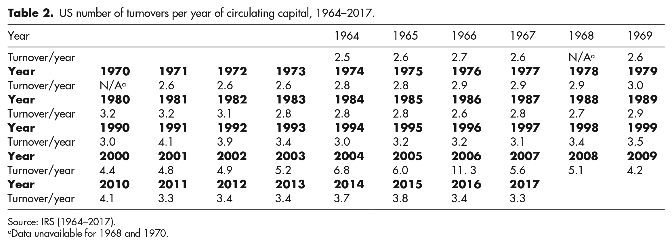
Source: IRS (1964–2017).

Data unavailable for 1968 and 1970.

The turnover of circulating capital ranges from 2.5 to 6.8 with 2006 11. 3 an anomaly reflecting the strength of the housing boom, when accounts payable was unusually larger than accounts receivable, the only year when this occurred during the entire period. The impact of just-in-time manufacturing is offset by the decline in productive activity as a proportion of total output.

US rate of profit, 1964–2017

All the components are now in place to estimate the rate of profit. Output is limited to Private Corporations, taken from the BEA (2021) Database Section 6, Income and Employment by Industry, Domestic Profits Before Tax table 6.17 and Wages and Salaries table 6.3. Turnover, Depreciable Assets Less Depreciation/Turnover or Fixed Capital Advanced (FCA), Inventories and COGS/TD are taken from the IRS (1964–2017). The proportion of COGS/TD in GO, indicates the proportion of output that produces a product and so turns over. This is assumed to be the proportion of productive and unproductive variable capital.

The total of the variables domestic profits (DP), inventories (I), fixed capital advanced (FCA), productive variable capital and unproductive variable capital (DP + I + FCA + PVC/T + UVC) is the total of value included in the rate of profit calculation. Productive variable capital (PVC) is the proportion of wages that produce an output (COGS/TD) and is divided by turnover (PVC/T) to produce the amount of productive variable capital advanced (PVCA). The proportion of productive variable capital is larger than the proportion of unproductive variable capital (UVC), but as UVC is not divided by turnover, UVC appears as larger than PVCA in the rate of profit calculation. This is the distinction between the organic composition of capital and the value composition of capital, that is, the organic composition of capital including turnover. Further investigation of this lies beyond the scope of this article.

The proportions of these are shown in Figure 1.

Figure 1.

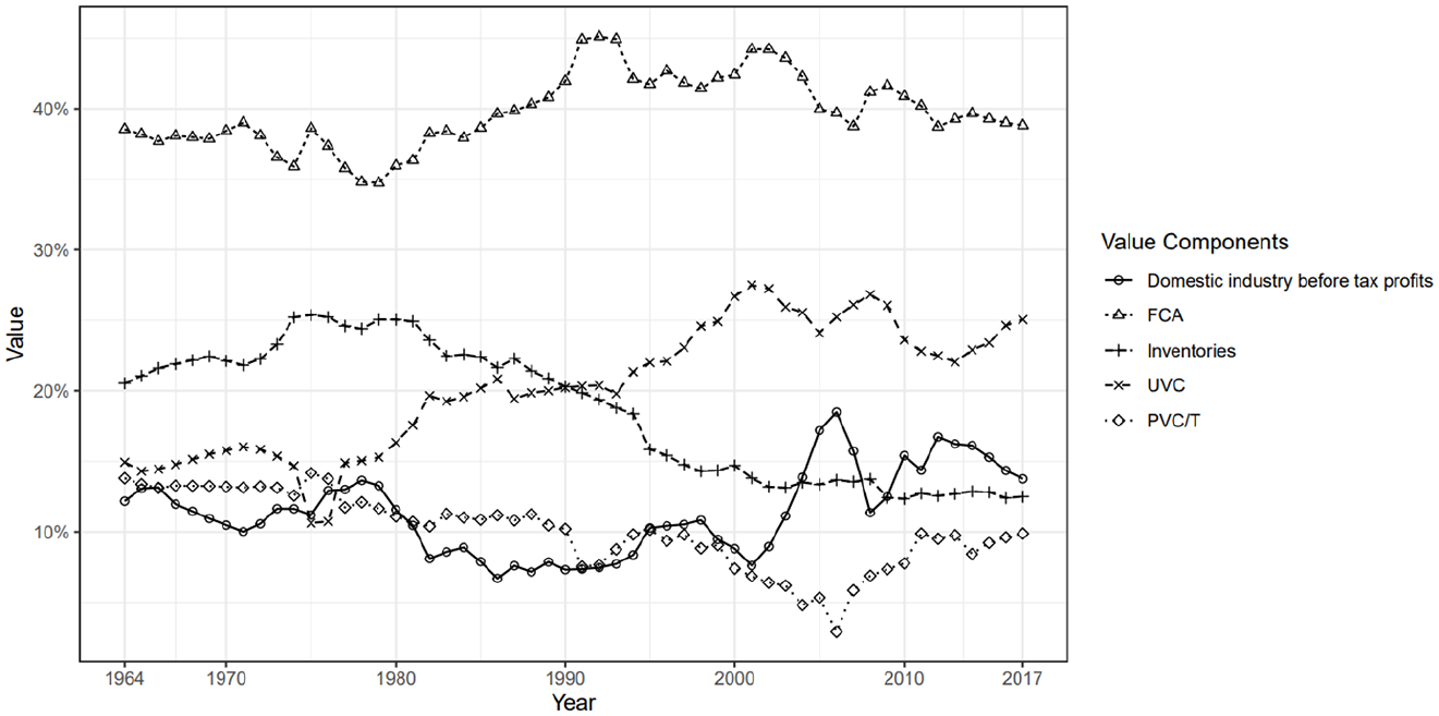
The components of surplus value and capital advanced in the rate of profit, 1964 to 2017.

The largest part consists of fixed capital advanced. Indeed, the rise in the proportion of fixed capital from the late 1970s to early 1990s coincides with the general crisis of profitability demonstrated in Figure 2. However, unlike the SNA figure which includes profits as costs, the FCA has declined through the period of globalisation from around 1990 onwards, reflecting both the deindustrialisation of the United States during the Reagan years and later offshoring with the transition of the centrally planned economies to the market. This led to generally lower domestic investment as domestic capacity declined alongside rising imports of manufactured goods. Inventories decline from the early 1980s onwards no doubt reflecting just-in-time management and lean production methods. Productive variable capital advanced falls until 2008, whereafter it recovers somewhat due to the factors described above and the rise in turnover which peaked in 2006 but then slowed towards the early 1990s levels. Domestic profits rise strongly from 2000 onwards, peaking in 2006 but then remaining elevated, reflecting very high- and rising-income inequality statistics. From these variables the formula for the rate of profit can be derived.

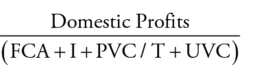
\frac{Domestic Profits}{(FCA + I + PVC / T + UVC)}

This produces the graph shown in Figure 2.

Figure 2.

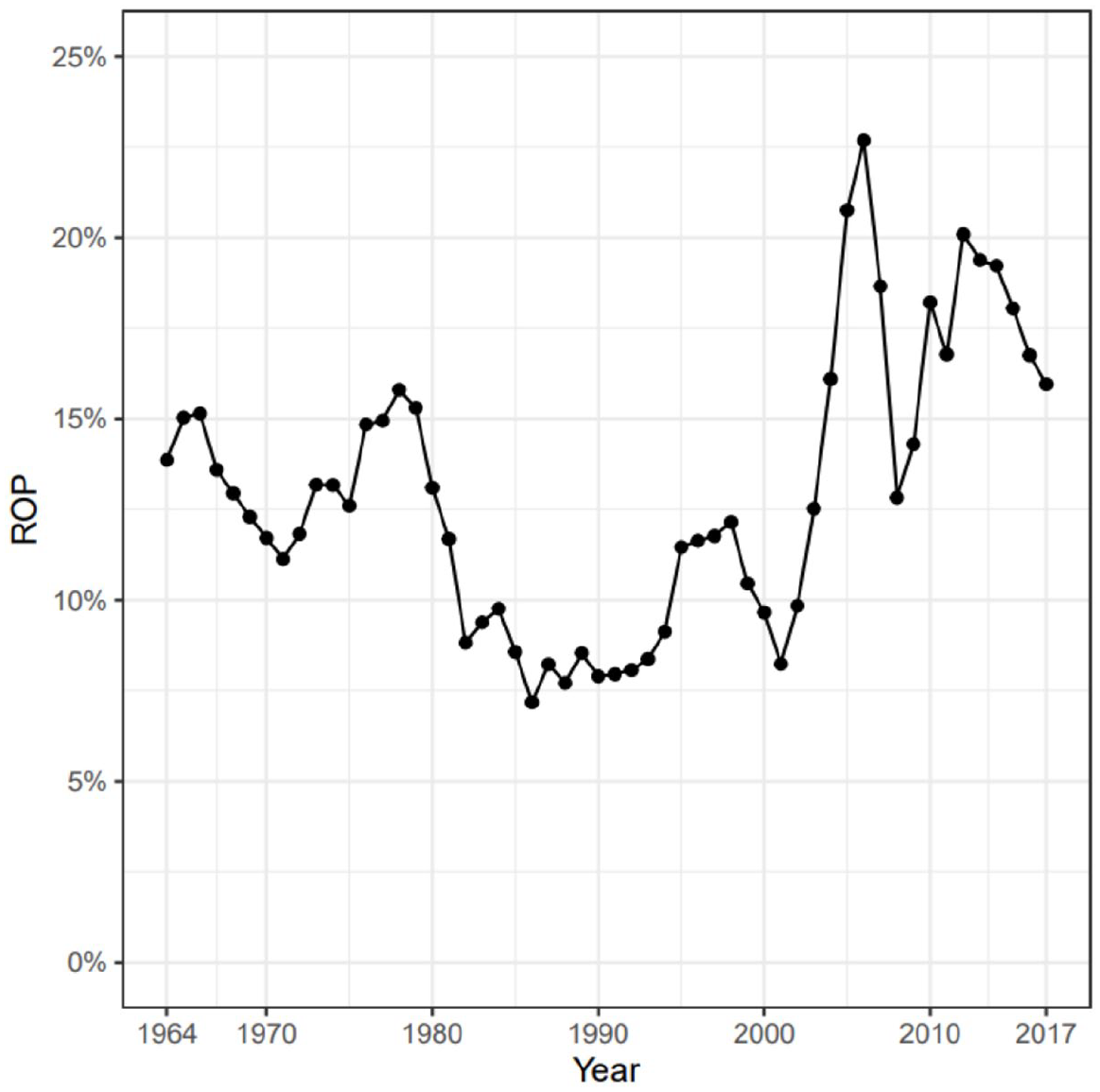
The US rate of profit, 1964–2017.

The upward trend in profit rates through the period of globalisation, but particularly after China’s accession to the World Trade Organization (WTO) in 2001 shows the limited success of the neoliberal counter revolution during the 1980s. Much more fundamental was the impact of the restoration of capitalism in the Former Soviet Union, Central and Eastern Europe after 1991 and the transition of China to a market economy by the mid-1990s (Jefferies 2015). China’s entry into the WTO in 2001 led to the strongest period of growth in profit rates in the post-war period up to the Great Recession of 2008 with the bursting of the housing bubble. Profit rates fell afterwards but remained far above their 1980s levels. The high profit rates of globalisation explain the relative ease with which US capital was able to shoulder the burden the very deep COVID-19 recession of 2020–2021. Detailed examination of the data lies beyond the scope of this article.

Conclusion

The quantity of capital advanced forms the denominator of the rate of profit calculation. The use of neoclassical valuations of the fixed capital stock grossly overestimates that value. These neoclassical estimations are not a measure of capital advanced, but of revenues generated by new investments. As Joan Robinson noted, they treat profits as a cost, so paradoxically, as profits rise profit rates fall. The IRS’ depreciable capital less depreciation provides the actual amount of capital advanced; it is around 4.5 times lower than the BEA’s historical cost fixed capital stock.

The quantity of circulating capital advanced depends on the cost of the circulating capital, raw materials and labour, and the number of circuits of capital M . . . C . . . P . . . C’ . . . M’ in a year. This circuit is conceptually linear, but its stages exist in parallel, overlapping or in a different order; customers may pay for goods before they have been produced or suppliers may deliver goods before they have been paid for (although the extent of this is limited by the physical reality of the production process). Capitalists seek to maximise profitability by using inputs before they pay for them. While the existence of unproductive sectors like finance, or departments like marketing, administration and management limits the overall turnover rate, as these sectors produce no product and so do not turnover.

Lacking any empirical evidence, or estimates that were incomplete, lacking data and conceptually inadequate, theorists have assumed that turnover was so fast as to reduce the value of circulating capital to a negligible quantity or created estimates that were unconvincing and wrong. Webber and Rigby (1986) produced broadly correct estimates for turnover in Canadian manufacturing, albeit their method was flawed. Haas (1992) applied the turnover of working capital to estimate turnover rates with the IRS data from 1964 to 1984, but this measure excluded the difference between accounts payable and accounts receivable, a key limitation on the rate of turnover. The use of neoclassical estimates of the fixed capital stock that used economists’ depreciation rates that grossly overestimated the value of the fixed capital stock meant that they lacked the motivation to discover a rigorous method for ascertaining the rate of turnover.

Bertrand and Fauqueur (1978) develop the necessary formulas for determining turnover, except for the difference between accounts receivable and accounts payable. This is included in the CCC or net operating cycle (NOC). These formulas when applied to the aggregate accounting quantities published by the IRS provide a measure of turnover. Turnover for total corporations normally fluctuates between three and six times a year, although in 2006 at the peak of the housing boom it reached nearly 12, when the typical relationship between accounts payable and accounts receivable fleetingly inverted. The rate of profit from this calculation shows that the period of globalisation, particularly during the high period of globalisation after 2001, has not been one of profitability crises but of dramatically rising profit rates, notwithstanding wild fluctuations after 2006.

Supplemental Material

sj-xlsx-1-cnc-10.1177_03098168221084110 – Supplemental material for The US rate of profit 1964–2017 and the turnover of fixed and circulating capital

Supplemental material, sj-xlsx-1-cnc-10.1177_03098168221084110 for The US rate of profit 1964–2017 and the turnover of fixed and circulating capital by William Jefferies in Capital & Class

Footnotes

Statistical Appendix 1

The formulae for turnover time developed by Hugues Bertrand and Alain Fauqueur (1978) measures the duration of the turnover of circulating capital d(t) = d₁ + d₂ + d₃

d₁ (t) procurement time

d₂ (t) production time

d₃ (t) sale time

The duration of this turnover is given by the sum of the period in which raw materials are tied up, the production time and the realisation time. To the extent that these periods coincide or overlap they reduce the sum total turnover period (Bertrand & Fauqueur 1978). The various formulae are the standard variables used within accounting.

P r o c u r e m e n t t i m e d_{1} = \frac{S_{1}}{c i}

S₁ (t) stock of raw materials at t

ci (t) intermediate consumption in value per unit of time

P r o d u c t i o n t i m e d_{2} = \frac{S_{2}}{(S_{a} + c i)}

S₂ (t) stock of intermediate products in production at t

S_a (t) wage expenditures per unit of time.

R e a l i s a t i o n t i m e d_{3} = \frac{S_{3}}{p_{3} 1}

S₃ (t) stock of finished products at t

p₃ (t) exit price for finished product from inventory before the application of the margin

m (t) margin rate: sale price = p₃ (t) × (1 + m)

(Bertrand & Fauqueur 1978: 298–300).

These formulae can be linked to the accounting categories of the Internal Revenue Service (IRS) through the cash conversion cycle (CCC) or net operating cycle (NOC). The stocks of goods, before (S₁) and after (S₃) production, are combined into average inventory (AI), with S₂ derived from the period into and out of inventory. Wage (S_a) and intermediate inputs (ci) expenditures are combined into cost of goods sold (COGS). The COGS (beginning inventory plus purchases minus end inventory) measures the cost of production each year. The procurement time, including the gap between delivery and payment, where the capitalist seeks to reduce the period that paid for raw material inputs are tied up by late payment are adjusted for through the difference between accounts receivable and accounts payable (ARP-APP). While the gross margin (m(t)) is the total revenue – COGS (TR-COGS = GM).

Average inventory (AI) is the average of the beginning and end year inventory ((Beginning Inventory + End Inventory)/2). Inventory Turnover (IT) (COGS/Average Inventory) determines the Inventory Period (IP) (365/Inventory Turnover). It is the amount of time inventory remains in storage until sold. The Accounts Receivable Period (ARP) (Average Accounts Receivable/(Revenue/365)) is the time it takes to collect cash from the sale of the inventory. The Accounts Payable Period (APP) is (Average Accounts Payable/(COGS/365)) is the time it takes to pay for inventory received. An Operating Cycle (OC) (Inventory Period + Accounts Receivable Period) equals the length of time between the purchase of inventory and the cash collected from the sale of inventory. It starts with purchase, but not payment for raw materials bought on credit. The Net Operating Cycle (NOC) (Inventory Period + Accounts Receivable Period – Accounts Payable Period) or the Cash Conversion Cycle (CCC) is the length of time between paying for inventory and receiving the cash collected from the sale of inventory M . . . M’. Total Revenue less COGS equals the Gross Margin (GM) (TR-COGS = GM).

The Cash Conversion Cycle (CCC) can also be written as DIO + DSO-DPO

Days of Inventory Outstanding (DIO) (or Days Sales of Inventory (DSI)) = Average Inventory × 365/COGS

Days Sales Outstanding (DSO)) = Average Accounts Receivable × 365/Revenue

Days Payables Outstanding (DPO) = Average Accounts Payable × 365/COGS

This produces the Annual Turnover Period (ATP) = 365/CCC.

The CCC measures the average number of days it takes for capital to turnover, from paying for productive inputs (M) . . . buying inputs (C) . . . productively consuming inputs (P) . . . selling a new commodity (C’) . . .to receiving payment for it (M’) or Marx’s circuit of production M. . .C. . .P. . .C’. . .M’.

Author’s note

Dedication: Michel Husson (1949–2021), the distinguished Marxist economist, sadly died on 18 July 2021. I corresponded with Michel for many years about various questions on Marxist political economy. He responded very positively to a late draft of this article and was particularly pleased to see the prominence it gave to the work of his friend and colleague Hugues Bertrand (also sadly deceased). Michel was going to provide more detailed feedback on the piece, but he unfortunately died before he was able do so. RIP.

ORCID iD

William Jefferies

Supplemental material

Supplemental material for this article is available online.

Author biography

William Jefferies teaches economics at SOAS. His research is interested in Marxist value theory and its application to contemporary globalisation.

References

Atradius (2018) The Americas: An Increase of Overdue B2B Receivables in 2018: Atradius Payment Practices Barometer – Results June 2018. N.V. Amsterdam: Atradius.

Basu

Vasudevan

(2013) Technology, distribution, and the rate of profit in the US economy: Understanding the current crisis. Cambridge Journal of Economics 37(1): 57–89.

Bertrand

Fauqueur

(1978) Rotation du capital circulant et rentabilité. Revue Économique, Programme National Persée 29(2): 291–331.

Bureau Economic Analysis (BEA) (2003) Fixed Assets and Consumer Durable Goods in the United States 1925-97. New York: BEA.

Bureau Economic Analysis (BEA) (2021) GDP by Industry. New York: BEA. Available at: https://apps.bea.gov/iTable/index_industry_gdpIndy.cfm

Cockshott

Cottrell

(2003) Notes and comments: A note on the organic composition of capital and profit rates. Cambridge Journal of Economics 27(5): 749–754.

DOT (2000) Report to the Congress on Depreciation Recovery Periods and Methods. Department of Treasury, July 28 2000, Washington.

Dumenil

Levy

(2002) The profit rate: Where and how much did it fall? Did it recover? (USA 1948-2000). Review of Radical Political Economics 34(4): 437–461.

Fabricant

(1938) Capital Consumption and Adjustment. Cambridge, MA: National Bureau of Economic Research (NBER).

10.

Fichtenbaum

(1988) ‘Business cycles’, turnover and the rate of profit: An empirical test of Marxian crisis theory. Eastern Economic Journal 14(3): 221–228.

11.

Gill

Bigger

Mathur

(2010) The relationship between working capital management and profitability: Evidence from the United States. Business and Economics Journal 10: 1–9.

12.

Haas

(1992) Technical and organizational progress and the turnover of capital. Review of Radical Political Economics 24(1): 114–135.

13.

Hulten

Wykoff

(1981) The measurement of economic depreciation. In: Hulten

(ed.) Depreciation, Inflation, and the Taxation of Income from Capital. Washington, DC: The Urban Institute, pp. 81–125.

14.

Internal Revenue Service (IRS) (1964–2017) Statistics of Income Corporation Source Book Active Income Tax Returns; Balance Sheet, Income Statement, Tax and Selected Items by Major and Minor Industries, Size of Total Assets. New York: Department of the Treasury, IRS. Available at: https://www.irs.gov/statistics/soi-tax-stats-all-years-irs-data-books; https://www.irs.gov/statistics/soi-tax-stats-archive-1863-to-1999-annual-reports-and-irs-data-books

15.

Internal Revenue Service (IRS) (1987) Rev. Proc. 87-56, 1987-2 C.B. 674. New York: Department of the Treasury, IRS.

16.

Internal Revenue Service (IRS) (2005) Table 4. Comparison of Personal Income in the National Income and Product Accounts (NIPA) with Adjusted Gross Income (AGI), for Specified Tax Years, 1990-2005. New York: Department of the Treasury, IRS.

17.

Internal Revenue Service (IRS) (2018) How to Depreciate Property Publication (IRS, 946 (2018), 15 February 2019). New York: Department of the Treasury, IRS

18.

Jefferies

(2015) On the alleged stagnation of capitalism. Review of Radical Political Economics 47(4): 588–607.

19.

Jefferies

(2021) Capital and class rate of profit calculation 1964 to 2017 dataset. Available at: https://www.researchgate.net/publication/354477964_Capital_and_Class_Rate_of_Profit_Calculation_1964_to_2017_Dataset

20.

Jones

(2017) Turnover time and the organic composition of capital. Cambridge Journal of Economics 41(1): 81–103.

21.

Kuczynski

(1992) Great depressions as transitional phases within the capitalist mode of production. In: Kleinknecht

Mandel

Wallerstein

(eds) New Findings in Long-Wave Research. Basingstoke: St. Martin’s Press, pp. 257–275.

22.

Lapavitsas

(2000) On Marx’s analysis of money hoarding in the turnover of capital. Review of Political Economy 12(2): 219–235.

23.

Maito

(2018) The tendency of the rate of profit to fall since the nineteenth century and the world rate of profit. In: Roberts

Carchedi

(eds) World in Crisis: A Global Analysis of Marx’s Law of Profitability. Chicago, IL: Haymarket, pp. 129–156.

24.

Marx

(1966 [1894]) Capital: A Critique of Political Economy, vol. 3. London: Lawrence & Wishart.

25.

Marx

(1973) The Grundrisse. London: Penguin Books.

26.

Marx

(1978 [1885]) Capital: A Critique of Political Economy, vol. 2. London: Penguin Books.

27.

Mohr

Gilbert

(1996) Capital Stock Estimates for Manufacturing Industries: Methods and Data Industrial Output Section – Stop 82 Division of Research and Statistics Board of Governors of the Federal Reserve System 20551 (March). Washington, DC: United States Federal Reserve.

28.

Moseley

(1985) The rate of surplus value in the postwar US economy: A critique of Weisskopf’s estimates. Cambridge Journal of Economics 9: 57–79.

29.

Moseley

(1986) Estimates of the rate of surplus-value in the postwar United States economy. Review of Radical Political Economics 18(1–2): 168–189.

30.

Ochoa

(1984) Labour-values and prices of production: An interindustry study of the US economy, 1947-1972. New School for Social Research PhD Dissertation (ProQuest Dissertations & Theses Global: The Humanities and Social Sciences Collection). Available at: https://www.econbiz.de/Record/labor-values-and-prices-of-production-an-interindustry-study-of-the-us-economy-1947-1972-ochoa-edward-martin/10000687128

31.

Ochoa

(1989) Values, prices and wage profit curves in the US economy. Cambridge Journal of Economics 13: 413–429.

32.

Office for National Statistics (ONS) (2017) Payment Practices Report. London: ONS. Available at: https://www.gov.uk/check-when-businesses-pay-invoices (accessed 20 January 2020).

33.

Organisation for Economic Co-operation and Development (OECD) (2009) Measuring Capital OECD Manual. 2nd ed. Paris: OECD.

34.

Paitaridis

Tsoulfidis

(2018) The growth of unproductive activities, the rate of profit, and the phase-change of the U.S. economy. Review of Radical Political Economics 44(2): 213–233.

35.

Passarella

Baron

(2015) Capital’s Humpback Bridge: ‘Financialization’ and the rate of turnover in Marx’s economic theory. Cambridge Journal of Economics 39(5): 1415–1144.

36.

Reati

(1992) Comment: Long waves in profit rates in four countries. In: Kleinknecht

Mandel

Wallerstein

(eds) New Findings in Long-Wave Research. Basingstoke: St. Martin’s Press, pp. 168–174.

37.

Richards

Laughlin

(1980) A cash conversion cycle approach to liquidity analysis. Financial Management 9(1): 32–38.

38.

Roberts

Carchedi

(2018) The long roots of the present crisis: Keynesians, Austerians and Marx’s Law. In: Roberts

Carchedi

(eds) World in Crisis: A Global Analysis of Marx’s Law of Profitability. Chicago, IL: Haymarket, pp. 13–35.

39.

Robinson

(1953) The production function and the theory of capital. The Review of Economic Studies 21(2): 81–106.

40.

Saros

(2008) The turnover continuum: A Marxist analysis of capital fluctuations. Review of Radical Political Economics 14(2): 189–211.

41.

Sato

(2018) Japan’s ‘lost’ two decades: A Marxist analysis of prolonged capitalist stagnation. In: Roberts

Carchedi

(eds) World in Crisis: A Global Analysis of Marx’s Law of Profitability. Chicago, IL: Haymarket, pp. 157–183.

42.

Shaikh

(2016) Capitalism; Competition, Conflict, Crises. Oxford: Oxford University Press.

43.

Spulber

(1964) Foundations of Soviet Strategy for Economic Growth. Bloomington, IN: Indiana University Press.

44.

Strassner

Medeiros

Smith

(2005) Annual Industry Accounts Introducing KLEMS Input Estimates for 1997–2003. New York: BEA. Available at: https://apps.bea.gov/scb/pdf/2005/09September/0905_Industry.pdf

45.

Tsoulfidis

Tsaliki

(2019) Classical Political Economics and Modern Capitalism; Theories of Value, Competition, Trade and Long Cycles. London: Springer.

46.

Webber

Rigby

(1986) The rate of profit in Canadian manufacturing, 1950–1981. Review of Radical Political Economics 18(33): 33–55.

47.

Weisskopf

(1979) Marxian crisis theory and the rate of profit in the postwar U.S. economy. Cambridge Journal of Economics 3(4): 341–378.

Supplementary Material

Please find the following supplemental material available below.

For Open Access articles published under a Creative Commons License, all supplemental material carries the same license as the article it is associated with.

For non-Open Access articles published, all supplemental material carries a non-exclusive license, and permission requests for re-use of supplemental material or any part of supplemental material shall be sent directly to the copyright owner as specified in the copyright notice associated with the article.

0.00 MB

0.10 MB