
Abstract
Fatigue loads are becoming a limiting factor of modern wind energy turbines with increasing rotor diameters and hub heights. This applies especially to the blade root, where bending moments caused by cyclic loads, such as the vertical wind gradient, gusts, turbulence and other periodic inputs, reach their maximum value. Reducing these bending moments is therefore helpful to allow further growth of blade length and power rating of future turbines. One way to reduce these loads is provided by actively controlling the trailing edge at the outer part of the blade. This influences the lift and by this the root bending moment. In this paper, the experimental test results of a morphing, flexible trailing edge flap will be presented. The crucial advantage of the morphing mechanism consists in the possibility to keep the trailing edge completely sealed to the environment. This prevents the ingression of water, dust or insects which could cause excessive wear at the mechanism. This flexible trailing edge has been experimentally investigated within a wind tunnel and on a rotating test rig in real wind conditions. This paper will provide brief information about the design of the two-meter span test demonstrator, the instrumentation, and test setup. The main goal of both tests was the measurement of the flap polars to quantify the lift change caused by a deflection of the flexible trailing edge. In addition, a sensor controlled movement of the trailing edge was implemented in the rotation test with the aim to reduce the bending moment. Three different signals—the rotor azimuth, the angle of attack and the bending moment itself—have been used as a reference. The reduction of the bending moment could be demonstrated successfully for all three reference signals.
Introduction
Decreasing resources of fossil energy and rising carbon dioxide levels in the atmosphere lead to an increasing need for renewable energy supply. Wind energy is one key component since it can be harvested on any location with sufficient wind. Since the yield of wind energy increases with the rotor area and the height of the turbine, the sizes of these turbines have been increased in the last decades. This allows to use the potential locations of wind turbines much more efficiently in comparison to smaller installations hence resulting in reduced energy cost and land consumption.
The growing size of modern turbines however raises a challenge: Fatigue loads. Wind gradients, gusts and turbulence, the transition of the blade in front of the tower, and even the changing orientation of the blade to the gravitation produce angle of attack and inflow speed variations on the rotor blade. These variations eventually result in cyclic bending moments in the blade root. If the turbine gets bigger, the load due to mass and gravitation becomes more important since the mass grows faster than rigidity. Reducing these bending moments could also reduce the fatigue stress in the blade. An effective way of achieving this is to change the angle of attack on the blade according to the inflow conditions. This can either be done for the entire blade or only for blade section.
In the case of Individual Pitch Control (IPC), the pitching system of each blade is used to change the angle of incidence individually Larsen et al. (2005) and by this the angle of attack on the entire blade. This is quite easy to implement, since all modern wind turbines have a pitch system to tilt the blades according to the inflow conditions, but it is easy to understand that the mass of the whole blade has to be moved. Therefore, the maximum frequency, at which an IPC can be implemented, is limited. On the other hand, Individual Flap Control (IFC) changes the angle of attack only for a blade section at the outer part of the blade. Since its mass is much smaller in relation to the entire blade, it can be moved significantly faster. Using this approach, different research groups have undertaken investigations in the field of trailing edge devices ranging from simulations, wind tunnel tests or even tests on turbines. Since an in depth literature is not focus of this paper, more information about previous projects and existing work can be found in Barlas and Van Kuik (2010) and Pohl and Riemenschneider (2023).
At DLR, a flexible trailing edge has been developed for IFC on wind turbine blades. The flexible, morphing approach implementing elastomer covers has been used to be able to fully seal the inner components of the flap against environmental influences, such as water, dust or insects. This paper will provide some brief information about the design of the trailing edge. Details on the design and laboratory testing of this flap can be found in Pohl and Riemenschneider (2023). The main focus of the paper lies on the experimental investigation of the trailing edge. It has been tested in a wind tunnel at the University of Oldenburg as well as on an outside rotating test rig in real wind conditions at the Danish Technical University in Risø.
In the wind tunnel and rotating tests, it could be demonstrated, that moving the trailing edge changes the lift coefficient of the airfoil as expected. The lift polars of the trailing edge flap have been measured in both test setups. Furthermore in the rotating test, a reduction in the bending moment of the boom, where the test demonstrator was mounted, was demonstrated even with comparably simple proportional feedforward and feedback control methods.
Design of flexible trailing edge and test demonstrator
The fundamental concept of the flexible trailing edge flap is based on a design using three fiber composite layers with quadrilateral inner cells. Two of the three composite layers form the upper and lower aerodynamic surface of the airfoil while the third layer is placed in the skeleton line. Due to the quadrilateral shape of the inner cells, they do not block a shear deformation. That is why the whole trailing edge can be bent upward or downward. Figure 1 shows a cross-section of the final design. Cross-section of the flexible trailing edge.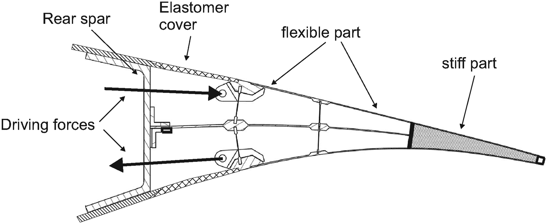
The concept uses opposite driving forces shown on the brackets in Figure 1. From there the forces are transferred by the outer fiber composite layer. The inner layer has been tailored in a way to allow bending while simultaneously transferring the aerodynamic shear forces to the rear spar, where the trailing edge is mounted. To allow a deformation, the brackets, where the driving forces are introduced, need to move several millimeters in chordwise direction. Since a pure fiber composite skin is too stiff to allow the required strains, elastomer covers are used to close these gaps. By this, there is no need for slots to allow a movement of the trailing edge, which allows to fully seal the mechanism. For the demonstrator, the DU91-W2-250 airfoil has been used which can be seen as representative for the outer region of wind turbine blades. In Figure 2, the CAD model (a) and a photo of the fabricated trailing edge prototype (b) are shown. Flexible trailing edge for rotation test at DTU.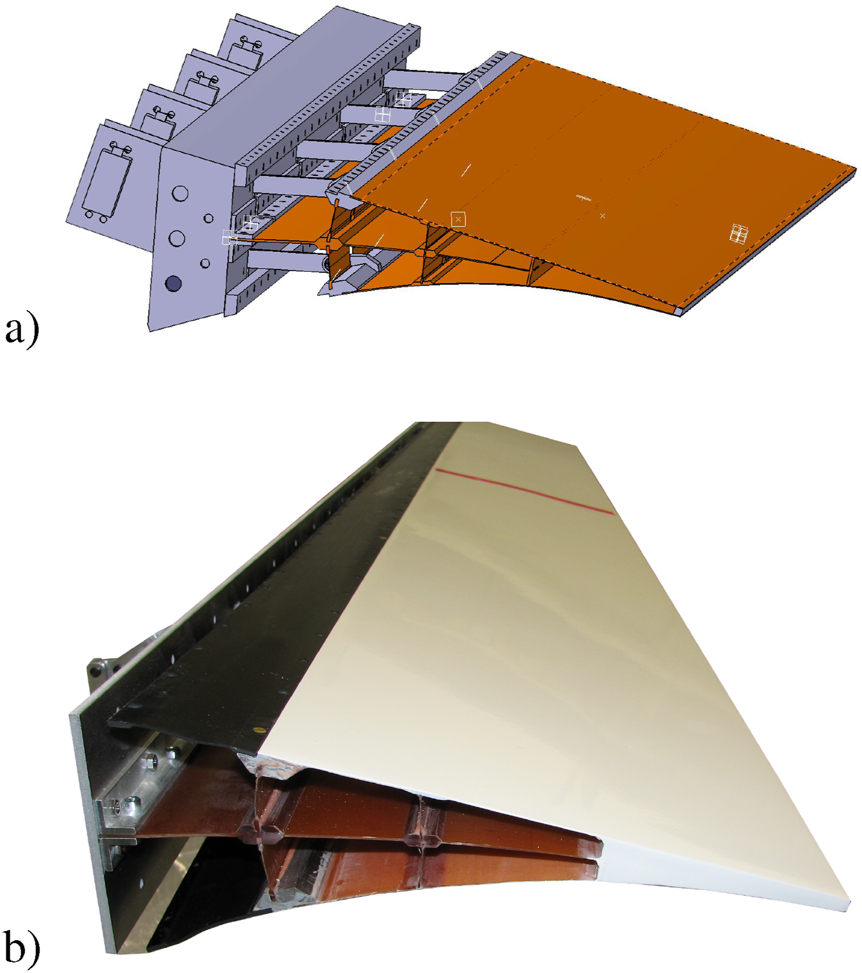
With this prototype, laboratory tests have been made to test the deflection behavior. More information about the design process and the results of the lab tests are provided in Pohl and Riemenschneider (2023).
In the beginning, it was intended to use the elastomer gap covers (the black parts in Figure 2) between the rear spar and the flexible trailing edge for all tests. Unfortunately the elastomer cracked shortly before the rotation test. Due to a lack of time to redesign and refabricate the elastomer covers, a sliding cover was designed and built to perform the rotating test, which is shown in Figure 3. It is made from two parts as shown in the figure. The left part used on the upstream side is made from two 0.5 mm glass fiber layers on the upper and lower side. Between them is a 1 mm gap, where the part shown on the right side of the figure slides in. This part has a thickness of 1 mm which results in a tight fit. By this a small 0.5 mm step is created at the end of the upper layer of the upstream part of the sliding cover. Sliding gap cover of trailing edge partially separated.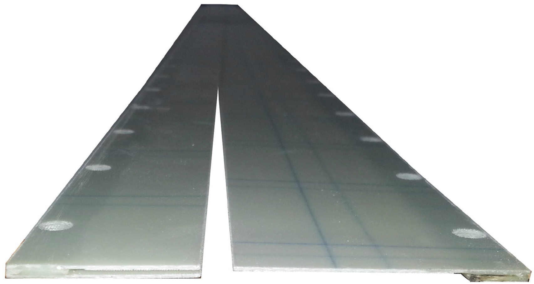
Since the wind tunnel test was conducted later, a new elastomer cover was designed and built and successfully tested.
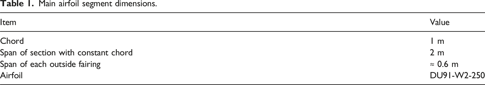
In parallel to the design of the trailing edge, the rigid part of the demonstrator was designed. Figure 4 shows the CAD model of this part with the trailing edge attached in the rear. Since the rotation test is conducted at the test rig of Danish Technical University (DTU), the design and fabrication of the rigid part of the airfoil was done there. The rigid part of the airfoil was fabricated to a tolerance of less than 0.2 mm between the gaps of the leading edge and the upper and lower covers. Additionally, the gaps were covered with thin tape during the tests. CAD model of airfoil section.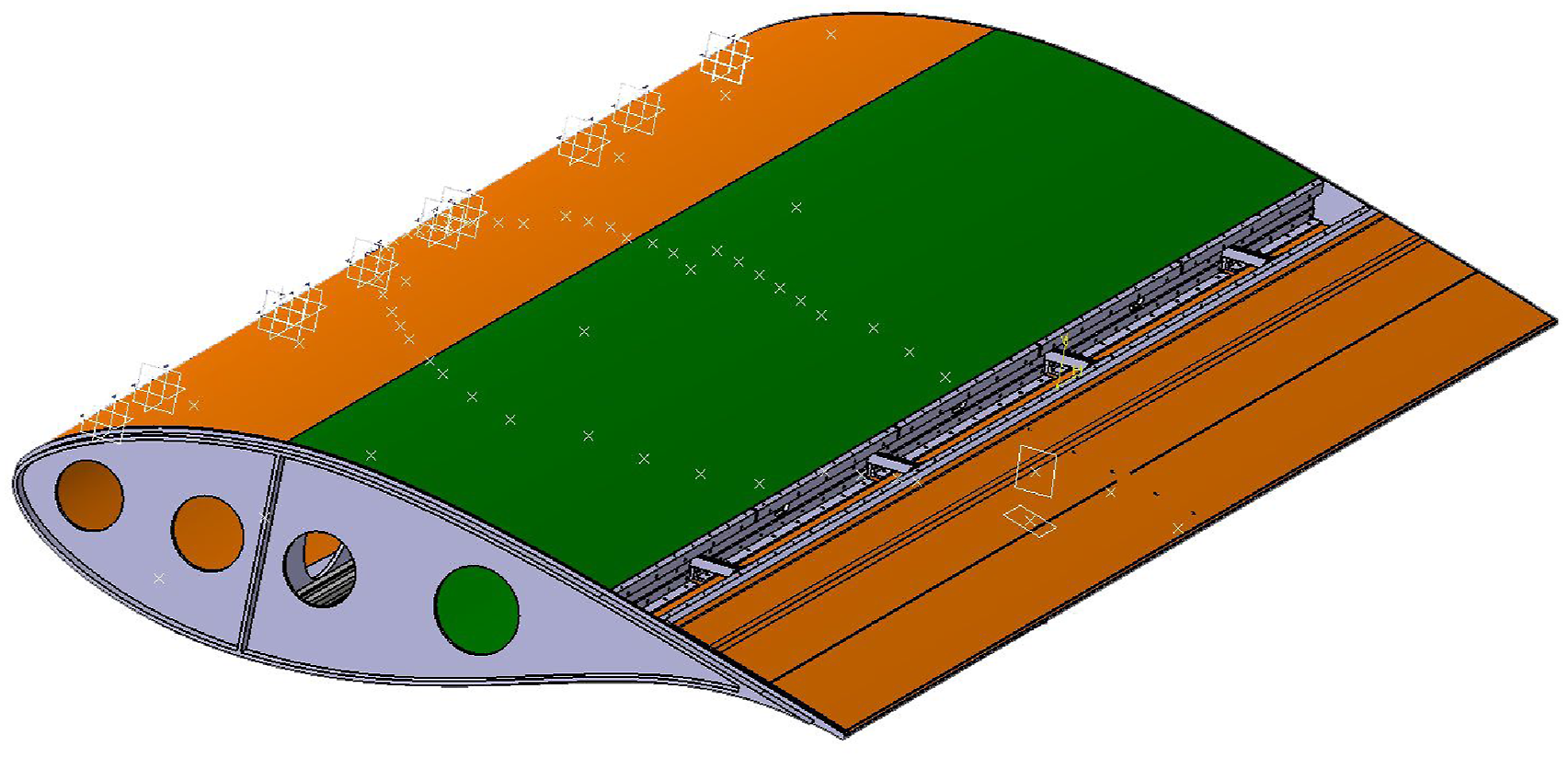
Main airfoil segment dimensions.
Experimental investigation
Overview
As already mentioned in the introduction, a wind tunnel test and a rotating test in a specialized test rig are performed to investigate the flexible trailing edge in a controlled flow and in real wind conditions. Hereby it would have been logical to finish the wind tunnel test before performing the more challenging and realistic rotating test. This was unfortunately not possible since the wind tunnel construction was not finished until short before the end of the project. Therefore, the rotating test had to be carried out before the wind tunnel test.
Instrumentation of trailing edge and airfoil segment
A variety of different structural and aerodynamic sensors have been implemented within the demonstrator to measure the effect of the trailing edge on the aerodynamics and the movement of the airfoil. The following list contains all implemented sensors: • 57 strain gauges at the trailing edge structure • 3 three axis accelerometers to obtain the movement of the whole airfoil segment • 2 one axis accelerometers in the trailing edge • 64 pressure taps, where 52 are located chordwise in the middle of the airfoil and 12 spanwise • servo angle measurement at all driving servos of the trailing edge • two five-hole probes at the leading edge of the test section to measure inflow speed and angle of attack used in the rotation test
For data acquisition and trailing edge control, a National Instruments cDAQ 9135 system with different modules for the individual sensors was mounted inside the demonstrator. To cover a wide frequency range, the strain gauges are measured with a sampling frequency of f strain = 1 kHz, whereas the accelerometers were sampled with f strain = 2048 Hz. The positions of the servo motors were obtained with a frequency of f servo = 30 Hz. All other data have been acquired with a frequency of f = 100 Hz.
To power the servo motors and the data acquisition system, two voltages of 8.4 V and 21 V are needed. Since the servo motors are drawing up to 15 A peak current and are able to work as generators, a lithium polymer battery was installed as a buffer. This high driving current allows to use the full speed of the servos resulting in a maximum flap speed of 47 o /s. Also the power supply for the data acquisition system was buffered with a battery to prevent power losses.
Eight model aircraft servo motors (Hitec HSB3980) are used in parallel to drive the trailing edge. To obtain the servo angle, the internal position feedback potentiometer is used resulting in values between 0 and 1500 for the full 180 o stroke. Therefore, an angular resolution of 0.12 o is achieved. This servo angle position is also used to obtain the flap angles according to Figure 17 in Pohl and Riemenschneider (2023) where the trailing edge was measured in the lab.
Figure 5 shows a photo of the opened demonstrator with the data acquisition system and the power supply installed. The free space on the left side is used by the pressure transducers of the surface pressure taps, which are installed individually for the wind tunnel test and the rotation test. Measurement instrumentation of the segment demonstrator.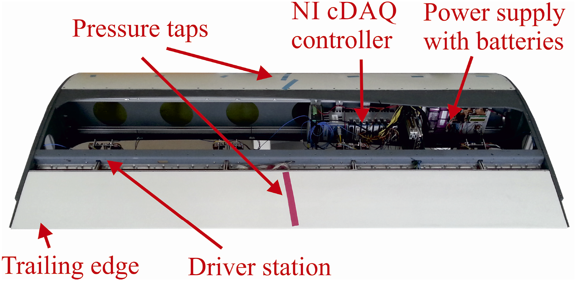
Rotation test
Setup at test rig
The field research test rig is situated at the Danish Technical University (DTU) at its wind energy research site Risø. It consists of a Tellus T-1995 wind turbine, where the rotor blades including the blade hub have been removed from the rotor shaft. Instead, a boom was designed, where a test airfoil section can be mounted and rotated for measuring in real wind conditions. To compensate the mass of boom and test section, a counterweight was added to the other side.
This paper will not further consider the design of the test rig itself since the report of the INDUFLAP project covers all relevant information, see Barlas and Aagaard Madsen (2014). Figure 6 shows the whole test rig in the upper image (a) with the segment demonstrator from this paper attached to the boom. In the lower image (b), a detail view of the segment demonstrator is shown. There, two five-hole probes can be seen on the leading edge in the upper left part of the image, which have been added to measure the inflow angle to the airfoil section and the stagnation pressure. They are each mounted at 0.5 m distance from the spanwise center where the pressure taps are located and reach 0.45 m upstream. The angle of attack (AoA or α) was calculated based on the five-hole probe data by subtracting the offset angle between the five-hole probes and the blade chord from the five-hole probe data and averaging between the two probes. The trailing edge is visible on the other side of the airfoil behind the second green line. Full view of test rig with attached segment demonstrator (a) and detail view of segment demonstrator (b).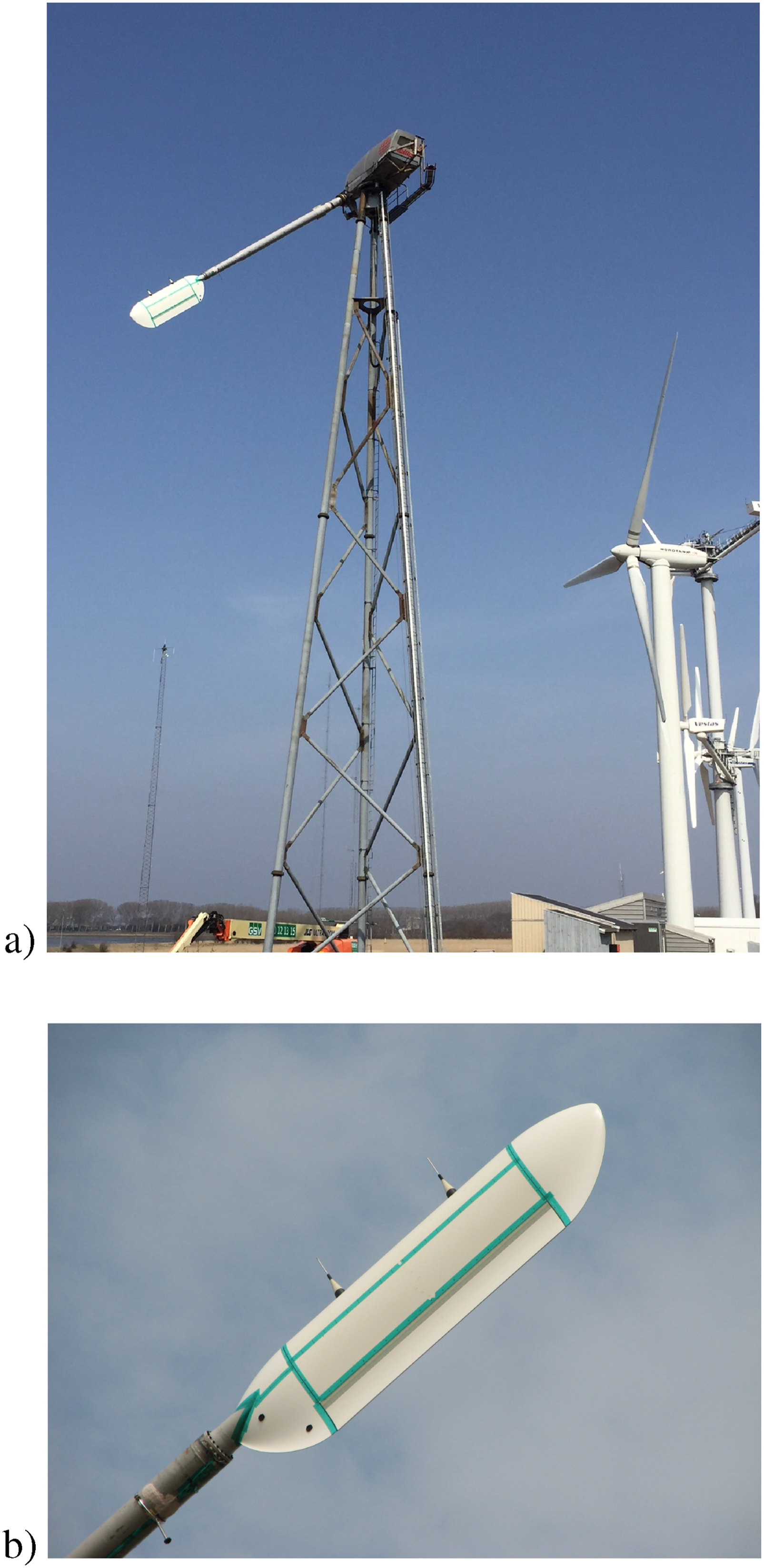
To measure the inflow characteristics and the movements, the test rig is equipped with a variety of sensors. Additionally, a met mast is placed west of the rotating test rig in the main wind direction to measure the inflow. The following sensors are installed on the test rig and the met mast: • Bending and torsion moment sensors in boom • Rotor Azimuth and yaw angle sensor of rotor hub • Met mast (sensor tower upstream of the test rig) with wind speed, wind direction and temperature sensors west of test rig
To obtain images of the moving trailing edge during rotation, mounting points for small action cameras have been added to the airfoil. They can be seen in Figure 6 in the right image as the small black spots at the inner fairing of the segment demonstrator, where the boom is attached. Based on these films, a visual inspection of the flexible trailing edge flap movement in different conditions is possible. Figure 7 shows two captured images of the flap being fully negative (upper part) and positive displaced while in full rotation. Flap deflection: full negative (upper) and full positive (lower).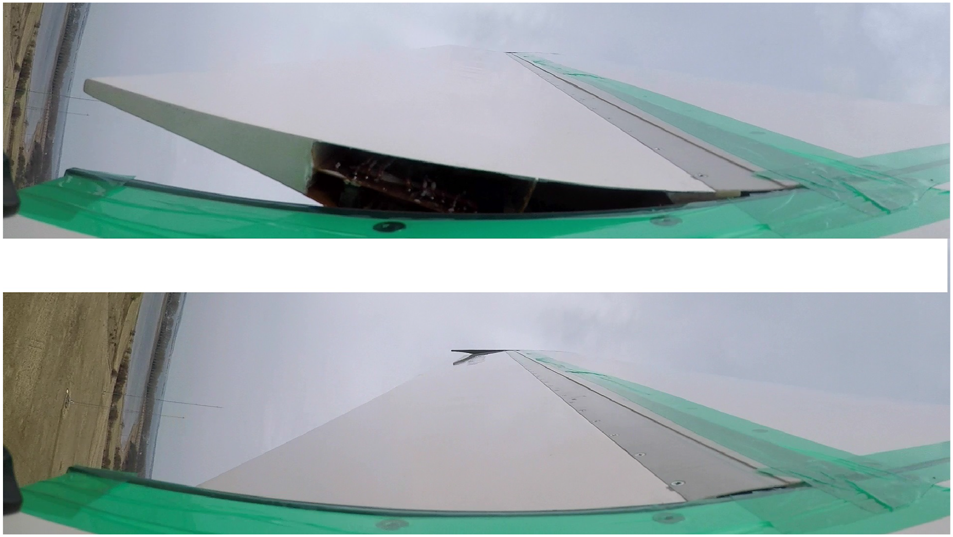
The measurements itself took place from April 09 to April 20 2018. These 2 weeks were dominated by a meteorological high pressure system, where the measurement site was at the southern part of the system in the first week with high wind speeds from eastern directions. In the second week, the wind calmed down as the system left to the east changing the wind direction more to the west. Due to the high wind speeds in the first week, measurements were suspended since the possible pitch was not big enough to keep the angle of attack of the demonstrator in a usable range. Therefore, the presented data are solely measured in the second week. More information on the meteorological conditions can be found in the Appendix. The diagrams of ambient pressure and the distribution of wind speed, wind direction can be seen in Figures 30–32 in the Appendix.
Although the test rig is capable of a maximum rotation speed of 50 rpm, this was limited to 20 rpm for the measurement campaign to avoid running through critical speeds and resonances. This results in an inflow speed of around 20 m/s due to rotation. Angles of attack of the airfoil between −10 o and 20 o have been measured.
Flap polars
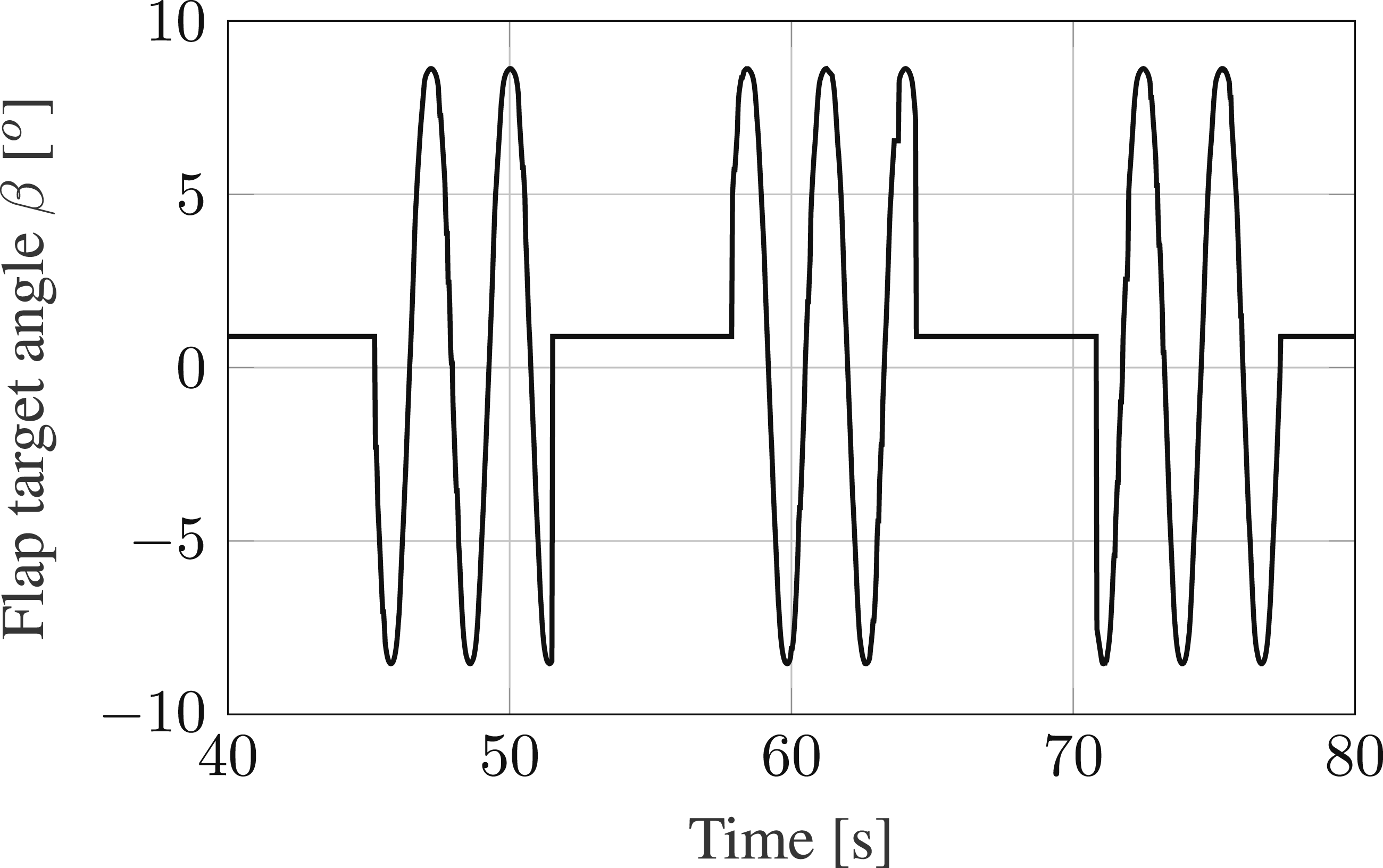
To calculate the lift of the airfoil and subsequently the flap polars, the chordwise pressure taps in the spanwise mid of the airfoil demonstrator are used. In order to allow comparable wind situations, the flap angle β is deflected in a stepwise manner, where each step starts from neutral position without deflection, then to the desired positive flap angle, back to neutral, followed by the desired negative angle and back to neutral. This stepwise signal of the trailing edge flap angle can be seen in Figure 8 for a measurement setting with full deflection of β ≈ ± 8.5
o
. Each step is kept constant for 15 s. Further measurements have been done with −5.5
o
to 6.8
o
and −2.2
o
to 4.3
o
. The latter values correspond to approximately two thirds and one third of the maximum deflection angle of the trailing edge. This provides information about the whole deflection range of the trailing edge flap. The slight offset of the neutral position arises from the fact that the rotation angles of the servo motors were chosen to be the positive and negative full stroke, two thirds of the full stroke, one third of the full stroke, and the neutral middle position of the servo motor. Since the flap does not fully behave linearly due to the eccentric driving kinematics, the mentioned flap deflection angles follow out of these servo positions. The exact characteristic curve of the driving mechanism can be found in Pohl and Riemenschneider (2023). Example trailing edge flap target angle for flap polar measurements with full flap stroke.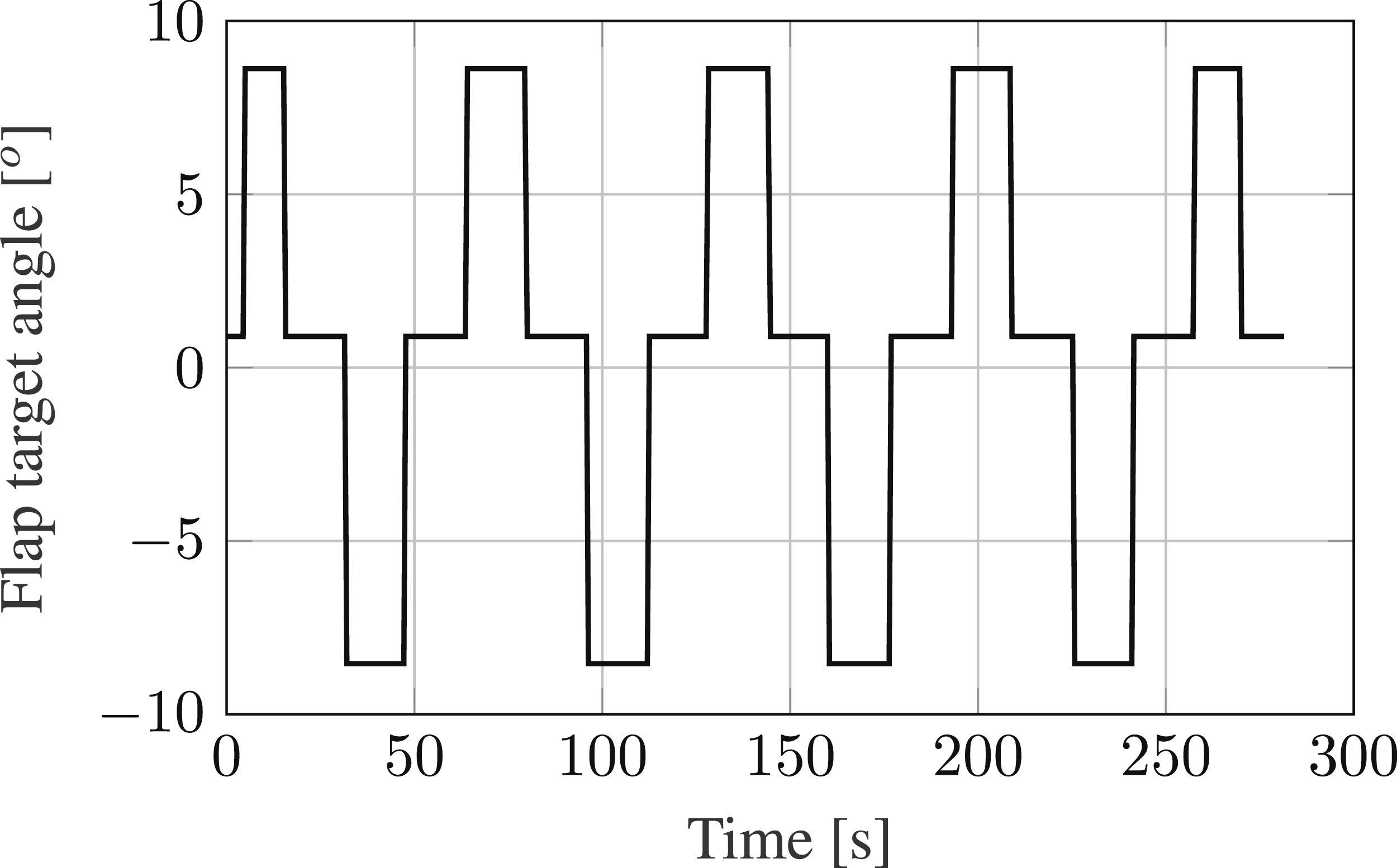
When looking at the time signals of some exemplary pressure taps shown in Figure 9, two fundamental patterns can be seen in the pressure curves. First the deflection of the trailing edge flap is visible since the pressure values follow a 15 s step pattern. Second in each 15 s time period five additional fluctuations of the pressure signal are visible. These are caused by the rotation of the test rig in the vertical wind gradient. Since one revolution takes three seconds this results in five peaks of the pressure signal. These fluctuations are resulting from different inflow velocities due to the vertical wind gradient, which lead to variations in dynamic pressure and angle of attack. Hence, changes in the chordwise pressure distribution occur. Surface pressure variations.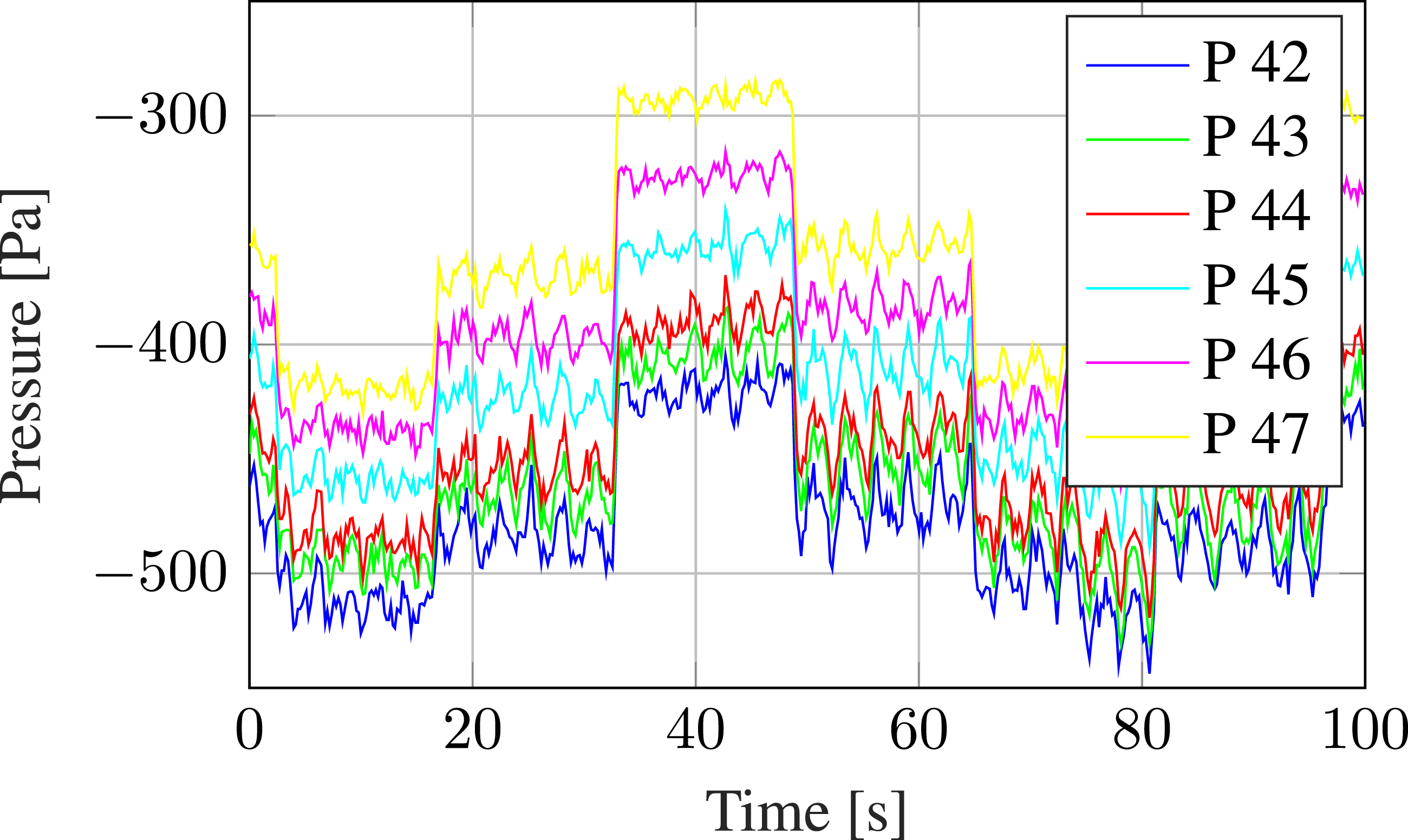
To calculate the lift coefficient based on the measured pressure data, the pressures are integrated over the chord of the airfoil. A sketch of the method can be seen in Figure 10. The normal vector Sketch of c
L
calculation.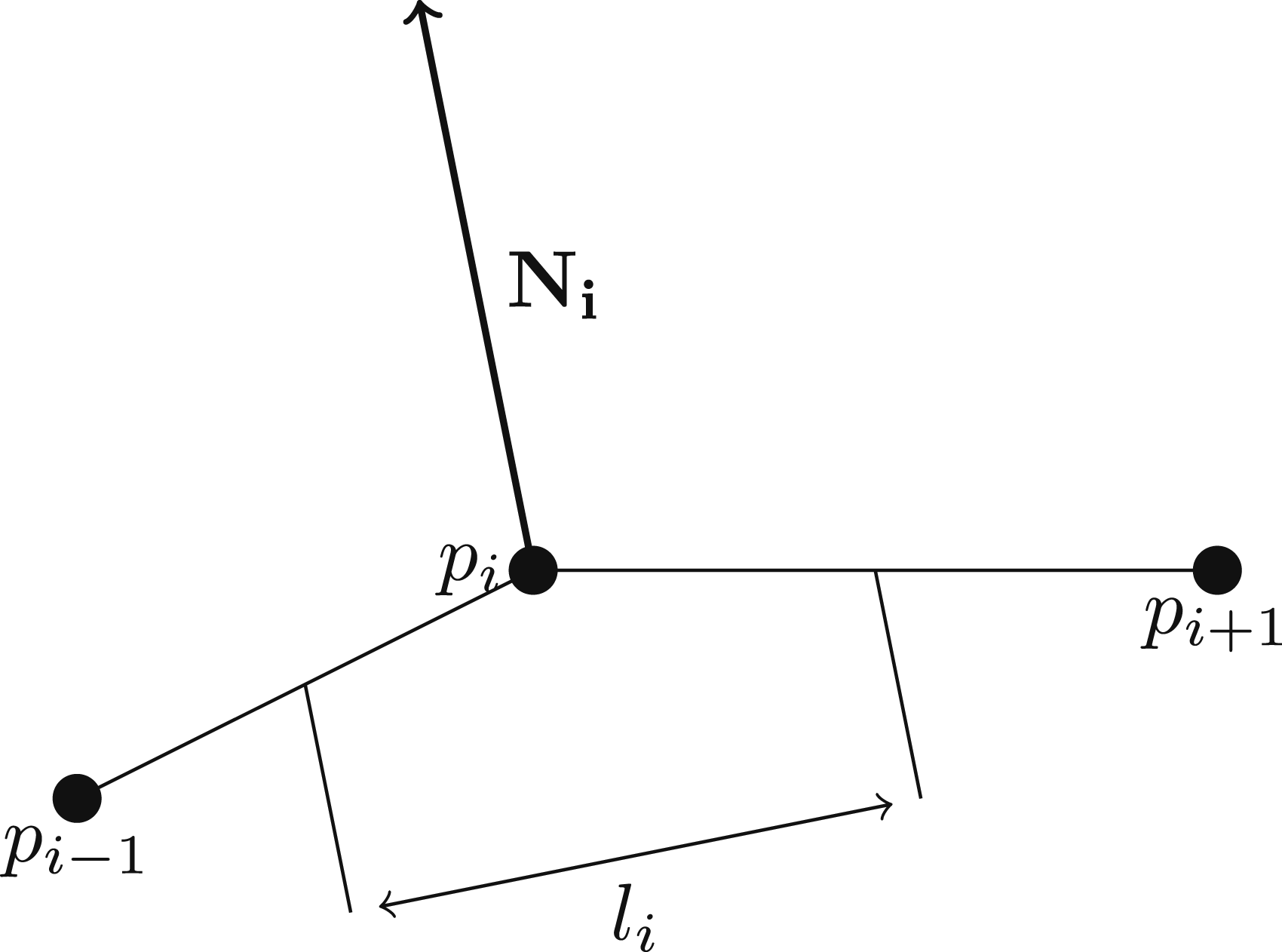
Since the lift is the component perpendicular to the chord, only the second part of the normal vector is of interest. Equation (1) shows the calculation of the lift coefficient with c as the chord length of the airfoil. Not that the results shown in the following diagrams base on this equation. There have no further manipulations of the data been done in order to, for example, compensate the finite span of the airfoil section.
Combining several measurements with different pitch angles and inflow conditions, a wide angle of attack area can be covered. This process is done for each flap deflection angle. One example of a combination of 13 measurements with a flap angle of β = 6.8
o
is shown in Figure 11, where measurements have been performed on different days. There the individual measurements are shown in different colors. As expected, c
L
rises with increasing α. Additionally, due to the stochastic nature of the inflow conditions in natural wind, the c
L
values are noisy. Raw measurement data (500 samples each measurement) for all measurements with 6.8
o
trailing edge angle.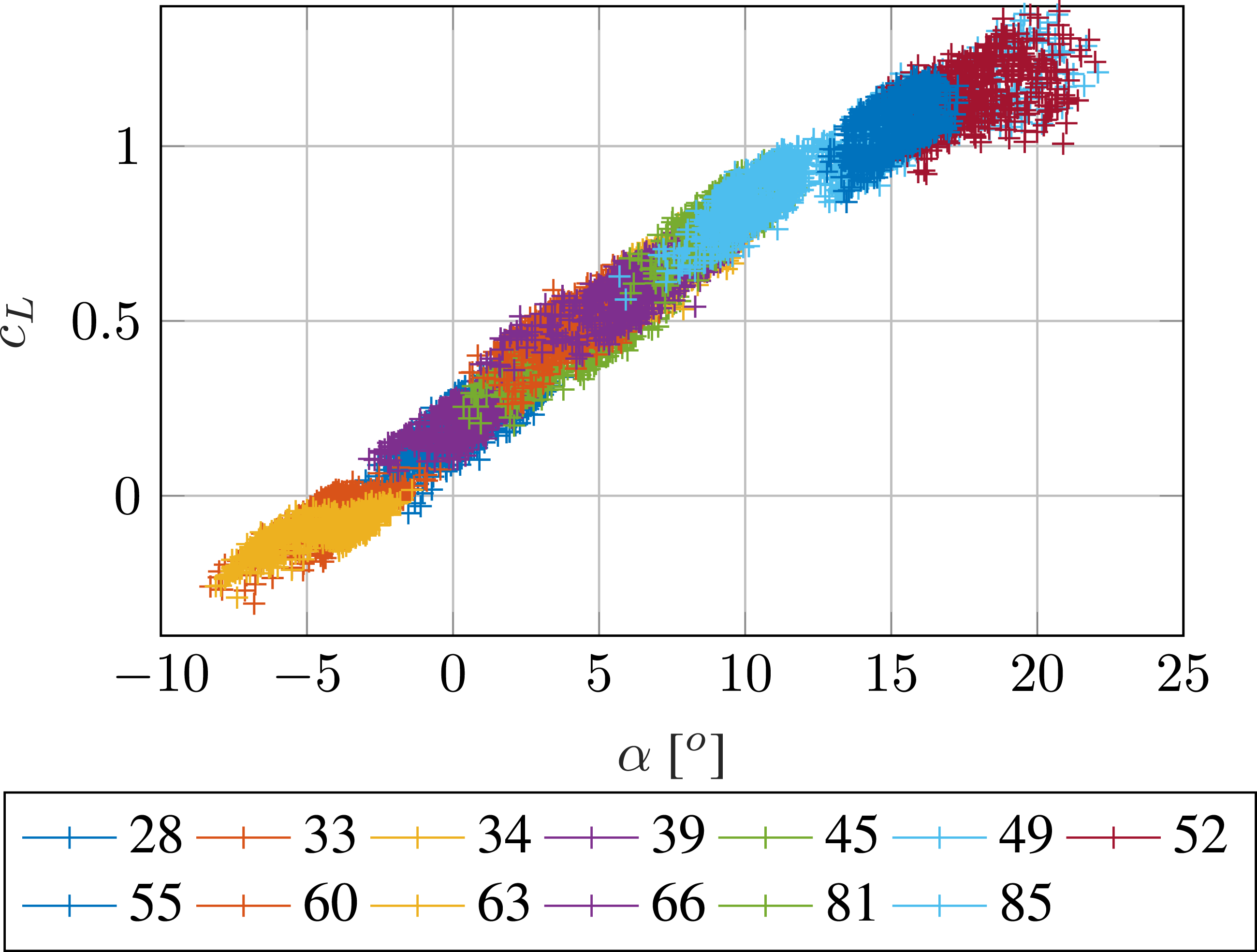
With wind speeds reaching less than 5 m/s during the measurement time in the second week, the inflow speed was dominated by the rotation. At 20 rpm and 10 m radius this results in inflow speeds between 21 m/s with no wind and 21.45 m/s with 5 m/s wind. Hence, the Reynolds number lies around 1.4 ⋅ 106.
To condense these individual c
L
vs. α data pairs into polars, the measured data pairs are clustered into packets with an AoA resolution of Δα = 1
o
. In each of these packets, the c
L
values are averaged providing one point at the polar at the current AoA, for example, all datapoints between α = 0.5
o
and α = 1.5
o
are averaged and displayed at α = 1
o
. Executing this for all flap positions, seven polars can be calculated. These are shown in Figure 12. Measured polars of all investigated flap positions.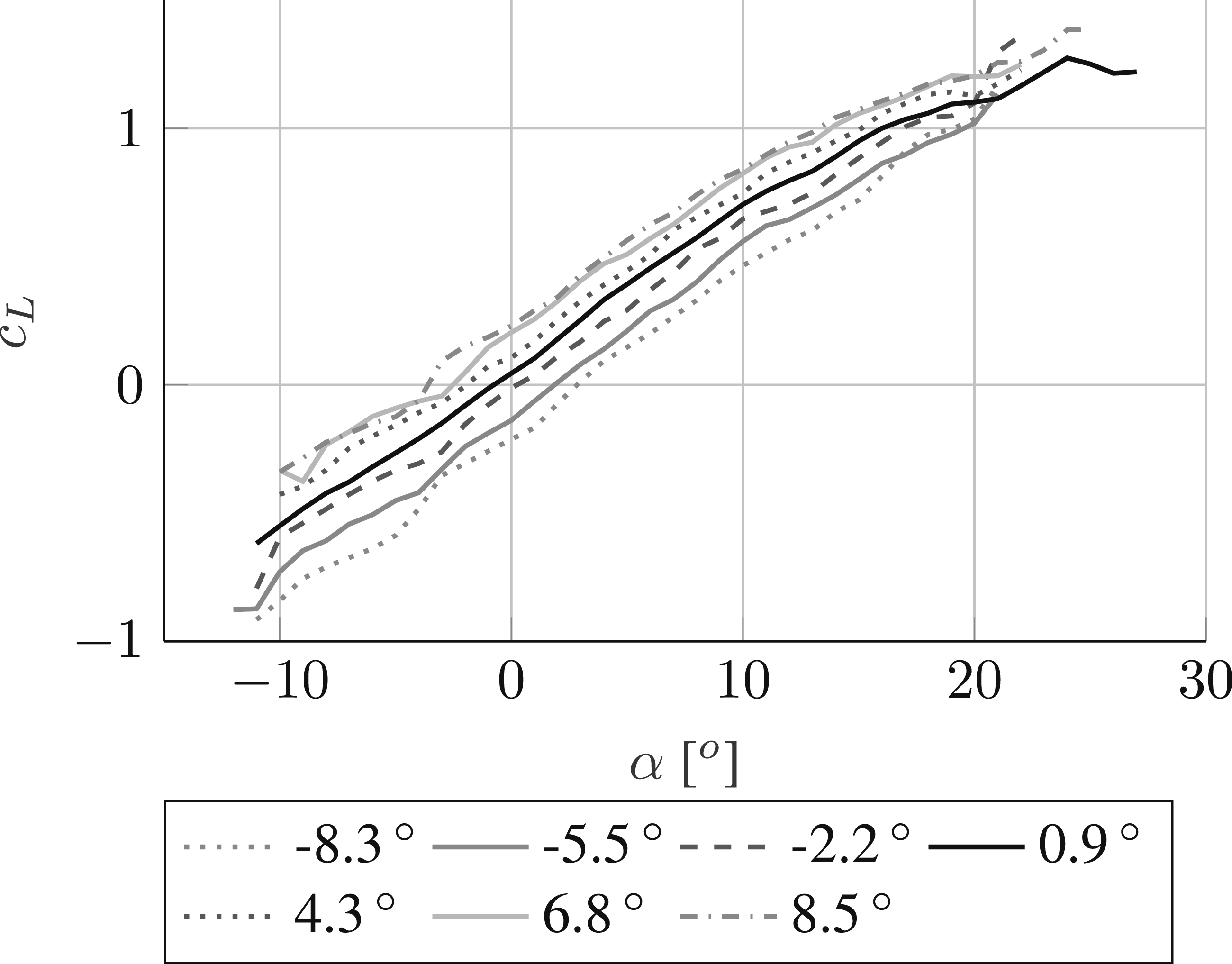
According to the expectation, moving the flap between the measured maximum and minimum positions results in a lift coefficient change of Δc L ≈ 0.45. When looking at the lift slope, it can be calculated to, for example, Δc L /α = 3.76 for a flap angle of β = 0.9 o between α = −5 o and α = 5 o which is significantly less than the theoretical value. Signs of flow separation are not clearly visible even at high α values. A further discussion of these results will be provided in the discussion section of this paper.
Controlled flap movement
After obtaining the flap polars it was intended to investigate the load reduction potential of the flexible trailing edge concept. To achieve this, a controlled flap movement is implemented to counteract the boom bending moment. Since the measurement time was too short to implement complex control algorithms, three simple control methods have been tested: (1) Rotor azimuth control (2) Boom bending moment feedback (3) AoA control
With these three methods the 1/rev movement caused, for example, by the vertical wind gradient is focused. With a rotational speed of 20 rpm, this can be found at 0.33 Hz.
The effectiveness of the control methods is quantified by looking at the flapwise bending moment of the mounting boom of the airfoil section as well as the acceleration in flapwise direction. A set of strain gauges is mounted near the attachment point of the airfoil section. In order to easily compare the bending moment with and without control, a logarithmic dB scale presentation is chosen. In the case of the bending moment M
bf
, the curves are normalized by the highest value in the uncontrolled case as shown in equation (2).
The acceleration is also presented in dB scale with a reference of 1 g as shown in equation (3).
The tests with controlled movement were performed between April 18 and 20. The wind conditions in this time are provided in Figures 31 and 32.
Azimuth control
At first, the flap angle is controlled using the rotor azimuth ψ, which represents the angle of the rotor with respect to the gravitation vector. With each rotation, ψ covers a full revolution of 360
o
. With this, a 1/rev oscillation of the trailing edge and by this a camber change is achieved meaning that differences in lift due to the wind gradient can be mitigated. The flap angle β is set as a sine wave according to equation (4).
Four different phase angles of Δψ = [0 o , 90 o , 180 o , 270 o ] at pitch angles of θ = −7.5 o and θ = 5 o have been investigated to see the different influences on the movement of the demonstrator and the bending moment.
In Figure 13, an exemplary plot of the flap target angle β is provided. It shows the mentioned sine wave with an amplitude of A = 8.5
o
using the full range of the trailing edge flap. Furthermore the measurements were performed in such a way that the control was active for a certain time, after which the controller was deactivated and the flap was positioned in the neutral state. By this an assessment of the effect of the control is possible in a comparable wind situation. Servo target value in azimuth control for Δψ = 180
o
.
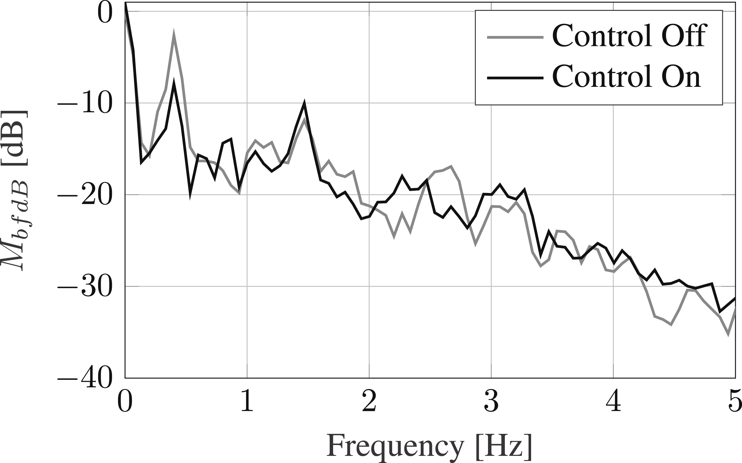
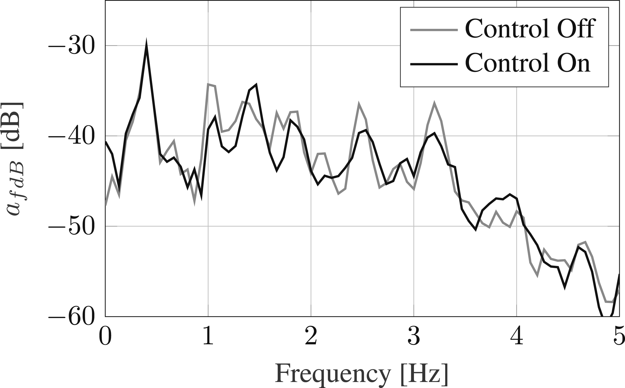
Out of the eight azimuth control measurements, significant reductions as well as increases of the boom bending moment could be demonstrated with different pitch and phase angle settings. Figure 14 shows the boom bending moment spectrum for θ = −7.5
o
pitch and Δψ = 90
o
phase angle where a reduction of 5.3 dB was achieved for the 1/rev movement of the demonstrator at 0.33 Hz. Normalized boom bending moment spectrum for θ = −7.5
o
pitch and Δψ = 90
o
.
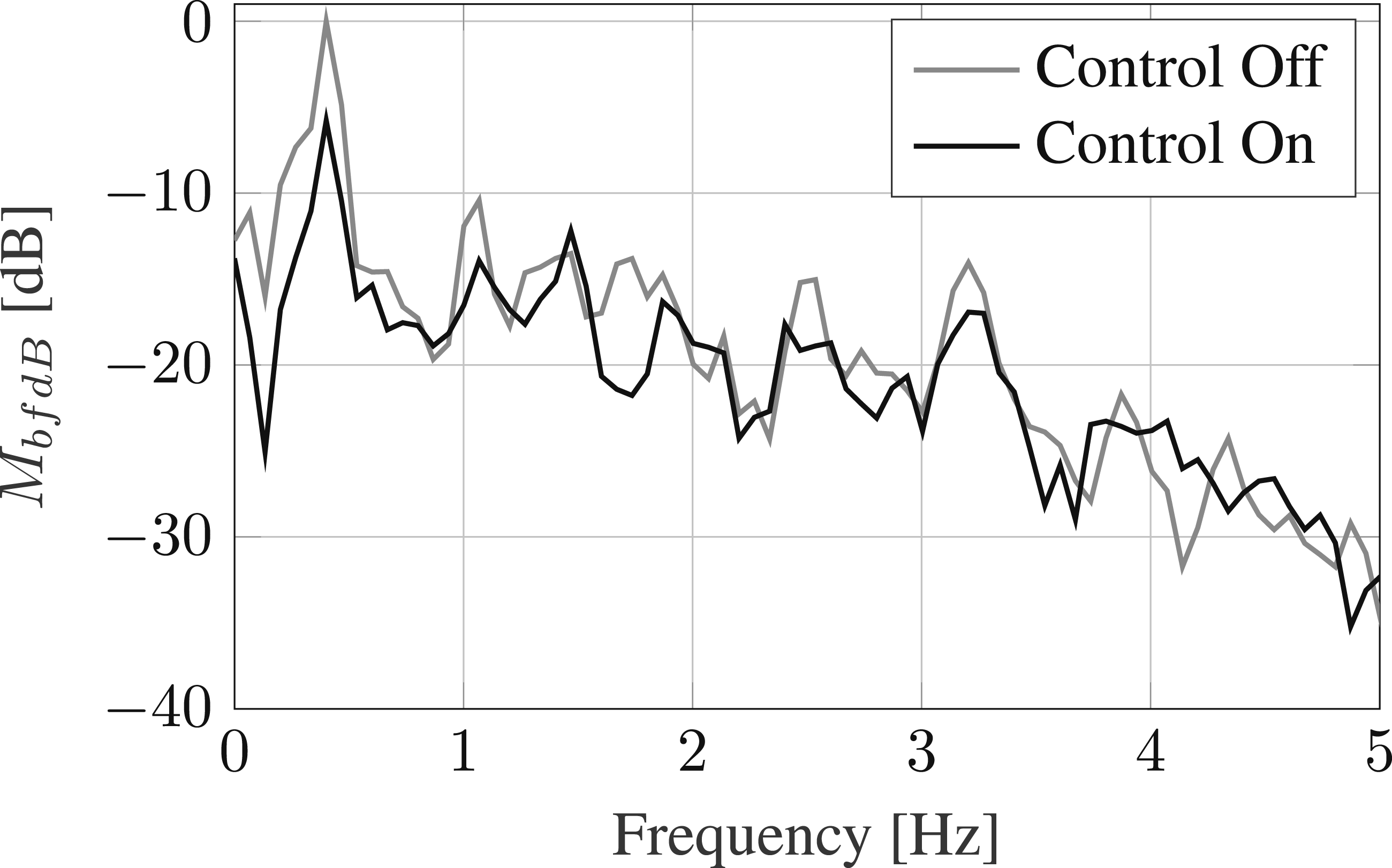
In case of a pitch angle of θ = 5
o
, a phase angle of ψ = 180
o
is required for a reduction of the 1/rev frequency. Figure 15 shows the boom bending moment spectrum of this case. A reduction of 5.8 dB was measured. Normalized boom bending moment spectrum for θ = 5
o
pitch and Δψ = 180
o
.
Besides the boom bending moment also the movement of the demonstrator was measured in the test campaign. Therefore, the signal of one of the accelerometers in the thickness direction of the airfoil is used. Counterintuitive to the expectation, that a reduction of the boom bending moment is correlated to a reduction in the flapwise movement of the demonstrator, the acceleration levels remain constant at the 1/rev frequency independent from the setting of segment pitch angle and azimuth controller phase angle. One example spectrum is given in Figure 16 where the acceleration level is plotted with active and inactive controller. In the spectrum a peak at the 1/rev frequency is clearly visible but there is no difference due to the controller. Besides that, there are some deviations between the spectra of the active and inactive controller at higher frequencies, but due to the fact, that the controller is by design only effective at 0.33 Hz, these are probably caused by stochastic differences in the wind conditions. Acceleration spectrum for θ = 5
o
pitch and Δψ = 180
o
.
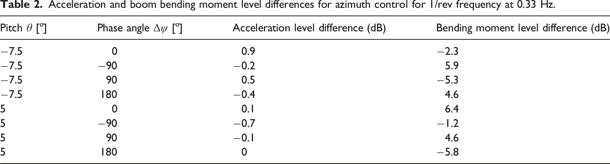
Acceleration and boom bending moment level differences for azimuth control for 1/rev frequency at 0.33 Hz.
Angle of attack control
For a better performance the phase angle needs to be further precised and the flap amplitude also needs to be adjusted to the present wind conditions. One way to achieve this without a complex controller is to use the angle of attack control (AoA control). In this case the flap target value is obtained by multiplying the measured angle of attack α with a constant gain factor B
α
according to equation (5). This would cause the flap to deflect negative if the angle of attack is increased and hence compensate the increase caused by the increased angle of attack. Since the lift varies linearly with the angle of attack and the internal mechanism of the flap was also designed to have a linear correlation between the flap angle and the servo motor angle (see Pohl and Riemenschneider (2023)) the value of B is directly applicable to the servo motors without linearization.
Additionally, a low pass filter at 2 Hz was implemented to adapt the controller to the dynamic capabilities of the flap. Proportional coefficients of the flap angle to AoA ratio of B
α
= −8.5 and B
α
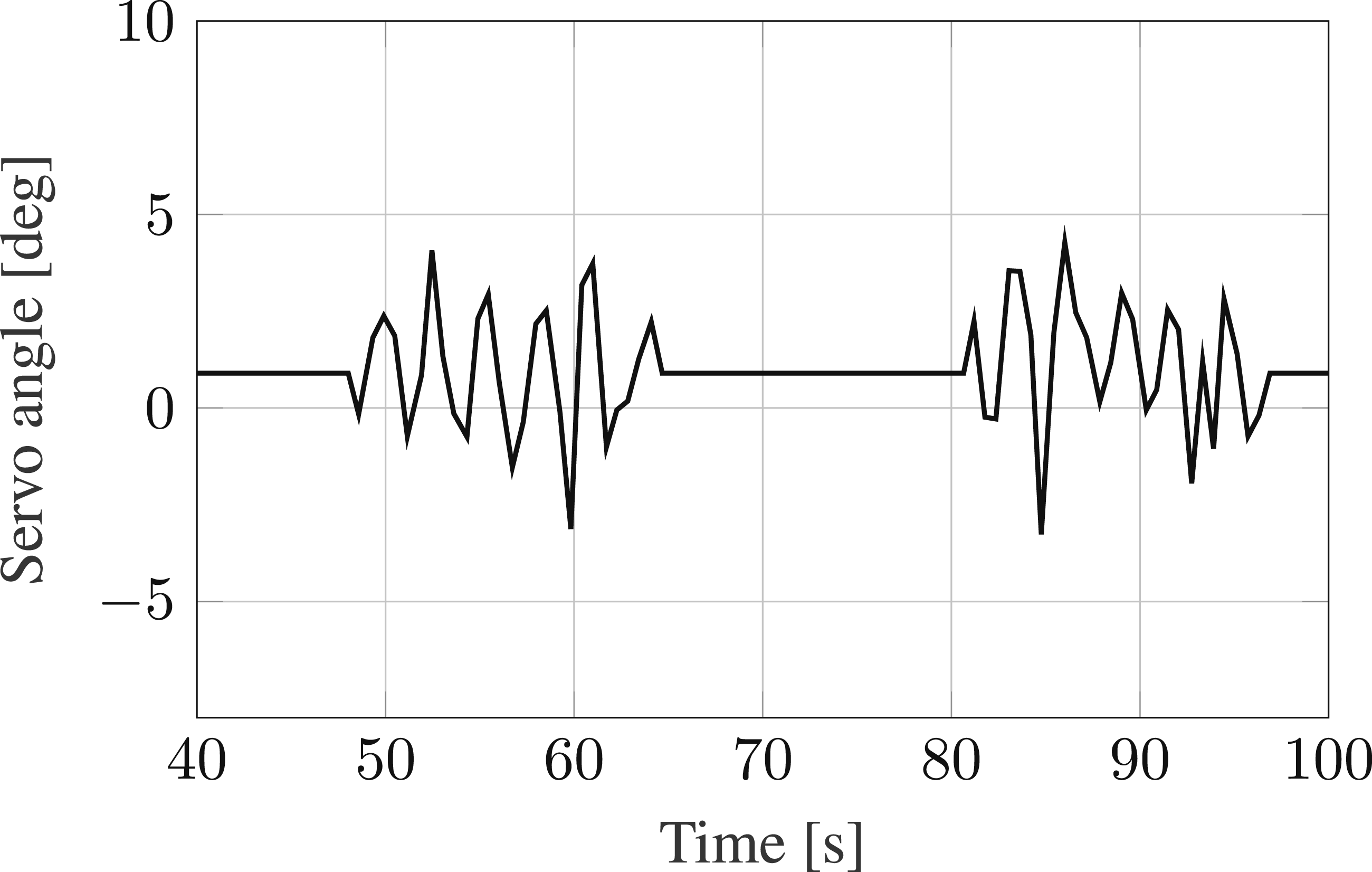
= −12.75 have been investigated where the greater value was found to provide a better result due to the higher flap angles. Figure 17 shows the target value of the flap for an exemplary measurement with Bα = 12.75 and θ = 5
o
. In line with the azimuth measurements, the controller was activated intermittently for 15 s to be able to compare the results in similar wind conditions. Servo target value in angle of attack control for B
α
= 12.75 and θ = 5
o
.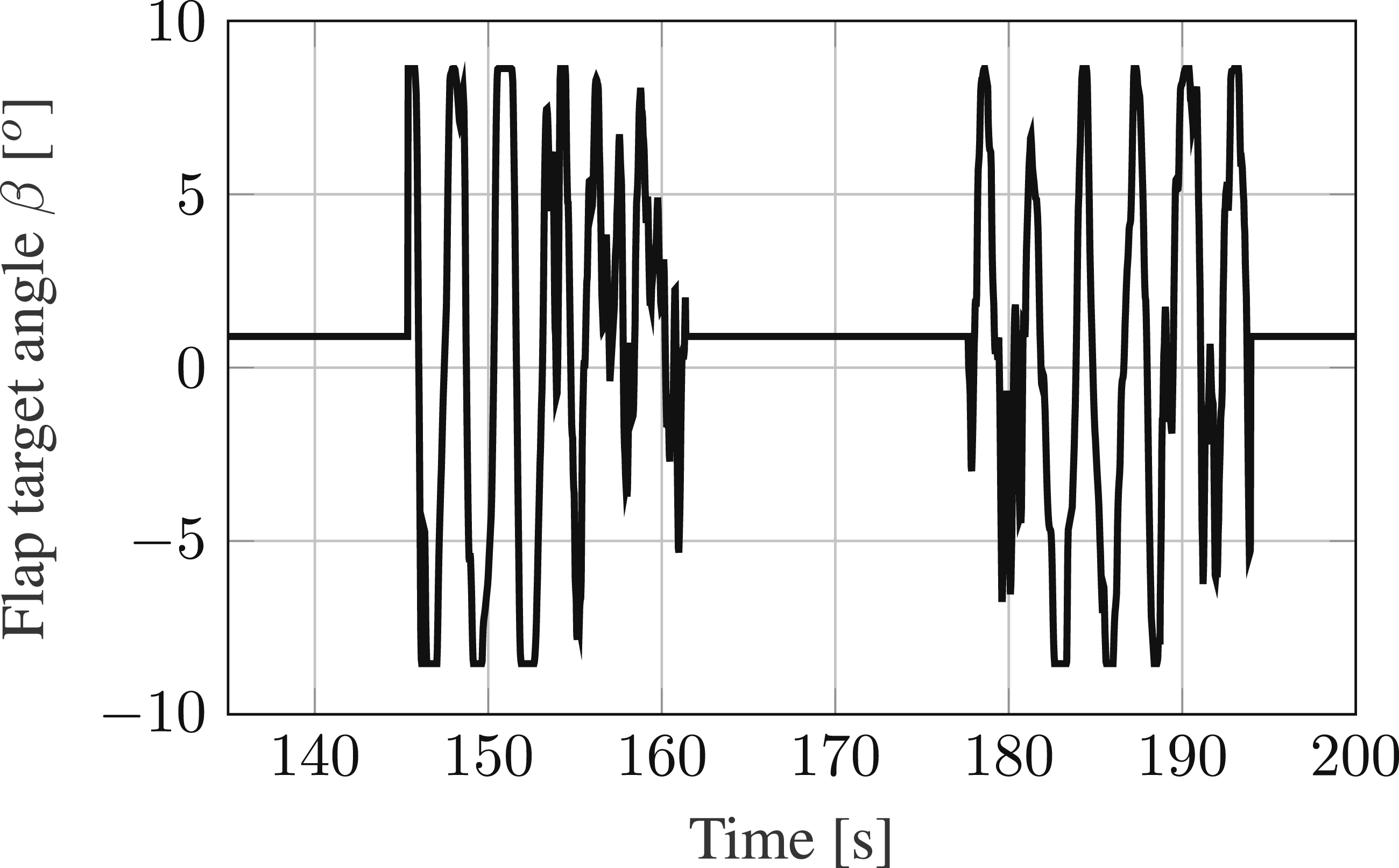
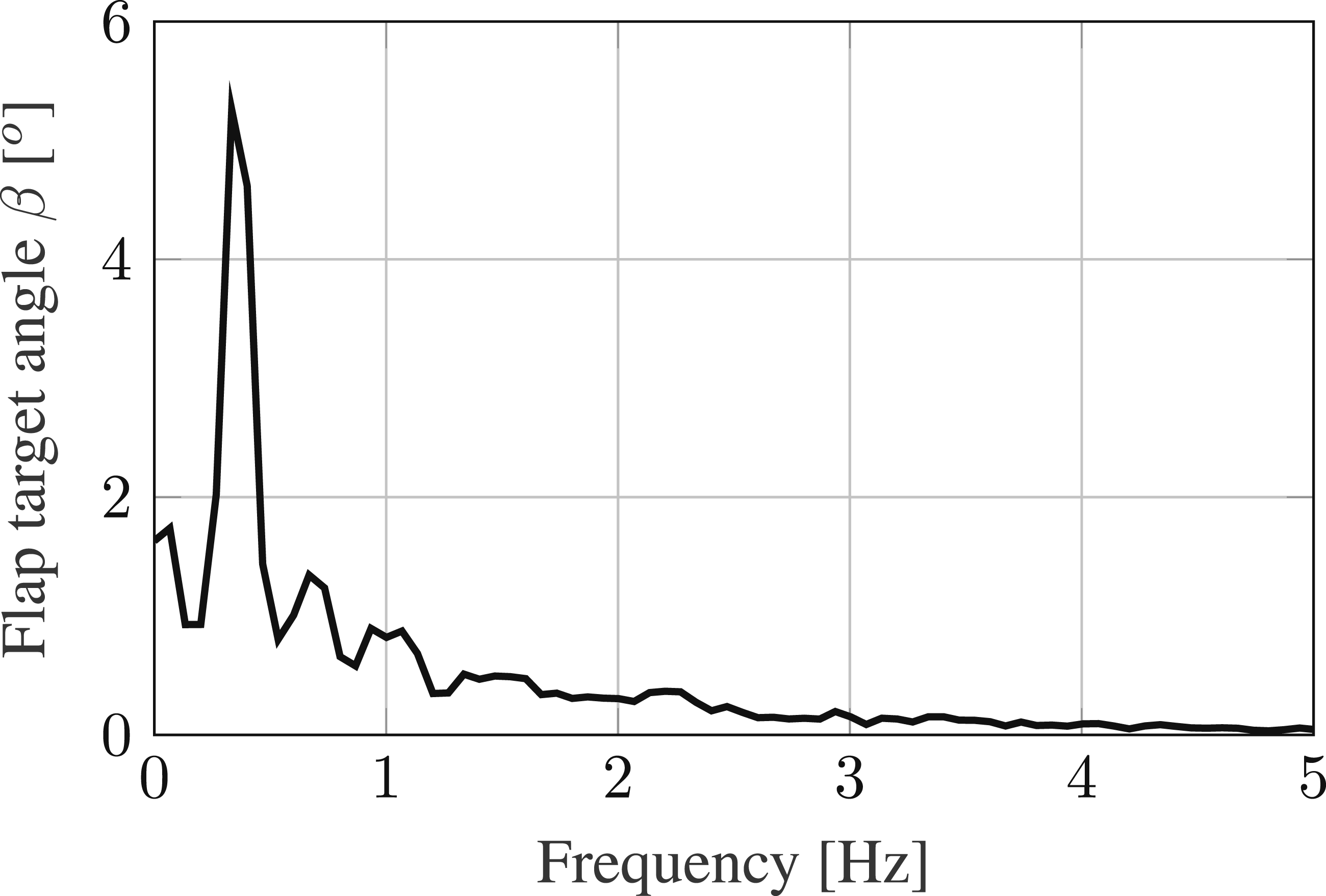
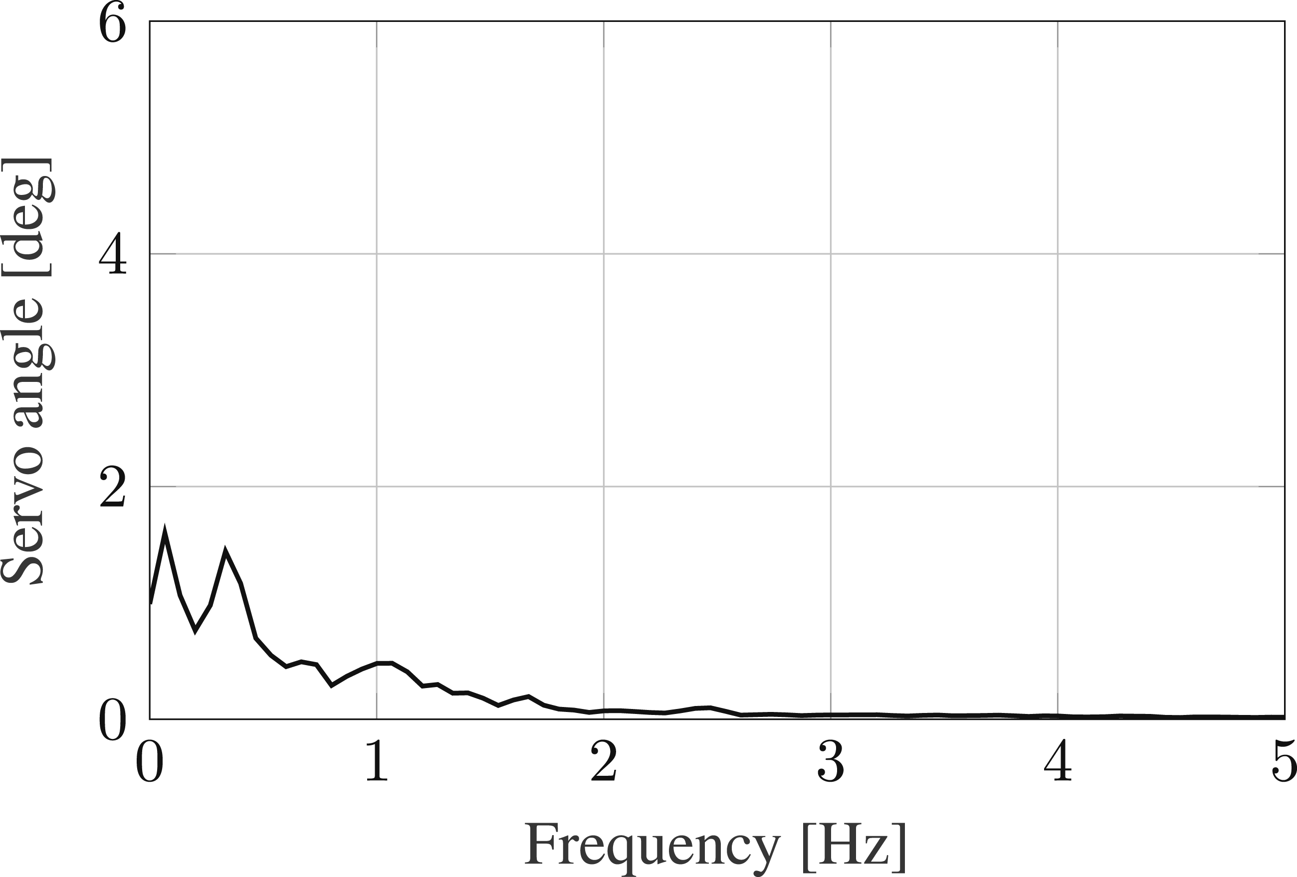
Figure 18 displays the spectrum of the flap target angle. There the 1/rev signal is clearly visible which is caused by the vertical wind gradient. Besides that, a significantly peak is visible at 0.66 Hz which is the second harmonic of the rotation. Due to the dominance of the 1/rev signal, the main effect of the controller is to be expected at this frequency. Servo target value spectrum in angle of attack control for B
α
= 12.75 and θ = 5
o
.
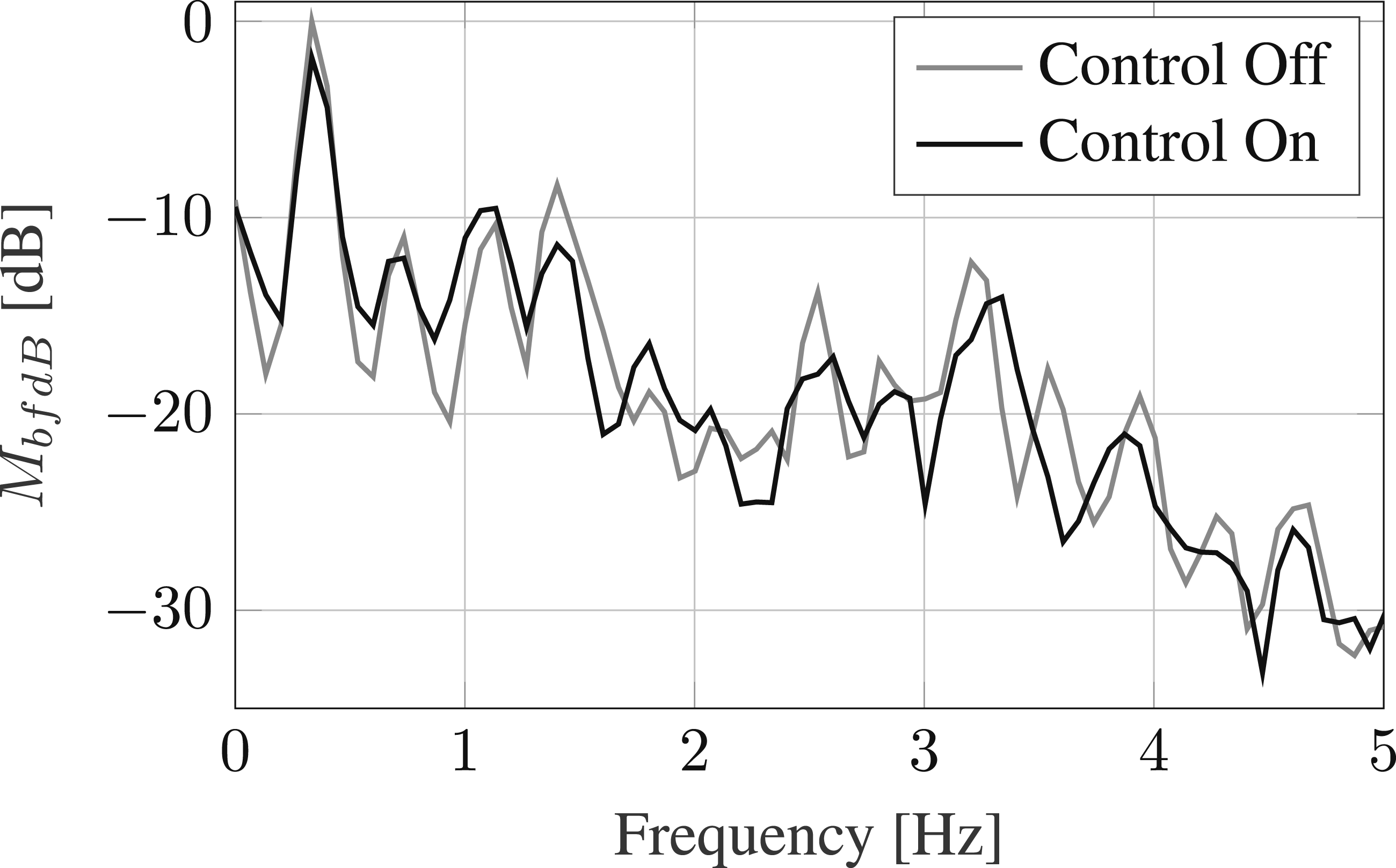
To investigate this, Figure 19 shows the amplitude spectrum of the boom bending moment for the measurement with B
α
= 12.75 and θ = 5
o
. There an amplitude reduction of the 1/rev frequency of 4.4 dB was achieved. Besides that a second amplitude reduction of 4.9 dB is visible at a frequency of 1.4 Hz. Amplitude spectrum of boom bending moment in angle of attack control for B
α
= 12.75 and θ = 5
o
.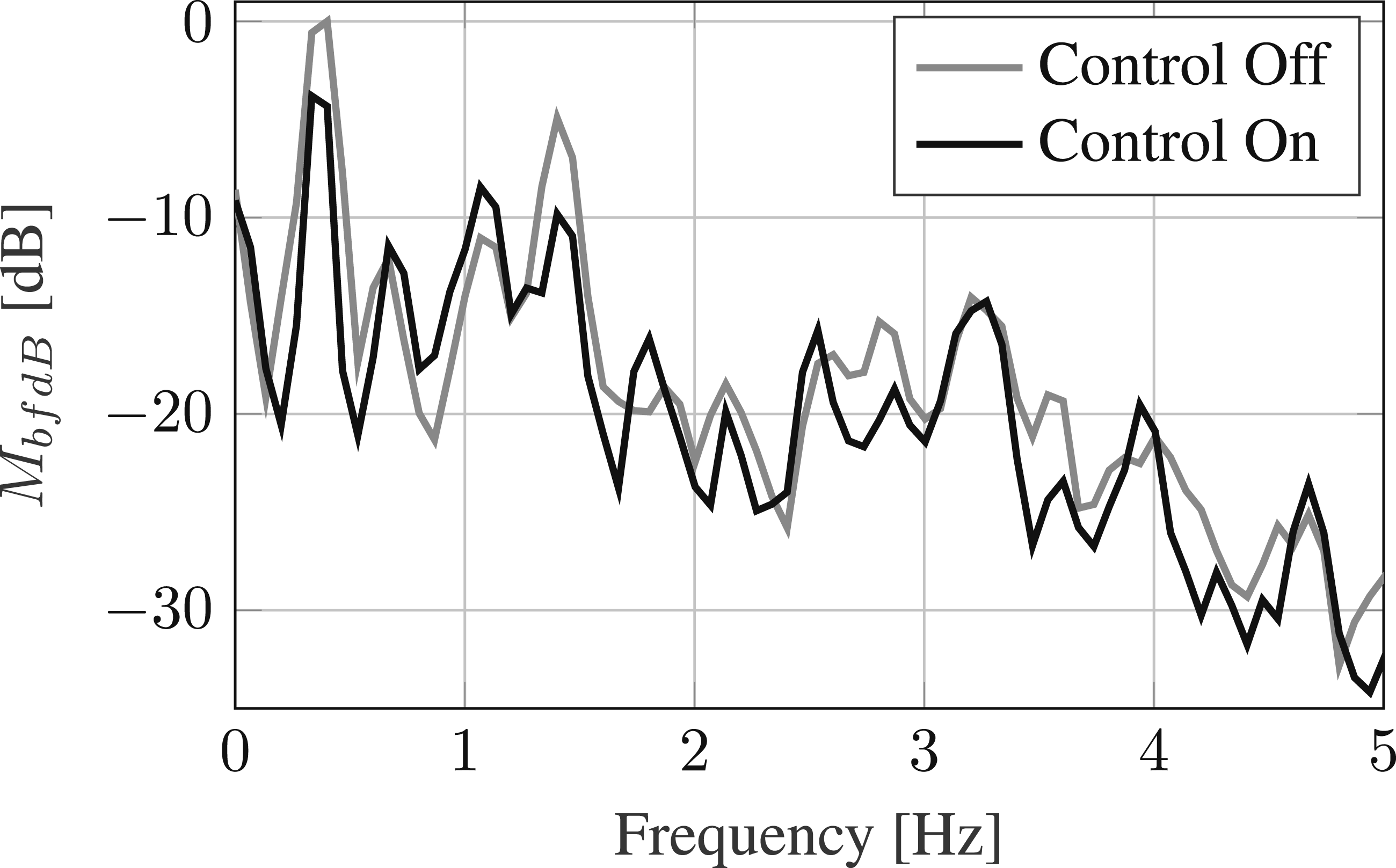
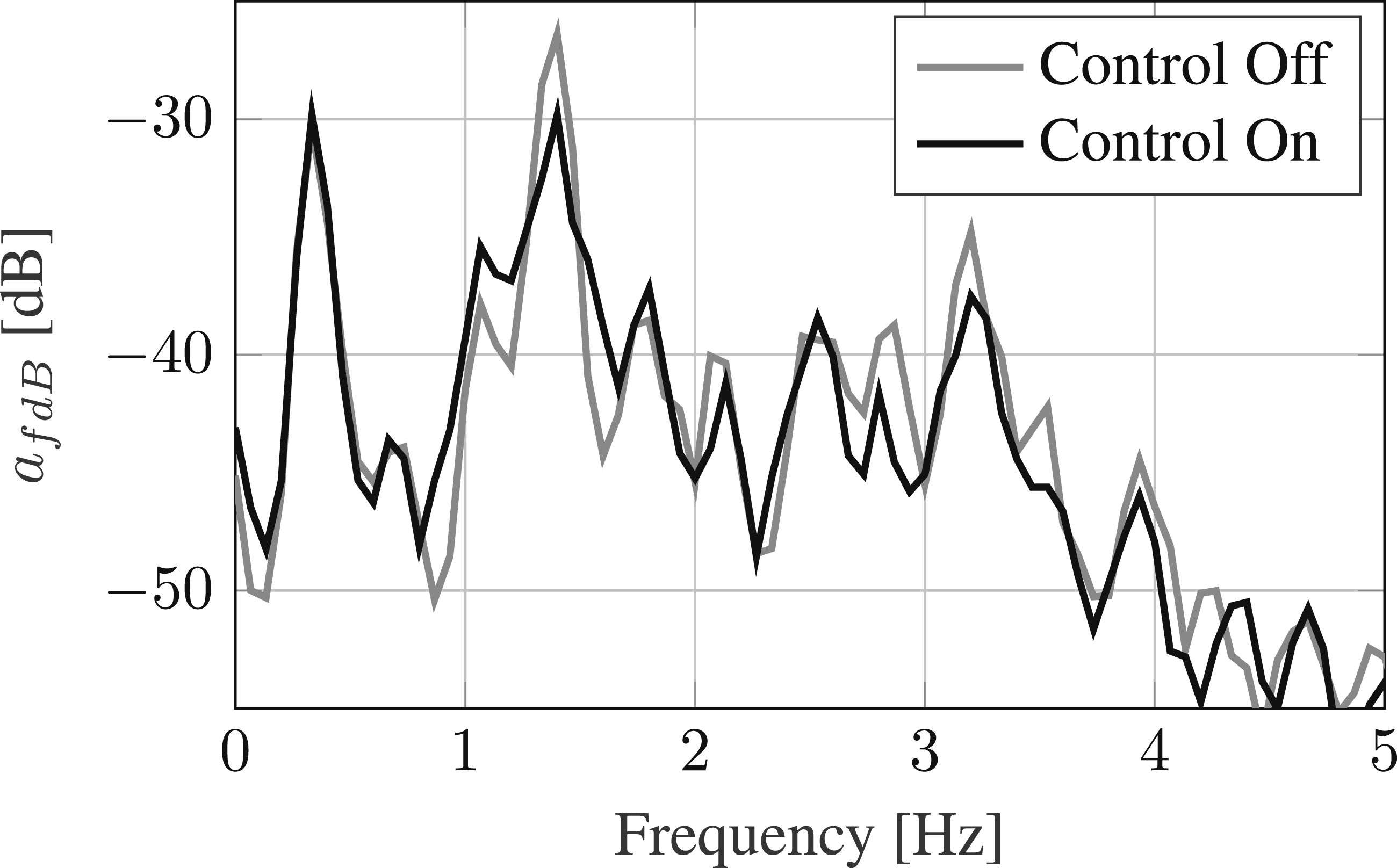
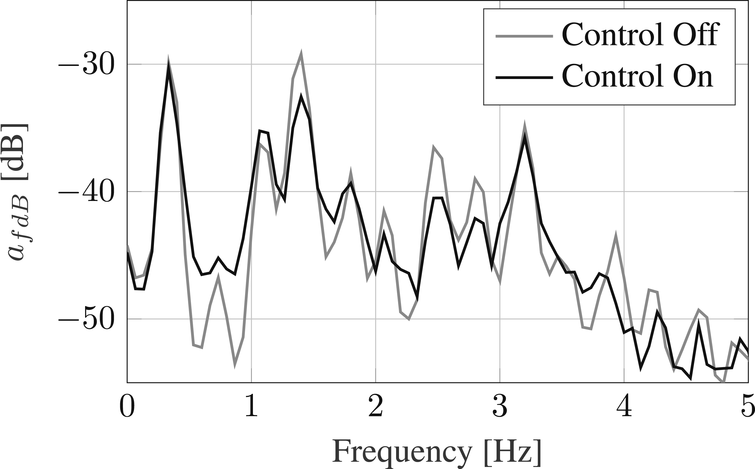
Figure 20 shows the acceleration spectrum for the same measurement. As for the azimuth control, there is no significant amplitude difference at the 1/rev frequency. Interestingly the amplitude reduction at the peak at 1.4 Hz is also visible in the acceleration spectrum with an amplitude difference of 3.4 dB. Amplitude spectrum of acceleration in angle of attack control for B
α
= 12.75 and θ = 5
o
.
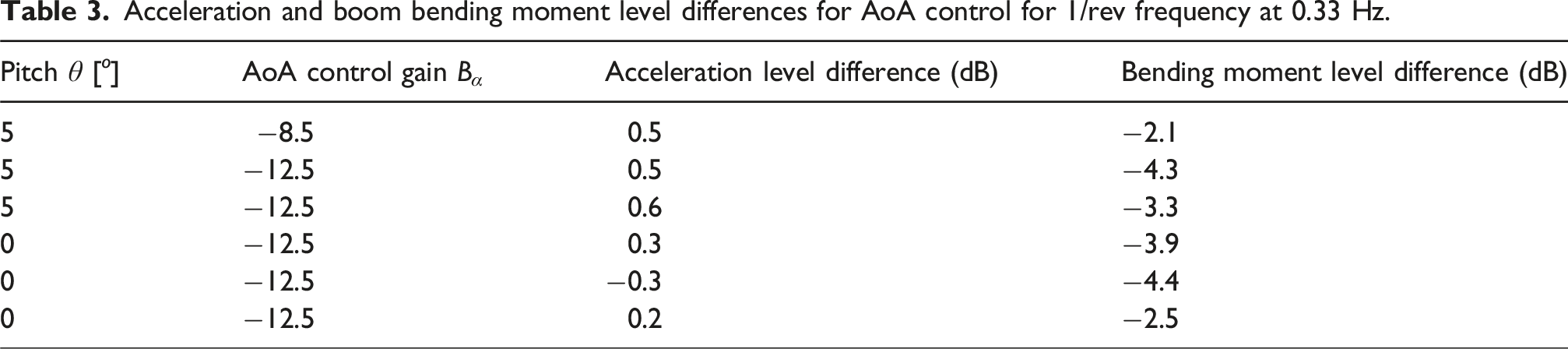
Acceleration and boom bending moment level differences for AoA control for 1/rev frequency at 0.33 Hz.
Acceleration and boom bending moment level differences for AoA control at 1.4 Hz.
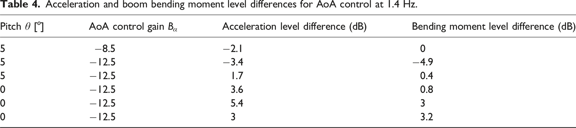
There the measurement shown in Figures 19 and 20 is plotted in the second line. It is the only measurement with significant differences at this frequency so an influence of the controller is unlikely as already assumed. The other measurements even show an increase of the amplitude so this effect is probably caused by differences in the wind conditions.
Bending moment control
As a final step, a direct feedback of the boom bending moment is used as a reference for the flap angle. It also uses a proportional gain B
M
according to equation (6) with the measured voltage of flap bending the strain gauge as argument. Similarly to the AoA feedback a 2 Hz low pass filter is used. Two values for B
M
with opposite sign have been used since the calibration factor and the sign of the strain gauges measuring the bending moment have not been known at the testing time. This is also the reason why no unit for BM can be provided.
Figure 21 shows the flap target angle in bending moment control. Compared to the AoA control, the absolute values are smaller. Servo target value in bending moment control for B
M
= 85 and θ = 5
o
.
This is confirmed in the flap target angle spectrum shown in Figure 22. As expected, the most dominant peak is at the 1/rev frequency and, compared to Figure 18, much smaller. Servo target value spectrum in bending moment control for B
M
= 85 and θ = 5
o
.
With the smaller flap amplitude, the expected boom bending moment reduction should be smaller compared to AoA control. This is proven in Figure 23, where the boom bending moment spectra with and without control are shown. A slight reduction of the 1/rev frequency of 1.8 dB at 0.33 Hz is visible. Amplitude spectrum of boom bending moment in bending moment control for B
M
= 85 and θ = 5
o
.
As for the azimuth and AoA control, no effect on the flapwise acceleration is visible in bending moment control as shown in Figure 24, where the acceleration spectrum is plotted. Amplitude spectrum of acceleration in bending moment control for B
M
= 85 and θ = 5
o
.
Acceleration and boom bending moment level differences for AoA control for 1/rev frequency at 0.33 Hz.
Wind tunnel test
For the wind tunnel tests, a wind tunnel at University of Oldenburg was used. It has a 3 m × 3 m flow nozzle and can operate with an open or closed test section where a maximum flow speed of 42 m/s is achievable with the closed section. This wind tunnel has additionally been added with a variable grid to simulate atmospheric turbulence conditions, (see, e.g., Kröger et al. (2018) or Neuhaus et al. (2020)), but this was not yet operable by the time the tests were done. So the main goal of the wind tunnel tests was to obtain the flap polars for different flap positions. Therefore, the airfoil demonstrator was placed on a turntable to adjust the angle of attack. The outside fairing of the wing was also installed. In addition, a scale is placed between the demonstrator and the turntable to obtain the forces and moments. To exactly control the wind tunnel speed, a pitot tube was placed in front of the airfoil demonstrator. Figure 25 shows the wind tunnel test setup photographed from behind the airfoil. The turntable itself allows 360
o
freedom of rotation. Airfoil test section in wind tunnel, upstream view.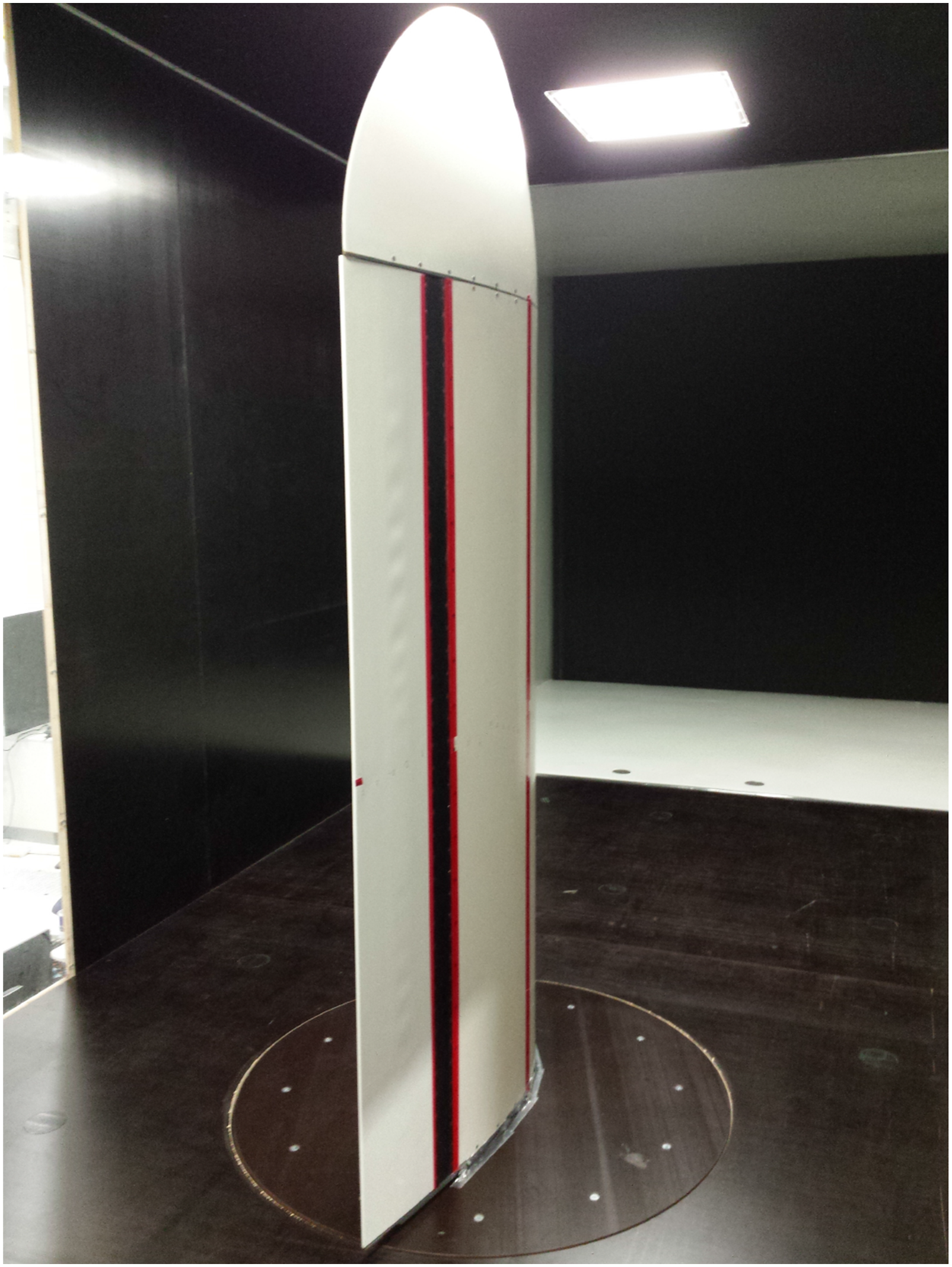
With this setup, flap polars have been obtained for the same seven flap positions, which have already been used in the rotating test. Flow speeds were 10 m/s, 20 m/s and 30 m/s. This yields in Reynolds numbers between Re = 0.67 ⋅ 106 and Re = 2 ⋅ 106. To derive the polars, the wind tunnel scale and the integration of the pressure measurement at the surface pressure taps according to equation (1) have been used. Figure 26 shows the obtained c
L
vs. α polars for all measured flap positions. In the diagram, a flow velocity of 30 m/s was applied and the elastomer covers were used, which have been rebuilt before the wind tunnel tests as mentioned above. Note that the polars based on the scale show the measured lift force divided by the dynamic pressure and a wing surface of 2 m2 without any further postprocessing to compensate the finite wing length and the fairing. Measured polars for all trailing edge positions at 30 m/s with elastomer cover based on wind tunnel scale.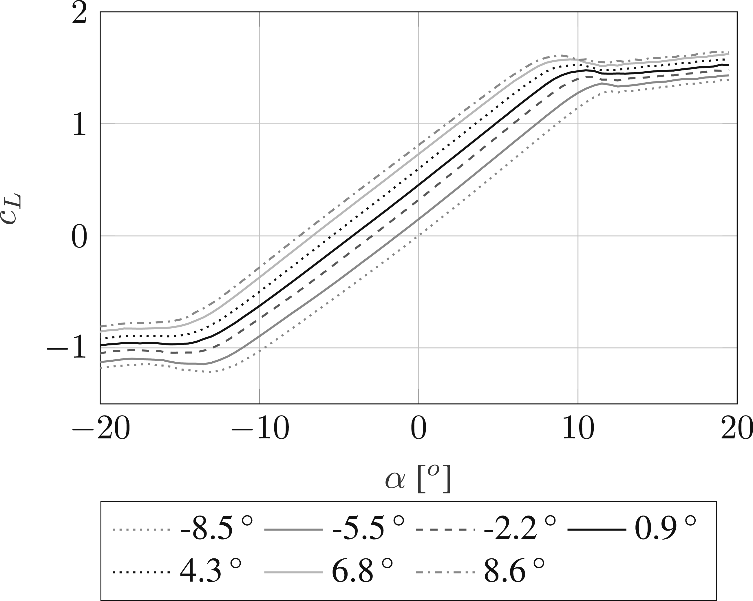
In the figure, it can be seen that a deflection of the trailing edge clearly results in a change in lift coefficient. This is in line with the measurements that have been obtained in the rotating test. For comparison, Figure 27 shows the same polars obtained with the pressure taps. In general they show the same behavior but the maximum c
L
is slightly smaller. Presumably this is an effect caused by the infinite wing and the fairing at the end of the wing, where the lift polar cannot be directly measured without postprocessing. With this in mind, it seems the fairing and the gap at the end of the wing are nearly canceling each other. Measured polars for all trailing edge positions at 30 m/s with elastomer cover based on surface pressure taps.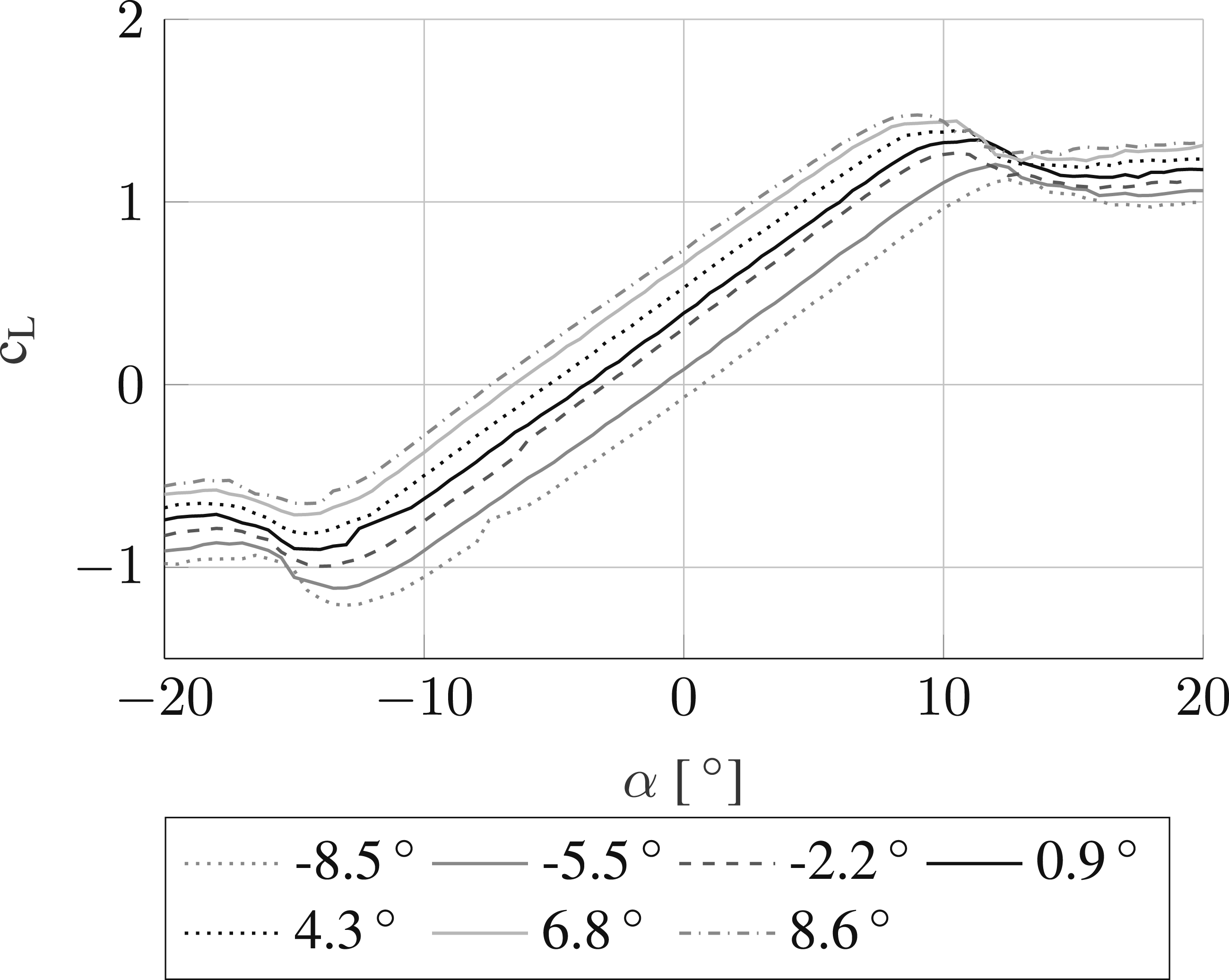
As a last step, a comparison between the elastomer covers of the gap constituting the aerodynamic surface from the rear spar of the airfoil section to the flexible trailing edge and the sliding cover is done in the wind tunnel. This will also allow conclusions on the rotating test rig measurements, which have only been made with the sliding covers. Figure 28 shows the polar comparison of both covers for a speed of 30 m/s for three flap positions measured with the wind tunnel scale. Obviously the differences between both cover concepts are minuscule. Measured polars for three different trailing edge settings with elastomer (E) and gliding (G) cover at 30 m/s.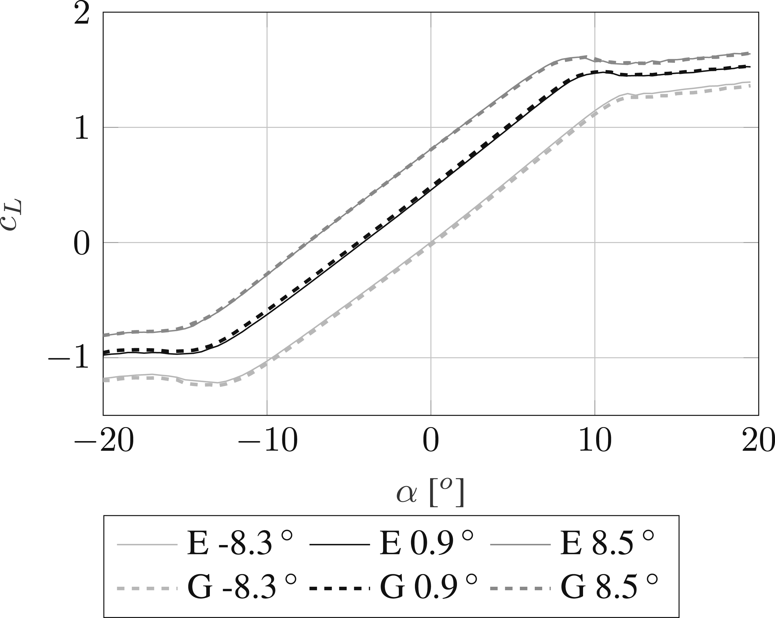
In the Appendix, the polars are also included for 10 m/s and 20 m/s. Interestingly, the lift coefficients of the pressure tap measurements for 10 m/s are significantly below the measurements based on the wind tunnel scale. Furthermore the obtained polars based on the pressure taps are noisy compared to scale measurements. The probable reason therefore is the low surface pressures at the low wind speeds where the pressure sensors are operating at their lower limit. Angle of attack deviations or flow separations can safely be excluded as an explanation since this would also affect the maximum angle of attack of the linear part of the c L curve as well as the wind tunnel scale data. A further explanation including XFOIL simulations of the airfoils can be found in the Appendix.
As already mentioned above, all these data show the raw measurements without any corrections for the limited span of the test airfoil section. In addition, a full 360 o polar is plotted in Figures 35 and 36. In the central region, the linear part of the polar can be found. Outside of this, the lift coefficient exceeds the maximum lift. This is explained by the wind tunnel blockage, since the airfoil demonstrator covers more than 2 m2 of the 9 m2 test section.
Discussion
In general, the expectations in the active, flexible trailing edge have been fulfilled. The change of lift could be demonstrated both in the wind tunnel and in the rotating test. Also a reduction of bending moments with a controlled deflection of the trailing edge was proven in the rotation test.
In contrast to the wind tunnel measurements presented in Figure 26, the polars of the rotation test in Figure 12 show less lift slope and do not show signs of flow separation in comparable angles of attack. To further investigate this, Figure 29 contains the polars of the wind tunnel and rotation experiment in comparison to data obtained in TU Delft wind tunnel Llorente et al. (2014) for the clean DU91-W2-250 airfoil. The Reynolds numbers are Re = 1.4 ⋅ 106 for the rotation test, Re = 2 ⋅ 106 for the wind tunnel test and Re = 3 ⋅ 106 for the data from Llorente et al. (2014). Measured polars at wind tunnel test Oldenburg, rotation test at DTU compared to data from TU Delft.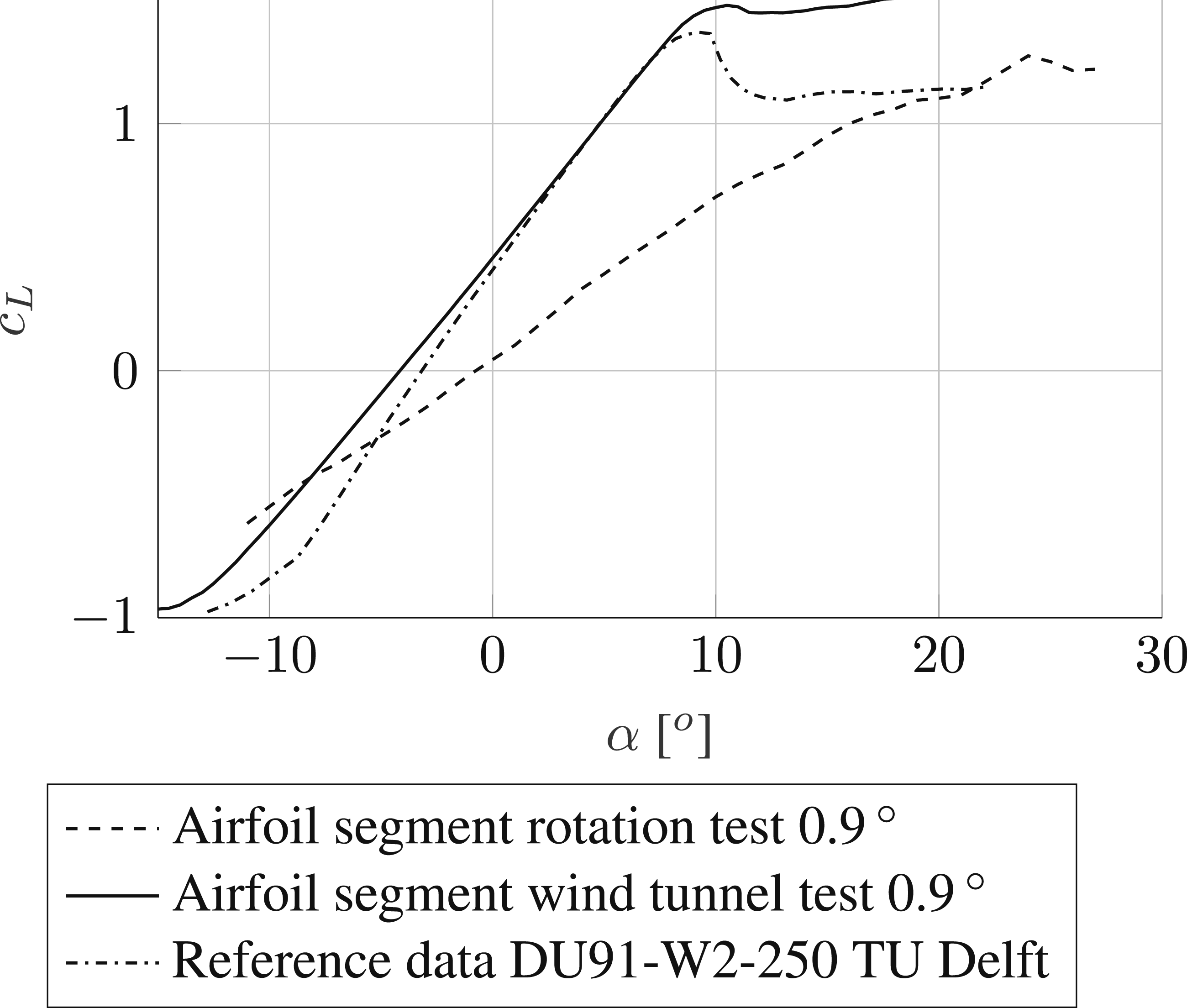
There a small slope deviation is visible between the test in Oldenburg and the data from Llorente et al. (2014). The bigger deviation occurs in the rotating test. The probable reason therefore arises from the finite span and low aspect ratio of the demonstrator. In the wind tunnel test in Oldenburg, a gap of
The limited span and low aspect ratio effect also appears to be the reason for the lack of stall signs in the flap polar obtained by the rotation test. Due to the low aspect ratio the wing tip vortices are comparably strong which influences the flow on the whole airfoil. Since the author does not have access to 3D CFD, no further investigation of this effect is possible.
When looking at the measurements with a controlled movement of the trailing edge, it can be stated, that all used control schemes—azimuth control, angle of attack control and bending moment control—are able to reduce the amplitude of the bending moment in the mounting boom of the segment. For the sake of an easy implementation only proportional controllers have been used in the tests and there was not enough measurement time to fully tune the controller gains of each method. Therefore, the presented results, where an amplitude reduction was possible with even these simple algorithms, can be seen as a lower estimate of the potential of a load control with the flexible trailing edge.
Comparing the results of all tree control approaches the azimuth has shown the greatest reduction of the boom bending moment, followed by the AoA control and lastly the bending moment control. When considering this, it has to be taken into account, that the measurement time at site was not sufficient to perform a detailed design of the control algorithms to derive the optimal gains for all control methods. For this reason, these results cannot be used to assess the control methods among each other. As an example increasing the feedback gain of the bending moment controller may have increased the performance.
A common outcome of all measured control strategies is the different effect of control on the segment movement and the boom bending moment at the 1/rev frequency. The controller clearly has an effect on the bending moment since variations of the control gain produce a corresponding effect on the bending moment. However, differences in the flapwise acceleration amplitude remain minuscule. This observation may be explained by two effects simultaneously occurring on the acceleration signal. First, the 1/rev frequency is well below the first eigenfrequency of the boom and segment demonstrator in flapwise direction. Therefore, no resonance is enhancing the displacement and a movement of the airfoil is only caused by bending the mounting boom. Due to the stiffness of said boom, the acceleration amplitude based on the movement of the segment is small. Therefore, also the difference of the acceleration caused by controlling the trailing edge has a very low absolute value. Second and probably dominant is the fact that the acceleration signals in all directions at the 1/rev frequency are the sum of movements due to aerodynamic forces and the rotating gravity acceleration in the segment coordinate system. This is also present in the flapwise direction acceleration regarded in this paper if it is not exactly perpendicular to the gravity vector. Thus, slight misalignments will cause a cross sensitivity of gravity on the flapwise acceleration covering the acceleration caused by movement. Removing the part of gravity is only possible when the spatial orientation is precisely known. Since these data have not been recorded in the experiments with the required precision, a further evaluation of the acceleration in terms of control effectiveness at the 1/rev frequency is not possible.
Additionally, there are some cases where the amplitude of the controlled case is higher than the amplitude of the uncontrolled case as, for example, in Figure 19 at 1 Hz. This is most likely not an effect of the controller since the control signal at this frequency is very low as shown in Figure 18. Instead, this is probably a consequence of turbulences in the inflow.
Conclusion and outlook
With the flexible trailing edge demonstrator wind tunnel and rotating tests have been performed in order to investigate the influence of the flap on the aerodynamic behavior. Within the wind tunnel and the rotating tests, a change in the lift coefficient due to a deflection of the trailing edge could be demonstrated. Additionally, the rotating test was used to investigate a controlled movement of the trailing edge in order to reduce the flapwise loads. Therefore, three proportional controllers were set up, which use the rotor azimuth, the angle of attack or the bending moment in the mounting boom as a reference. It could be shown, that all three control schemes are capable of reducing the flapwise bending moment in the mounting in a magnitude of up to 5 dB. Since there was not enough time to optimize the parameters of each control scheme, the obtained results have to be seen as a lower estimate of their potential. For these reasons, it can be concluded that the flexible trailing edge is a suitable concept for load reduction of wind energy blades.
Maturing the trailing edge for an active load control of wind turbines requires the investigation of different aspects of the current design. First, the design algorithm and models have to be adjusted to real rotor blades with spanwise variable geometry due to twist, prebending, and blade sweep. This also incorporates higher fidelity aerodynamics to adapt the structure to the occurring loads and to define the actuation needs for the trailing edge. Second, the actuation method has to be matched with the requirements of wind energy, that is, for lightning resistance, actuation speeds and maintainability in wind turbines. Third, fatigue has also to be focused in the further development concerning the fiber composite part of the trailing edge, the driving mechanism and especially the elastomer covers since maintenance is expensive.
With these aspects in mind, the next logical step consists in an experimental campaign at a real wind turbine with a blade modified with a custom made trailing edge. Then comparing the loads between the modified blade with an unmodified blade directly allows to assess the effectiveness of the trailing edge and the used controller. Operating the system for an extended time period also allows to discover and estimate fatigue and wear effects.
Footnotes
Author contribution
Martin Pohl: Design and testing of the flexible trailing edge, data analysis, and paper writing.
Johannes Riemenschneider: Project management and organization, and paper proofreading.
Funding
This work was funded by the Federal Ministry for Economic Affairs and Climate Action on decision of the German Bundestag in the frame of the SmartBlades2 project (funding reference no. 0324032A-H).
Declaration of conflicting interests
The authors declare no potential conflicts of interest with respect to the research, authorship, and/or publication of this article.
Data Availability Statement
Measurement data from the tests are available via the author upon reasonable request.