Sage Journals: Discover world-class research

Abstract

Small-scale H-Darrieus turbine (HDT) often struggles to reach self-sustained power producing speed due to low start-up torque. Low torque is sometimes manifested in the form of torque plateau or ‘dead band’. To improve torque development, turbine design variables such as blade chord-to-radius ratio (c/r) and solidity (σ) play critical role. To understand the effect of c/r only, this study analyses turbines with identical σ but different c/r using unsteady computational fluid dynamics (CFD). Results show that larger c/r enhances torque by influencing the leading-edge flow and vortex formation and convection. Two mechanisms are identified: (i) amplification of the variation of incidence angle along blade chord, effectively acting as aerofoil-camber morphing, and (ii) high blade pitch rate effect, especially at low λ (<1) where intra-cycle pitching is significant. These findings highlight the sensitivity of torque generation to c/r, offering design guidance for improving HDT start-up performance.

Keywords

dead band H-Darrieus turbine NACA0021 self-start start-up vertical axis turbine

Introduction

H-Darrieus turbine (HDT) is mechanically simple device, making it suitable as small-scale hydrokinetic renewable power generation, particularly in off-grid areas (Kirke 2020, 2024). However, its limited self-starting capability without external power source or auxiliary control systems remains a persistent issue in practical deployments (Kirke and Lazauskas 2011).

Despite their construction simplicity, the orbital motion of the blade(s) creates a highly complex unsteady flow field. This leads to significant intra-cycle and inter-cycle torque variations during the transient start-up phase. The start-up process of HDTs typically comprises several distinct stages as seen in terms of rotational speed versus time diagram (Asr et al., 2016; Celik et al., 2020; Hill et al., 2009; Mohamed et al., 2021; Worasinchai et al., 2016). As shown in Figure 1(a), the turbine undergoes variable acceleration during start-up. These variations can be categorised into four primary stages: (I) initial acceleration, (II) low acceleration with a plateau, (III) rapid acceleration, and (IV) decreasing acceleration.

Figure 1.

(a) Typical start-up 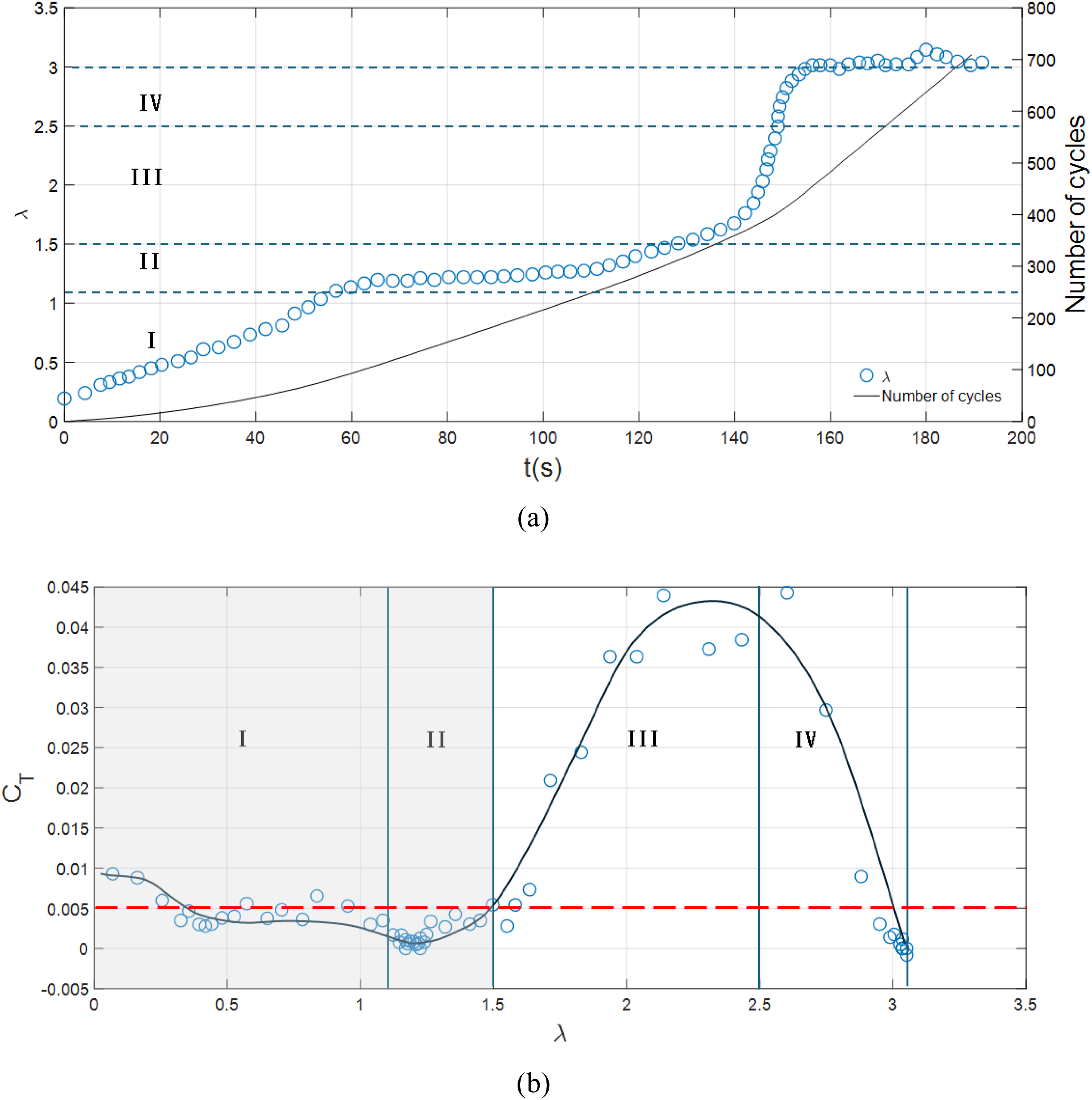$λ - t$ of unloaded H-Darrieus cross-flow turbine (Hill et al., 2009). The stages are initial acceleration stage (I), low acceleration with plateau stage (II), rapid acceleration stage (III) and deceleration stage (IV). (b) Corresponding $T - λ$ expressed in non-dimensional coefficient of torque. Note the shaded region is where torque plateau occurs. The dashed line in the torque–speed diagram represents a hypothetical parasitic torque of a system. Average intra-cycle torque would need to be above this line across all λ for the rotor to be self-starting.

Stage I begins with a positive net torque that accelerates the turbine from rest. In Stage II, torque decreases significantly, resulting in low acceleration. At this point, the turbine may become trapped in a torque plateau. Turbines that can self-start advance to Stage III, where acceleration increases rapidly. In Stage IV, acceleration slows as the turbine approaches its steady-state unloaded rotational speed. For water turbines, this corresponds to a tip-speed ratio (λ) between 3 and 4. Although several definitions of self-start exist, there is no consensus on a precise definition (Ebert and Wood 1997). In this study, a turbine is considered self-starting if, under steady freestream flow and unloaded condition, it progresses through all start-up stages and reaches Stage IV, achieving a tip-speed ratio of approximately 3 or higher. Stage IV represents a stable operating condition where the turbine maintains self-sustaining speed, even under varying load or freestream conditions.

By taking the derivative of the transient rotational speed profile, instantaneous torque variation with tip-speed ratio can be estimated as illustrated in Figure 1(b). This figure clearly demonstrates the existence of torque plateau. Although in this case the turbine appears to overcome the plateau, a rotor with torque greater-than, but in close proximity to the parasitic torque line is vulnerable to becoming trapped at the plateau. The parasitic torque increase (environmental or otherwise e.g. bearing fouling) – for the rotor of the reference (Hill et al., 2009) there appears to have been negligible parasitic torque, though the turbine required a substantial number of revolutions (exceeding 300) to transition through stages I and II owing to low net torque in these stages. Low-solidity wind and hydrokinetic turbines operating under low speed condition is particularly susceptible to this problem. Experimentally the existence of dead band is shown in water turbine (Polagye et al., 2019). However, as shown in CFD simulations, at higher flow velocities, the increase in angle of attack elevate drag forces and consequently generate higher torque, thereby mitigating the dip enabling the turbine to escape this stalling condition (Maalouly et al., 2022).

Addressing the start-up issue requires improving rotor torque in the region where λ < 1. Several passive and actives approaches have been proposed. Passive approaches are often preferred because they simplify manufacturing, maintenance, and operation. In contrast, active methods involve multiple moving parts, complex mechanisms, and external power sources. In the λ < 1 region, torque enhancement depends on the interplay between lift and drag. For passive methods, this becomes a matter of balancing aerofoil performance – either by improving lift or drag. Aerofoils with suitable aerodynamic characteristics across the full 0–360° incidence range, under both static and dynamic conditions, are desirable. Research on aerofoils generally falls into three areas: symmetrical profiles with varying Reynolds numbers and thickness (Du 2016) and cambered (Bianchini et al., 2015), and the effects of pitching dynamics (Holst et al., 2019). When applied to HDT rotors, symmetrical aerofoils such as NACA0015, NACA0018, NACA0022, and NACA0024, and cambered aerofoils like NACA2418, exhibit different start-up behaviours. Of these, only NACA0018 and NACA2418 have been used on rotors that progressed unaided through the torque plateau stage. And a rotor with NACA2418 reached steady tip speed in less time (Asr et al., 2016).

Passive approaches to HDT modification include changes to symmetrical aerofoils, such as cut-outs (Celik et al., 2022) and slots (Abdolahifar and Karimian 2022). A notable example is the J-blade, a cut-out design that improves rotor torque when the cut-out is placed on the outer surface (Celik et al., 2022). This improvement results from changes in the flow field around the blade. Slotted blades also enhance performance by maintaining flow attachment for a larger portion of each revolution. Blade number further influences start-up behaviour (Dominy et al., 2007). Keeping solidity constant while changing blade number requires proportional adjustments in chord length, assuming rotor radius remains fixed. These changes affect aerofoil aerodynamics and torque during start-up. This is shown by Sun et al. (2022) where the lower number of blades turbine had higher acceleration from rest.

Another passive approach is the use of helical-bladed turbines. These turbines generally self-start more easily than H-Darrieus turbines of comparable blade number and size. However, they tend to reduce the coefficient of performance (Sun et al., 2022). In the reported experiments, the absence of a Stage II torque plateau may be attributed to the high solidity of 0.76.

To overcome the issue of low torque at the start-up phases, multi-rotor configurations have been investigated (Bhuyan and Biswas 2014; Hosseini and Goudarzi 2019). These designs use a secondary co-axial rotor to provide additional positive torque. Typically, the secondary rotor is of the drag type, such as Savonius (Bhuyan and Biswas 2014) or Bach (Hosseini and Goudarzi 2019) variants. However, adding a secondary rotor increases overall solidity, which reduces performance at the operating tip-speed ratio.

Active approaches focus on improving start-up through active blade pitching and blade morphing. Active pitch-control methods dynamically adjust blade angles to achieve target incidence angles (Kong et al., 2024; Le Fouest and Mulleners 2024; Sagharichi et al., 2016). Another active approach involves energising the boundary layers including synthetic jets (Botero et al., 2022) and plasma actuators (Zare Chavoshi and Ebrahimi 2022, 2024; Zhu et al., 2019). Readers are referred to review on active flow control on wind turbine blades (Saemian and Bergada 2025). These actuators are mainly positioned at blade leading-edge; hence, they are most effective when the leading-edge faces the relative flow. For HDT blades, this is beneficial when λ > 1, where the incidence angle is below 90°.

Another factor influencing start-up is rotor moment of inertia. The time required to reach free-spin steady state depends on this parameter (Arab et al., 2017; Celik et al., 2020; Liu et al., 2016; Tigabu et al., 2022). While moment of inertia directly affects the transient behaviour the time to reach steady state and the rotational speed fluctuation, it does not influence the cycle-averaged steady-state rotational speed.

Due to the orbital motion of the blade, the incidence angle varies along the chord and the variation is strongly dependent on c/r and the location of mounting point (Migliore et al., 1980). Mounting point is the strut-blade connection point. By considering only the blade orbital motion, that is, zero freestream velocity, blades with c/r = 0.114 and 0.260 with mounting point at quarter chord are shown to experience positive shift of angle of attack (incidence angle) by 1.6° and 3.7°, respectively. As the angle of attack increases, the blade is expected to experience premature blade stall. However, if the mounting point is at or beyond mid-chord, the shift becomes negligible or even negative. Thus, increasing c/r can delay stall. For large c/r values, the effective leading-edge incidence angle decreases significantly (Keisar et al. 2020, 2024). Under these conditions, flow remains attached to the blade surface for a longer portion of each revolution. This suggests that c/r could play a role in improving torque generation during start-up.

While virtual cambering has been known as discussed above. The potential positive effect of blade orbital motion on rotor torque in continuous cambering “virtual morphing” of the blade, has not been adequately discussed. The present work aims to gain deeper insight of the effect of virtual morphing on the self-starting performance specifically on torque plateau (dip) mitigation of a three-blade turbine and a one-blade turbine with the same radius and same solidity. The results indicate that for a given solidity, σ (in this case 0.128) there is dependency of the C_T - λ (Torque – rotational speed) profile on c/r. Comparison of coefficient of performance, C_p and Coefficient of torque, C_T are obtained and explained by analysis of the flow field around virtually morphing rotor blades.

Computational fluid dynamics procedure

Governing equations and turbulence model

To obtain torque – rotational speed profile of HDT, one could use the Double Multiple Streamtube model (Mannion et al., 2020). With this method, dynamic lift and drag characteristics of the blades must be available given the blades on the Darrieus rotor undergoing continuously changing angle of attack (Worasinchai, 2012; Worasinchai et al., 2016). When such data is not available, Double Multiple Streamtube model with dynamic stall correction or approximation have been used (Bangga et al., 2019; Masson et al., 1998). Another way is to solve the unsteady Reynolds-Averaged Navier-Stokes (RANS) equations using Computational Fluid Dynamics (CFD) to simulate the interaction of the flow around a rotating turbine at constant rotational speed. At each of the rotational speeds, the rotor torque (which varies on an intra-cycle basis) over a few rotational cycles can then be averaged.

A two-dimensional (2D) CFD approach is commonly used to study HDT (Alaimo et al., 2015; Balduzzi et al., 2014; Castelli et al., 2011; Maître et al., 2013; Mohamed et al., 2021; Rezaeiha et al., 2018). However, 2D CFD is shown to overpredict coefficient of performance. This is associated to the three-dimensional effects such as induced velocity, blade tip loss and spanwise flow (Hao et al., 2026). To address this limitation, addition of mass and momentum sources terms into 2D CFD model has been proposed (Hao et al., 2026). In the present work, 2D CFD is adopted to reduce the computational cost while still producing useful insight of instantaneous coefficient of performance and flow field information (Maître et al., 2013). The compressible Reynolds-averaged Navier-Stokes (RANS) $k - ω$ Shear-Stress Transport (SST) $k - ω$ model was chosen as it effectively blends both the formulation of the $k - ω$ model and the $k - ε$ model such that the SST model can switch between the two formulations to satisfy the turbulent boundary layer flow and far-field undulated eddies (ANSYS 2023). It is also well adapted to the strong adverse pressure gradients which occur in and around turbine blades. This model has been reported in a number of journal articles and publications (Balduzzi et al., 2014; Maître et al., 2013).

The pressure-based solver was used for all simulations as water is fundamentally incompressible. Fluent^® provides several solution Pressure-Velocity coupling solver schemes which include SIMPLE, SIMPLEC, PISO and coupled. The first three solve the momentum and pressure correction equations separately. The Coupled solves them simultaneously within each iteration. The velocity, pressure, and temperature fields are coupled together in the equations, and they are solved together in a tightly coupled manner. By solving the equations together, the Coupled solver can consider the feedback between the velocity and pressure fields more accurately, resulting in a more robust and efficient convergence compared to the Simple solver. However, the computational cost of the Coupled solver is generally higher. The SIMPLE method is relatively computationally efficient and stable for many practical applications but may require more iterations to converge, especially for complex flows. In this study, ANSYS^® Fluent^® CFD code was adopted.

The SIMPLE algorithm has been adopted for this study with suitably fine time step as detailed in the time-step set-up section. The comparative study between SIMPLE and coupled scheme was carried out. The coefficient of torques of the two coincides confirming the suitability of the SIMPLE scheme with suitably fine time-step size. The process (Rezaeiha et al., 2018) taken to ensure the result is independent of the azimuthal increment of the rotor per time step, domain size, and total time (or total number of rotations) is explained.

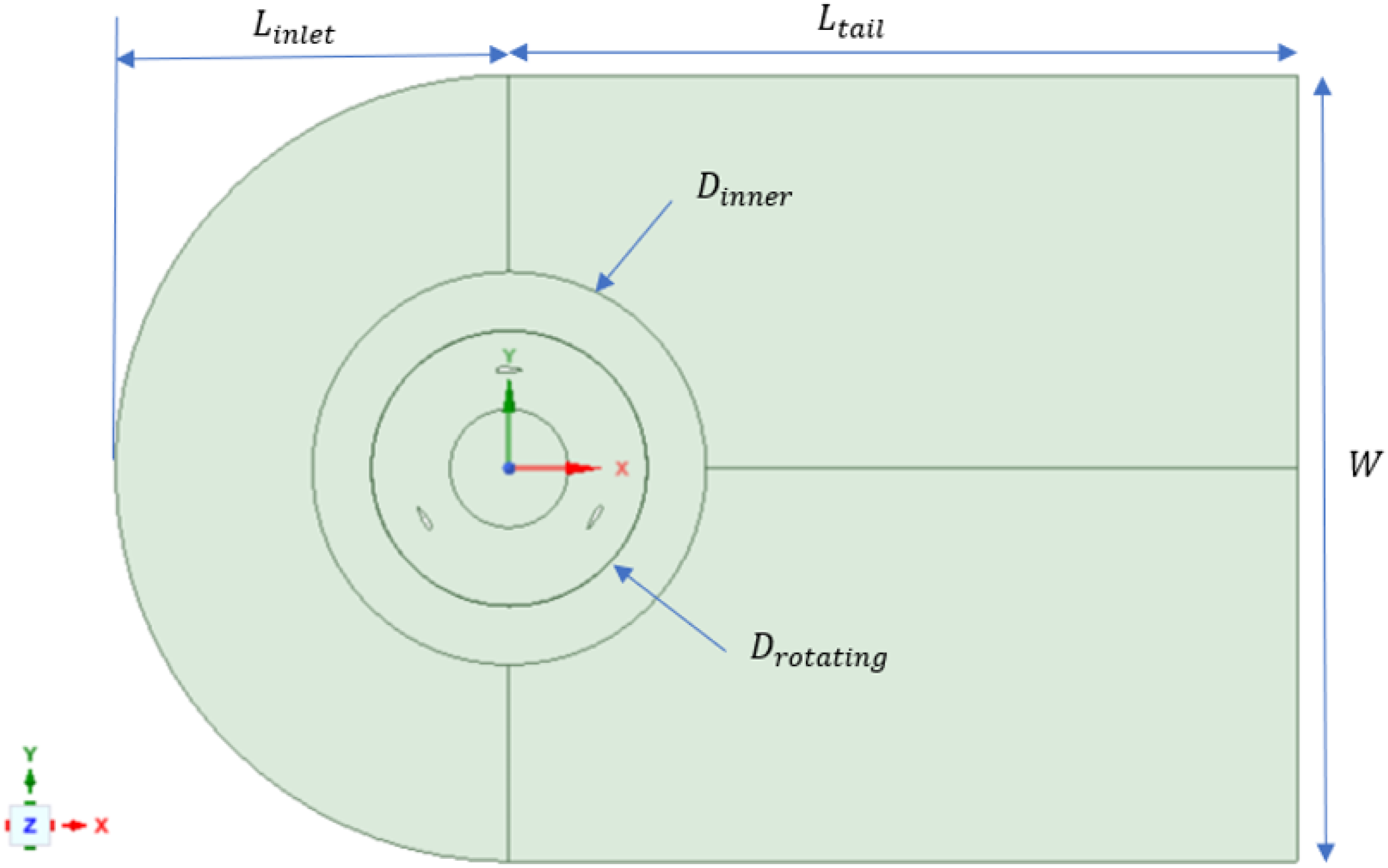
The geometry of H-Darrieus turbine and the simulation domain size

The geometric characteristics of the NACA0021 aerofoil and the turbine are summarised in Table 1. The blade chord length c and the turbine diameter D served as the baseline scales on which the overall dimensions of the CFD domains were sized. The domain size is an important part of the geometry set up. Several studies on HDT have previously used domains which are substantially larger than the turbine diameter in an effort to reduce influencing effects of the boundary conditions on the flow around the turbine toward negligible levels, these domains typically ranging in length from 60 to 120 times larger than the turbine diameter (Alaimo et al., 2015; Mohamed et al., 2021). Additionally, a large downstream space of 120D to 140D enables analyses of the associated distribution, pressure and velocity fields, and decay characteristics of the wake, given the extra domain length allows a high degree of recovery of the downstream flow toward freestream conditions following the mixing and turbulence that results from the interaction between the flow and the rotor. The detailed research into the critical issues in the CFD simulation of H-Darrius wind turbine was adapted and used to verify the domain independence (Balduzzi et al., 2014). Accordingly, the fluid region was set to a ratio of the turbine diameter such that ratio between inlet (

L_{i n l e t})

and outlet (

L_{t a i l})

, domain length (L) and width (W) are prescribed as follow and shown in Figure 2.

(\frac{L_{t a i l}}{L_{i n l e t}}) = 2

(1)

(\frac{L}{D}) = \frac{L_{i n l e t} + L_{t a i l}}{D}

(2)

Table 1.

NACA0021 aerofoil and turbine dimensions and parameters.

Configuration	Three-Blade	Single-Blade
Aerofoil	NACA0021	NACA0021
Chord (c)	67 mm	201 mm
Diameter, (D)	500 mm	500 mm
Number of blades (N)	3	1
Solidity $(σ = \frac{N c}{π D})$	0.128	0.128

Figure 2.

2D 3-Blade HDT with NACA0021 aerofoil profile. Chord length 67 mm, radius = 250 mm. Not to scale.

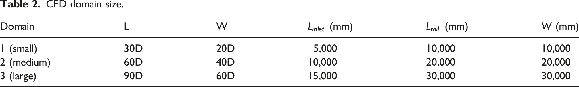
The model was tested at three domain sizes as detailed in Table 2 to assess the influence of the proximity of the boundaries – note, however, that the shortest of the domains ‘Domain small’ is considered herein to be of sufficient downstream length as to be compatible with the typical length of wake observed for Darrieus-type rotors, as seen, for example, in Peng et al. (2021). The turbine is placed within rotating domain with diameter, D_rotating = 1.25D. Additionally, several Bodies of Influence (BOI) shown in Figure 3 were created to segment the fluid domain as part of the mesh sizing methodology. The BOI enclosing the rotating domain diameter, D_inner = 1.75D.

Table 2.

CFD domain size.

Domain	L	W	$L_{i n l e t}$ (mm)	$L_{t a i l}$ (mm)	$W$ (mm)
1 (small)	30D	20D	5,000	10,000	10,000
2 (medium)	60D	40D	10,000	20,000	20,000
3 (large)	90D	60D	15,000	30,000	30,000

Figure 3.

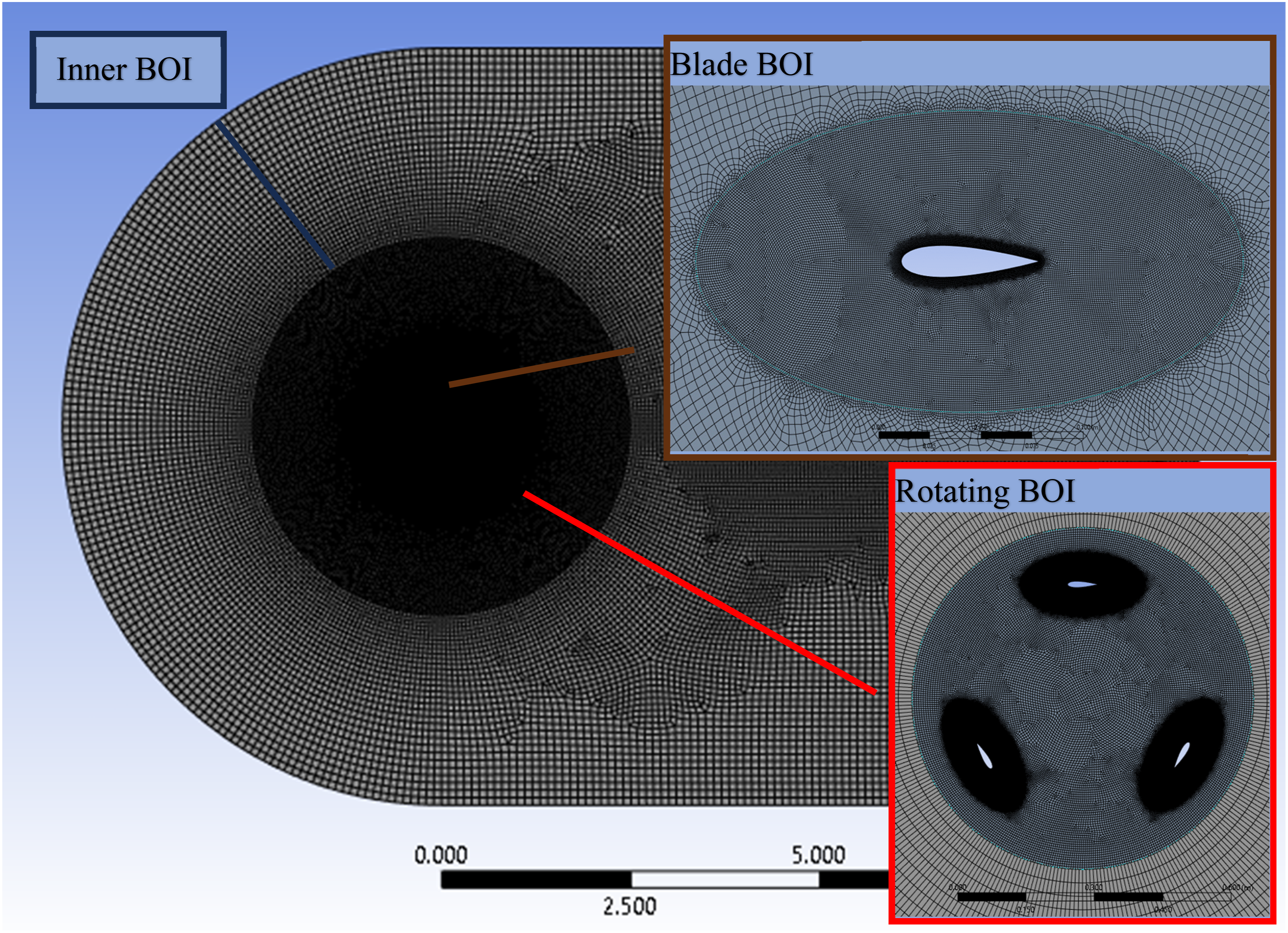
NACA0021 3-Blade HDT mesh geometry and set-up.

To ensure that the fluid flow for each domain was fully developed, each domain was run for a minimum flow time such that a fluid particle initially at the inlet then passed through the full length of the domain. Additionally, a rotor-loading convergence criterion was adopted such that five revolutions were required in which the difference in average torque of successive revolutions was less than 1%. When this condition was met, the average coefficient of torque was taken to be the average across the last five rotor revolutions, and this was used for comparison between the three domain sizes. A comparison of the coefficients of torque for all three domains concluded that as the domain was increased in size the coefficient of torque and power converged as in Balduzzi et al. (2014). Due to the large number of CFD simulations required in the present study, a balance between computational time and precision and accuracy of the CFD estimate of the rotor torque had to be accepted. Therefore, the medium domain was selected.

The inlet boundary was set as a velocity inlet, U_inlet = 1 m/s. The blade surfaces were treated as non-slip wall, while the far-field top and bottom boundaries were assigned a no-shear condition to eliminate the influence from domain boundaries. The outlet boundary was set to Absolute Backflow with zero-gauge pressure. Backflow Pressure was selected to Total Pressure, enabling smooth gauge pressure and velocity transition across the outlet boundary face.

The mesh set-up and mesh independence of CFD solution

The size of the mesh, time step and distance travelled by the rotating section of the mesh (in which the rotor is located) is important in modelling and capturing the complexity of the flow around the aerofoils, and, more generally, the rotor and rotor wake. A mesh not sufficiently refined will not, for example, be able to capture the smaller vortices which develop along the upper regions of the aerofoil – a clear shortcoming in simulation fidelity, particularly given the relation of the local flow field of the aerofoils to the aerofoil forces. Additionally, a time step resulting in a large advancement of the rotating mesh have an adverse impact on the information from one element to the next as described in Angular time step CFL. This leads to the strong mutual influence of spatial and temporal discretisation when performing the simulation (Balduzzi et al., 2014).

To perform the spatial discretisation, the domain was segmented according to the following: a far-field BOI domain; an inner BOI; a rotating BOI; and a blade BOI for each aerofoil (only one-blade BOI in the single-blade rotor cases), as detailed in Figure 3. As detailed in Table 3 – Spatial Discretisation Grid, four grids were assembled to analyse the effects of refining the mesh around the aerofoils by reducing the number of elements in the blade domain. Appropriate wall zone refinement of mesh cells is important for credible CFD simulation of Darrieus turbine (Maître et al., 2013). For the aerofoils, the first layer thickness

Δ y

was calculated such that the y⁺ value was approximately equal to one, illustrated in Figure 4. This was to ensure the simulations satisfy the wall mesh zone refinement needed as reported in literature (Castelli et al., 2011; Maître et al., 2013).

Table 3.

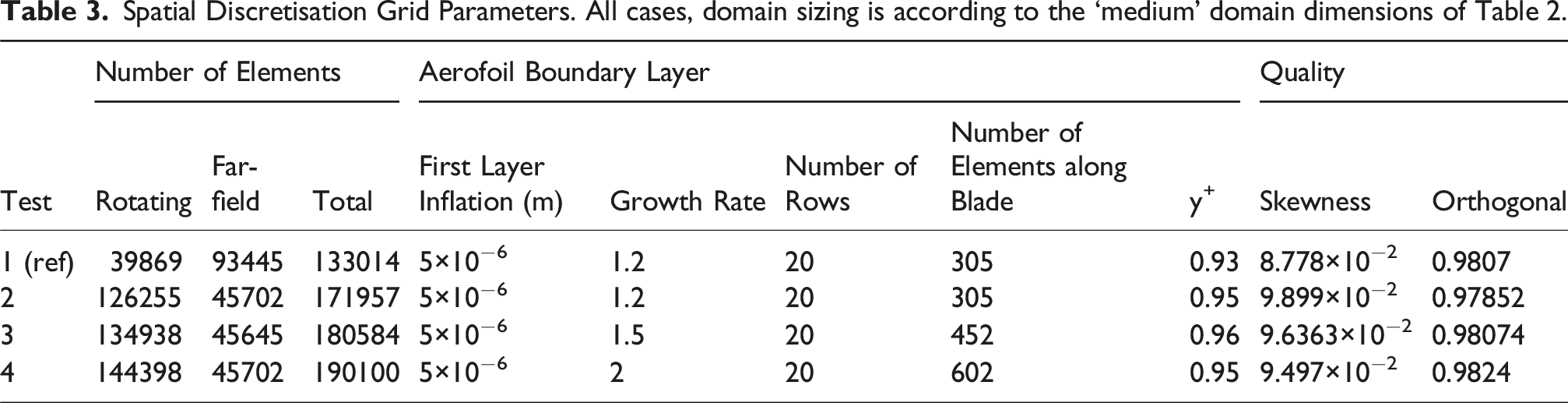
Spatial Discretisation Grid Parameters. All cases, domain sizing is according to the ‘medium’ domain dimensions of Table 2.

Test	Number of Elements			Aerofoil Boundary Layer					Quality
Test	Rotating	Far-field	Total	First Layer Inflation (m)	Growth Rate	Number of Rows	Number of Elements along Blade	y⁺	Skewness	Orthogonal
1 (ref)	39869	93445	133014	5×10⁻⁶	1.2	20	305	0.93	8.778×10⁻²	0.9807
2	126255	45702	171957	5×10⁻⁶	1.2	20	305	0.95	9.899×10⁻²	0.97852
3	134938	45645	180584	5×10⁻⁶	1.5	20	452	0.96	9.6363×10⁻²	0.98074
4	144398	45702	190100	5×10⁻⁶	2	20	602	0.95	9.497×10⁻²	0.9824

Figure 4.

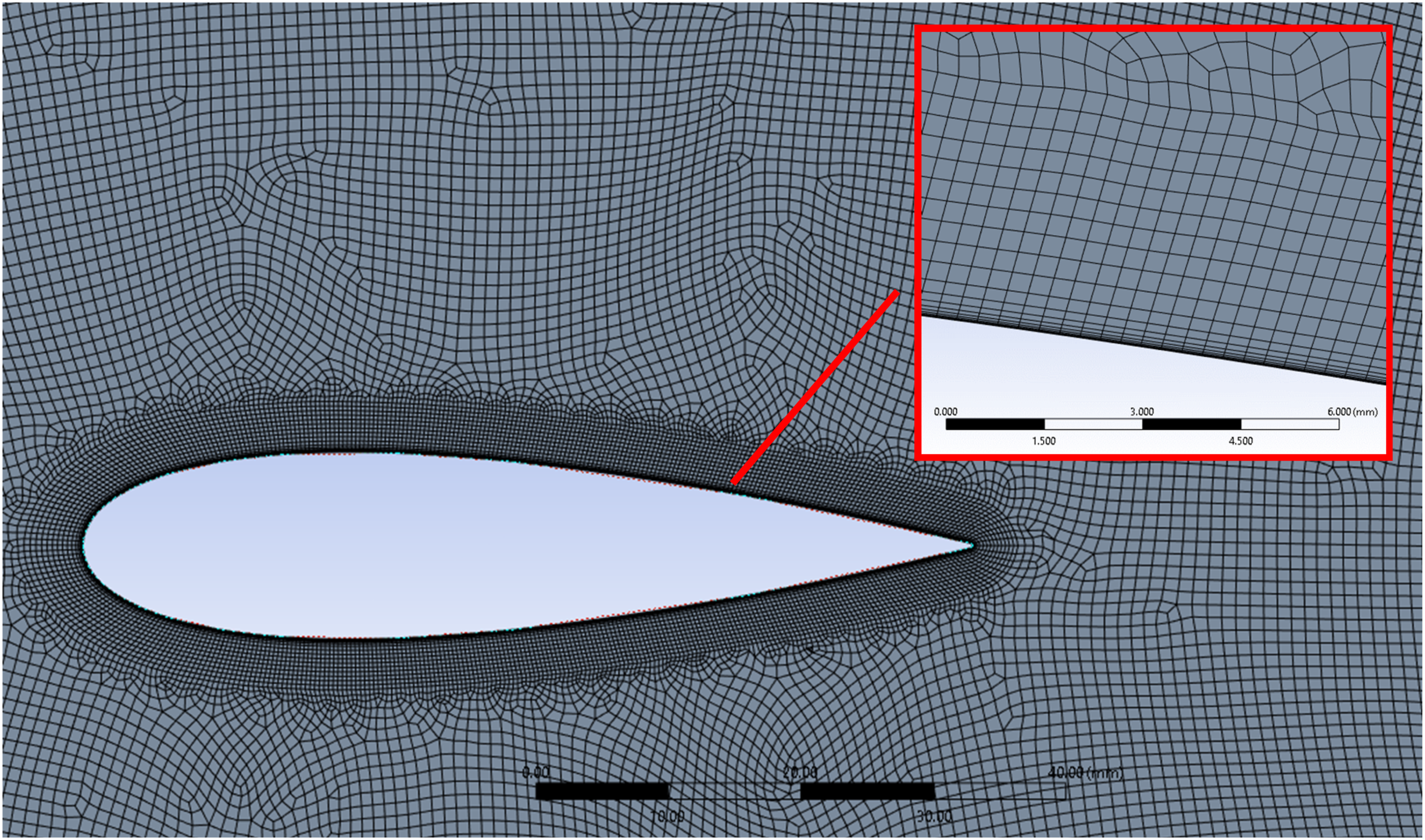
NACA0021 First layer of thickness and elements along the aerofoil.

For each mesh of Table 3 a test simulation was conducted at λ = 2.5. To expedite the time in developing the wake for three of the test cases, the reference mesh was run first, for 40 revolutions, and the flow field result obtained then used as the initial flow state of the other test cases in Table 3. Each of cases 2, 3 and 4 were subsequently run for two rotor revolutions, with the force data for the rotor collected throughout the second revolution. For these λ = 2.5 cases, the time step of 8.49 x 10⁻⁵s (correspond to 0.02° step) ensured a maximum value in the domain of $C F L \approx 1$ .

The coefficient of torque, C_T, for each of the test cases of Table 3 is shown in Figure 5. It is evident on the initial mesh refinement from 5 mm to 1 mm in the aerofoil BOI, the torque increases at various stages of the rotational cycle of the rotor, most notably at azimuth angles of approximately 100, 205 and 340°. At these locations the torque seems to shift to the right which may be attributed to the delay of flow separation from the aerofoil due to the increased resolution in the blade region. The addition of elements along the aerofoil further shifts the torque which again can be recognised as the additional elements refining the separation point along the aerofoil. Due to the large quantity of simulations required for the study, mesh 3 (refer to Table 3) was selected which was a suitable balance in computational time and error.

Figure 5.

For each of the meshes for 3-blades rotor at λ = 2.5. The Single-Blade coefficient of torque shows a difference in the grids at approximately azimuth angle of 100°, which supports the total torque.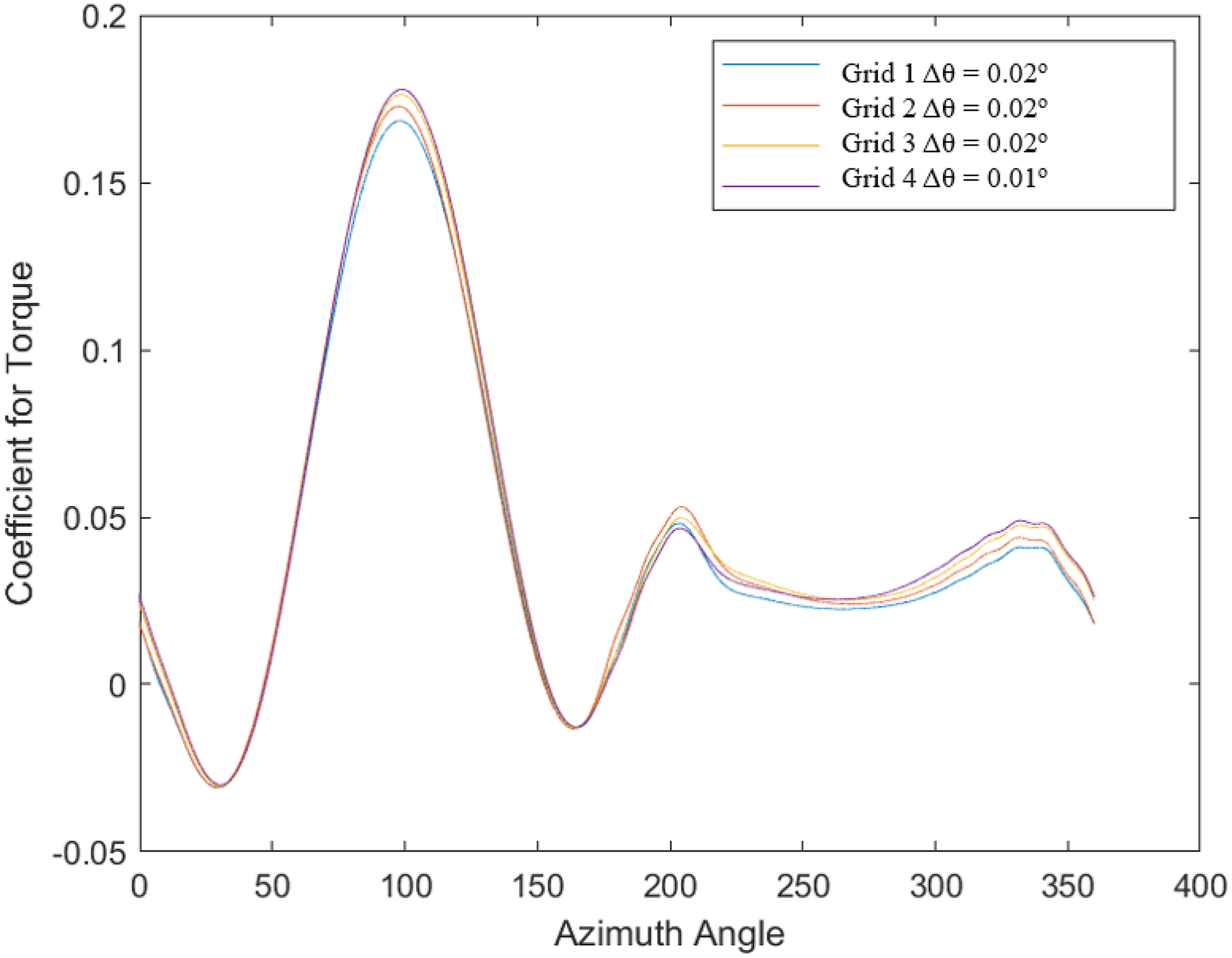

The time-step set-up

The unsteady simulation time step is determined considering the mesh size at the interface between the rotating and inner mesh zones (interface condition), Courant-Friedrichs-Lewy (CFL) number and the total time required to reach quasi steady-state flow.

The rotating BOI was set as mesh motion with a rotation speed expressed as $ω = \frac{λ U_{\infty}}{R} (\frac{r a d s}{s})$ . This enabled the rotating domain to advance at a predetermined rotational speed in radians per second as a function of λ governed by incoming fluid stream velocity and the radius of the turbine. This expression enabled λ to be varied within Fluent^®.

The distance that any data fluid particles within the mesh during a time step can be described using the Courant-Friedrichs-Lewy (CFL) number $C F L = \frac{U Δ t}{Δ x}$ , where U is the local magnitude of velocity of the flow, and $Δ x$ is the local characteristic size of the mesh cells (assumed in the direction parallel to the local flow velocity). To obtain accurate results it was desired that the value of this criterion at any location in the domain never exceeded $C F L \approx 1$ , such that each cell receives the data from the adjacent cell and no cell is missed. This is particularly important around the aerofoil. This region had both the smallest characteristic size of the overall mesh (length ∼ 3 × 10⁻⁴ m, thickness ∼ 5 × 10⁻⁶ m), and the highest magnitude of velocity (∼3.3 m/s) and was therefore the critical zone for satisfying $C F L$ . Accordingly, the time step size required to meet $C F L \approx 1$ for this region should be lower than 10 × 10⁻⁵ s; as a consequence of this time step size and the combination of larger cells and lower velocities elsewhere, all other zones of the domain had $C F L < 1$ . The representative $C F L$ contour around a blade shown in Figure 6 is indicative of adequately small time step with regard to the $C F L$ criterion.

Figure 6.

Top Aerofoil Mesh Grid. The region around the aerofoil has a 1<CFL <2 where the data from the adjacent cells may be missed across the individual elements.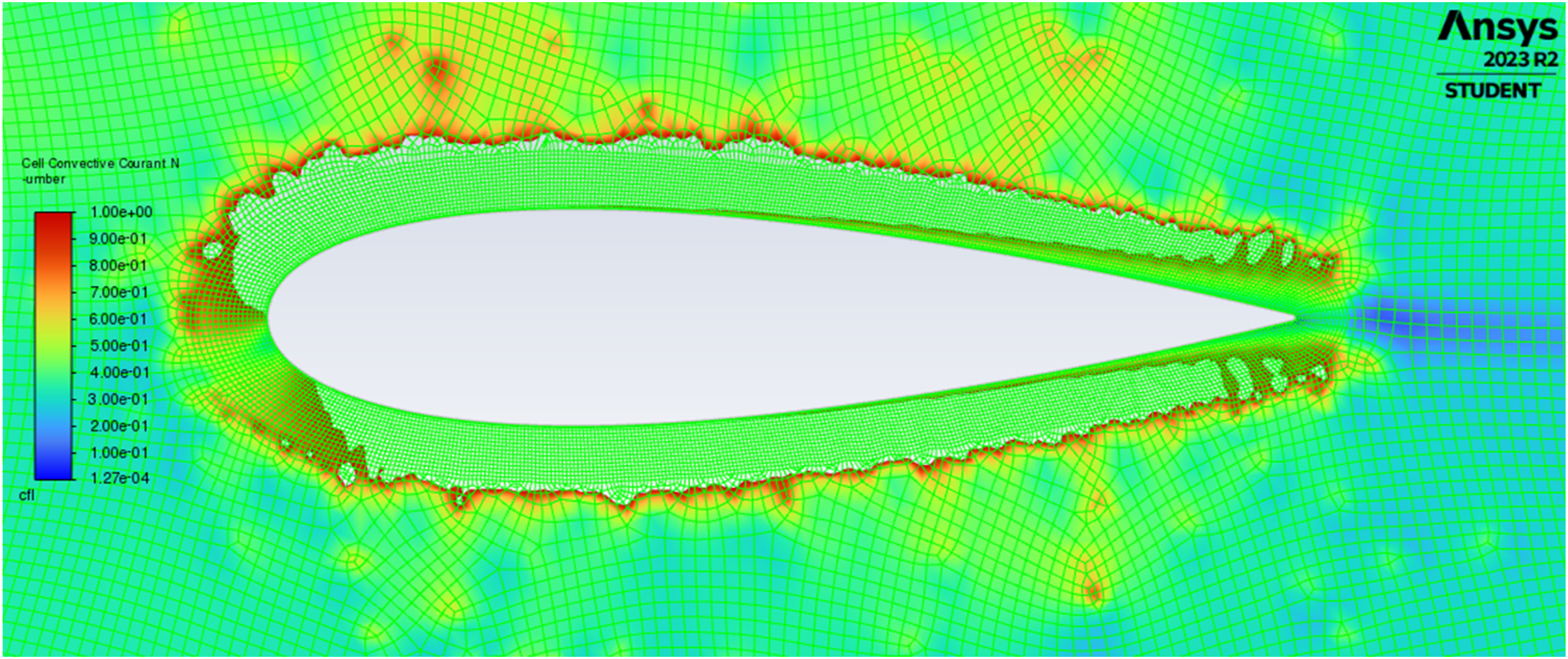

Another important region is the interface of the far field domain and the rotating domain. Each cell at the interface of the rotating domain must also receive the data from the far field domain such that at each time step the rotating domain only moves an angular distance which enables the data from the far field domain to transfer to each cell of the rotating domain and vice versa. The angular distance travelled by the rotating BOI during each time step is expressed as,

Δ θ = ω (\frac{180}{π}) Δ t

(3)

To ensure the afore mentioned interface condition is met, $ω (\frac{180}{π}) Δ t / Δ θ_{int} < 1$ , time step, $Δ t$ is set such that,

Δ t < Δ θ_{int} / [ω (\frac{180}{π})]

(4)

where

Δ θ_{int}

is the angular spacing of the interface cells (the largest of either the inner or rotating domain) with reference to the centre of the rotating zone.

To ensure that the analysed result is that of quasi steady state, the total time independence must be carefully determined. This was determined by assessing the flow time required after flow condition change. For example, when λ was adjusted, the change in λ has an instantaneous effect on the turbine; however, the flow field around the aerofoil and throughout the rotor zone more generally – including the rotor wake – takes a period of time to develop to a new quasi-steady state corresponding to the new value of λ. It was determined that the solutions were suitably converged post-λ-adjustment after four subsequent revolutions of the rotor.

Result and discussion

Comparison of coefficient of performance, C_p

The coefficient of performance, C_p, curve is commonly used as the indicator of the performance characteristic of a turbine, including C_p,max and λ_opt. Additionally, the ability to self-start may be assessed by the degree to which this curve plateau or dips, that is, whether torque dip is present. For HDT, the C_p values are obtained on the basis of cycle-averaged torque as C_p = C_t λ, and positive C_p accords to positive averaged torque, and hence, turbine acceleration after the cycle. Figure 7 displays the C_p - λ curves of the different c/r turbines, namely, 0.268 and 0.804. The corresponding maximum coefficient of powers, C_p,max are 0.38 and 0.3, while optimal tip-speed ratios λ_opt are 1.75, and 2.1, respectively, for c/r = 0.804 and 0.268. The turbine with the longer blade (c/r = 0.804) displays greater C_p across all tip-speed-ratios. To assess turbine starting ability, the trend of C_p in the range λ < 1 (shaded range in Figure 7) is used as an indicator. In this λ range, the C_p curve of the shorter blade turbine (c/r = 0.268) exhibits, within the λ range 0 < λ < 0.5, low steady C_p and marginal increase thereafter on to λ = 1 – an indication of low torque during the start-up phase. This contrasts to the higher C_p trend of the longer blade turbine (c/r = 0.804), which at λ = 1 reached a C_p value (C_p ∼ 0.15), five times larger than that at the same λ of the shorter blade case (C_p ∼ 0.03). This indicates greater torque produced by increasing c/r, with the higher torque of c/r = 0.804 compared to c/r = 0.268 persisting until the free-spin λ of approximately 3.5. It is also notable for the higher c/r turbine that the peak in C_p occurred at lower λ.

Figure 7.

Coefficient of Performance plot of the single-blade and three-blade HDT. The shaded region is critical transient starting phase. Coloured curves are visible on the online version.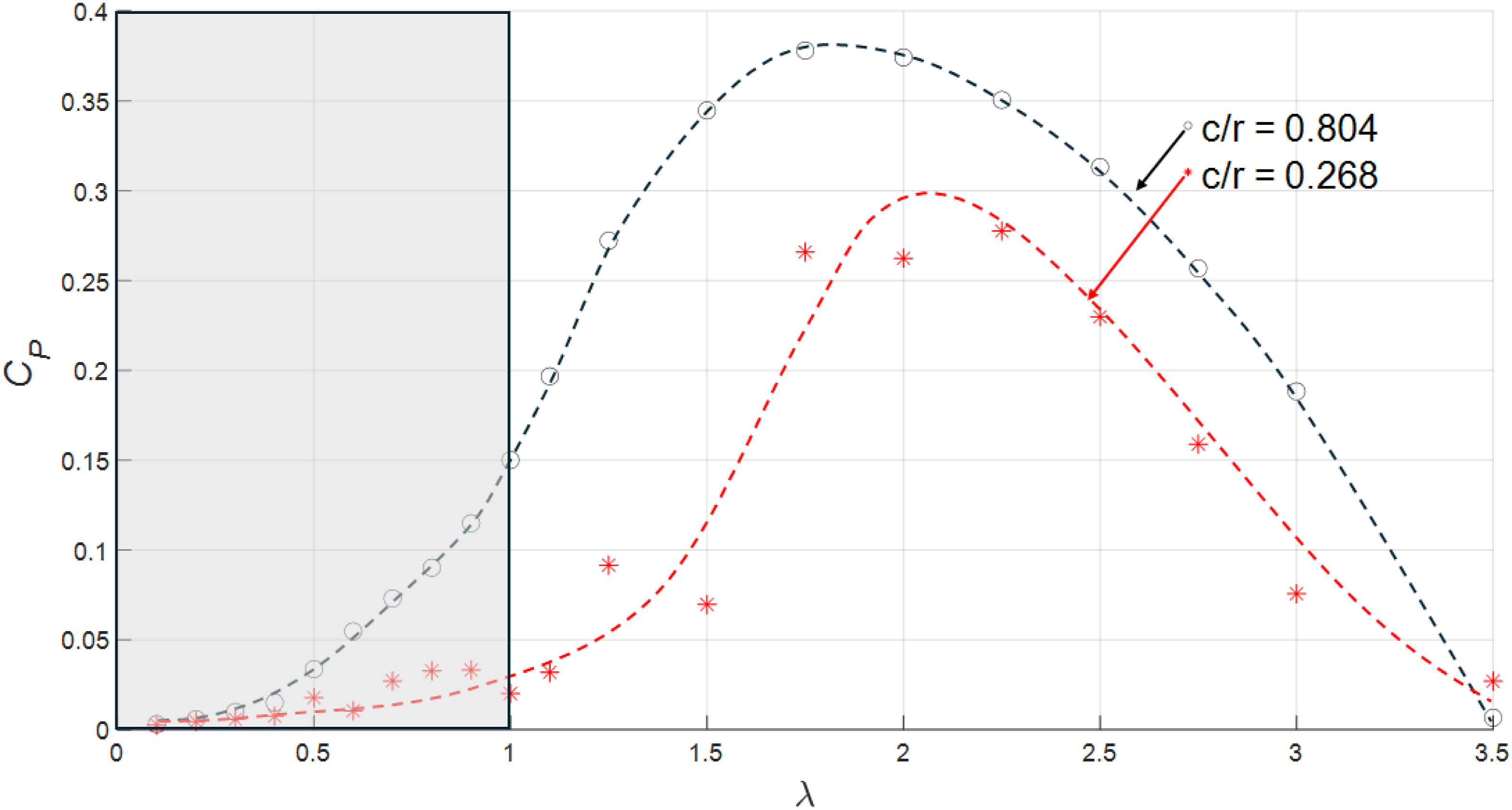

The increased torque performance of the single-blade HDT at lower λ could be related to several factors. The single-blade configuration with the increased chord length has a higher chord Reynolds Number. The increase in aerofoil chord length also results in thicker aerofoil (Lissaman 1983). The increased chord Reynolds number subsequently affects the boundary layer on the aerofoil such that the boundary layer tends to remain attached for longer, resisting separation. This delayed separation helps to maintain the smooth flow of fluid over the aerofoil, preventing the formation of leading-edge vortex (LEV) and flow separation thus reducing the likelihood of stall.

To probe the source of the observed greater torque of the longer blade, the torque variation with azimuth angle, θ and the flow field around the blade at λ = 0.5 and 0.9 are analysed in detail in the next section.

Comparison of torque variation per revolution and the flow field correlation

The blade chord length to rotor radius ratio, c/r, influences the flow curvature coming from the aerofoil on its circular path (Balduzzi et al., 2014). Symmetrical blades with large c/r essentially behave like virtually cambered aerofoil in a rectilinear flow. Virtual camber result in increases of lift coupled with a delay in stall (Migliore et al., 1980), potentially improving the torque generation. To understand at which instance torque is enhanced, variation of torque with azimuth angle position, $θ$ is analysed, refer to Figures 8 and 10 for λ = 0.5 and 0.9, respectively.

Figure 8.

Variation of Coefficient of Torque with azimuth angle of the single-blade and three-blade HDT for λ = 0.5. The black dots show instances θ = 30°, 60^o, and 90°, of flow fields shown in Figure 10. Coloured curves are visible on the online version.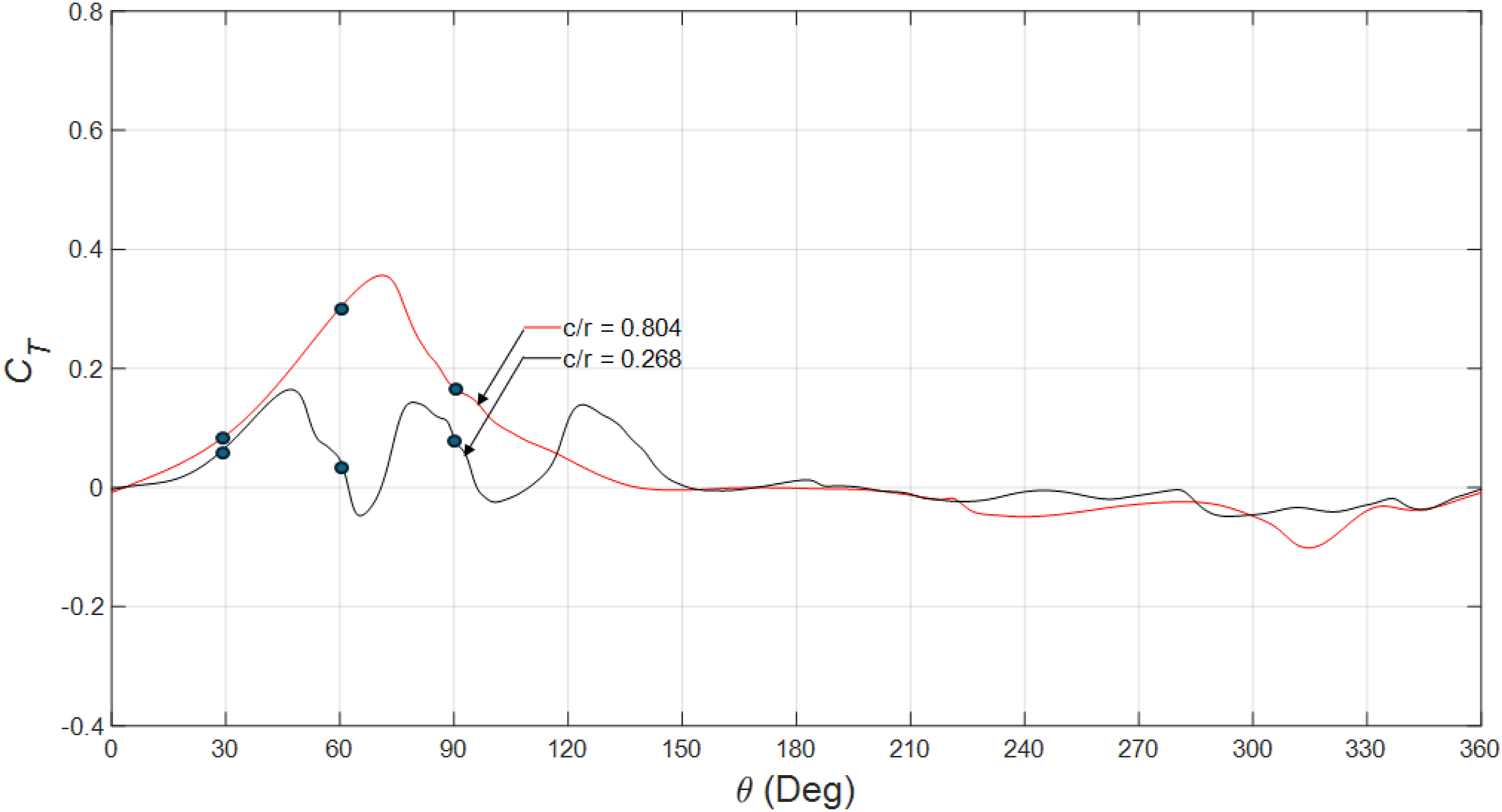

Consider first λ = 0.5, the torque variation with θ (Figure 8) shows significant difference in terms of magnitude and fluctuations of the torque during the upwind passage of the blades between c/r = 0.268 and 0.804. This is especially so whilst θ = 45° – 120° where lift is the positive contributor to torque (see also Figure 10). Up to θ = 30° torques are similar with the c/r = 0.804 torque slightly greater.

To understand the physics, flow fields around the blade at θ = 30°, 60° and 90° for λ = 0.5 are analysed in Figure 9. Torque is generated mainly in the turbine upwind half. Turbine with larger c/r (=0.804) clearly shows higher torque than the lower c/r (=0.268) for most part of the upwind half (Figure 8). The sustained positive torque is associated to attached and shear layer growth (Le Fouest et al., 2023). The higher c/r blade maintains attached shear layer sustained for longer (Figure 9, right column). Up till θ = 30°, the flow fields of both cases are similar (top rows of Figure 9). When θ = 60°, α = 40.9°, the flow around the blade of the c/r = 0.804 case is still attached with no sign of leading-edge vortex generation, in contrast to c/r = 0.268 where leading- and trailing-edge vortices have clearly been formed (second row Figure 9). For c/r = 0.804, at θ = 90°, α = 63.4°, leading-edge vortex is formed; however, it appears reattached to the surface instead of detaching. This is in contrast with lower c/r turbine (=0.268), where the leading-edge vortex detaches as shown at θ = 60°, α = 40.9°. The leading-edge vortex detachment and interaction with the trailing-edge are thought as the principal events associated with the upwind torque fluctuations of the lower c/r case (0.268).

Figure 9.

Vorticity field, ω_z, of the three-blade (left) and the single-blade (right) for λ = 0.5. HDT at θ = 30° (top), 60° (middle), and 90° (bottom). The corresponding incidence angles are α = 20.1°, 40.9°, 63.4° for θ = 30^o, 60^o, 90^o, respectively. Coloured curves are visible on the online version.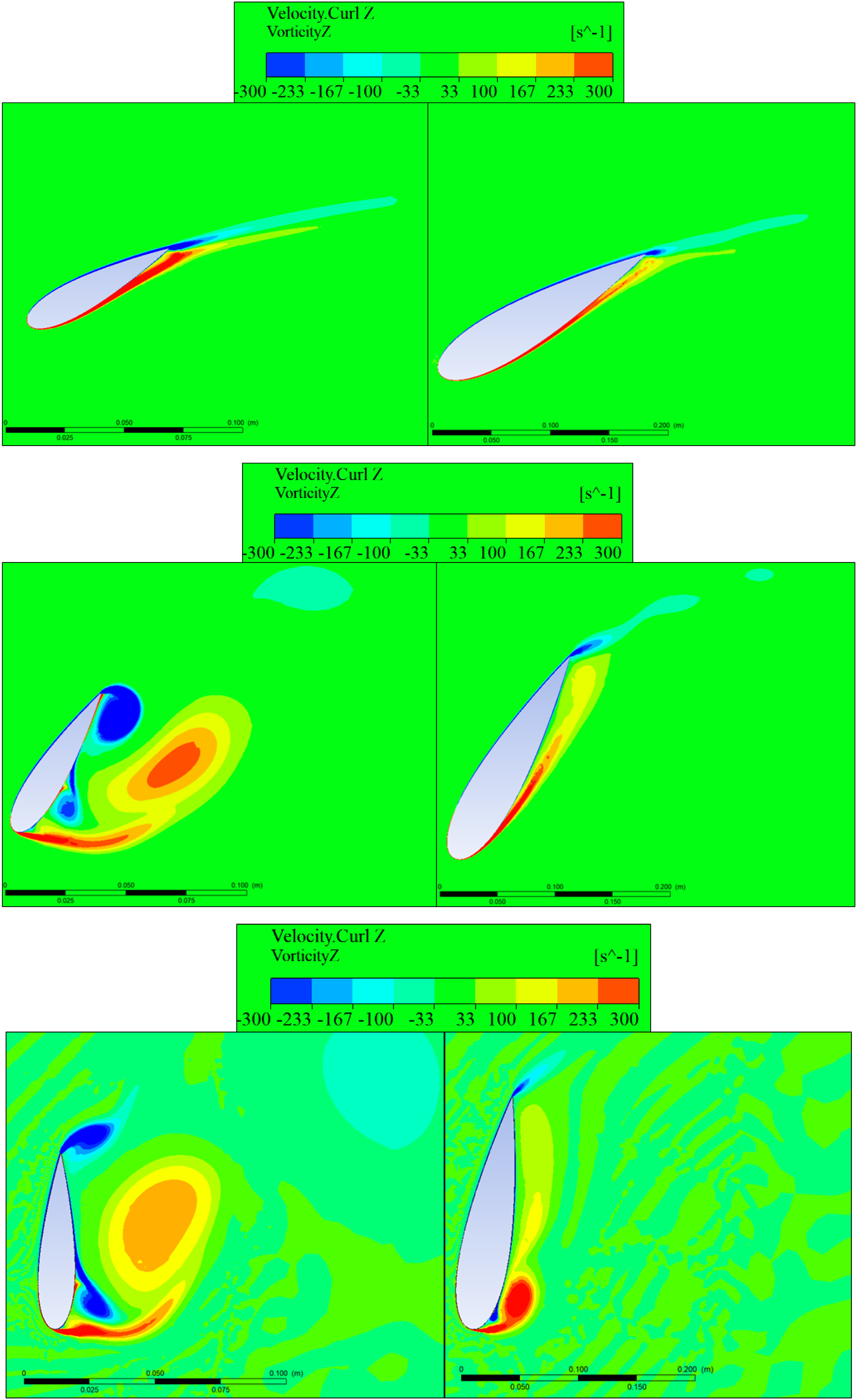

Considering the trailing-edge, the trailing-edge vortex (TEV) seems suppressed with c/r = 0.804. This explains why the leading-edge vortex can approach the surface and reattach. There is clear suppression of both trailing- and leading-edge vortex generation, resulting in attached flow throughout the majority of the upwind portion of the blade transit. The contrast in the flow field between c/r = 0.268 and 0.804 suggests there is a dynamic event. This is most likely related to virtual morphing (Keisar et al. 2020, 2024).

Consider now λ = 0.9, the torque variation with θ (Figure 10) as with λ = 0.5, also shows significant difference between c/r = 0.268 and 0.804 during the upwind passage of the blades. Up to θ = 60°, only slightly greater torque with c/r = 0.804 than 0.268. Between θ = 60° and 150° torque of c/r = 0.804 are clearly greater than 0.268. As α = 90° occurs at θ = 154°, lift contribution is the positive contributor in the most of upwind zone, that is, θ up to 154°.

Figure 10.

Variation of Coefficient of Torque with azimuth angle of the single-blade and three-blade HDT for λ = 0.9. The black dots show instances θ = 60^o, 100^o, and 150^o, of flow fields shown in Figure 11. Coloured curves are visible on the online version.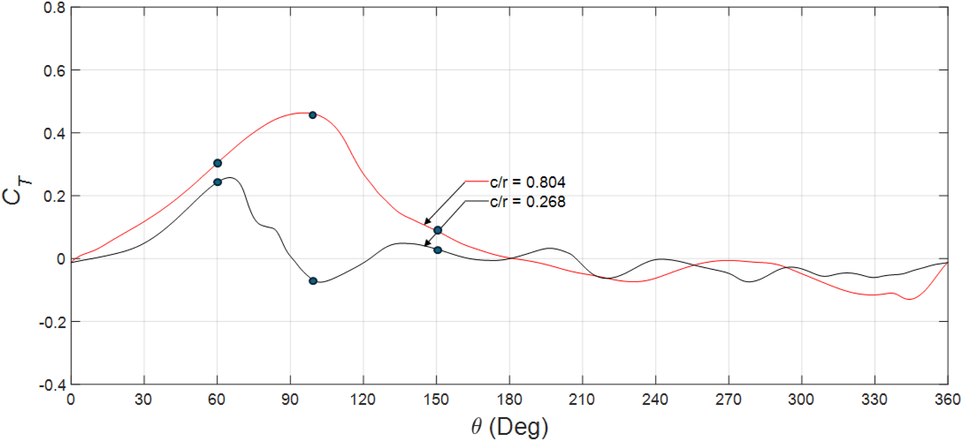

To explain, flow field at θ = 60°, 100° and 150° are analysed (Figure 11). The corresponding α at these instances are 31.7°, 53.6 and 86.1°. Up to θ = 60° the flows remain attached for both turbines. This explains torques from both turbines are also relatively similar. At θ = 100° the flow fields are quite different. The flow field around the shorter blade (second row left of Figure 11) shows significant leading vortex shedding, flow separation on the suction side, with formation of strong trailing-edge vortex. The trailing-edge vortex contributes to the detachment of the leading-edge vortex. On the contrary, flow remains attached and much smaller trailing-edge vortex is formed for the longer blade (second row right of Figure 11). The difference of the flow fields correlates with the difference in lift and hence torque generated on the blade.

Figure 11.

Vorticity field, ω_z, of the three-blade (left) and the single-blade (right) for λ = 0.9. HDT at θ = 60° (top), 100° (middle), and 150° (bottom). The corresponding incidence angles are α = 31.7°, 53.6 °, 86.1° for θ = 60^o, 100^o, 150^o, respectively. Coloured curves are visible on the online version.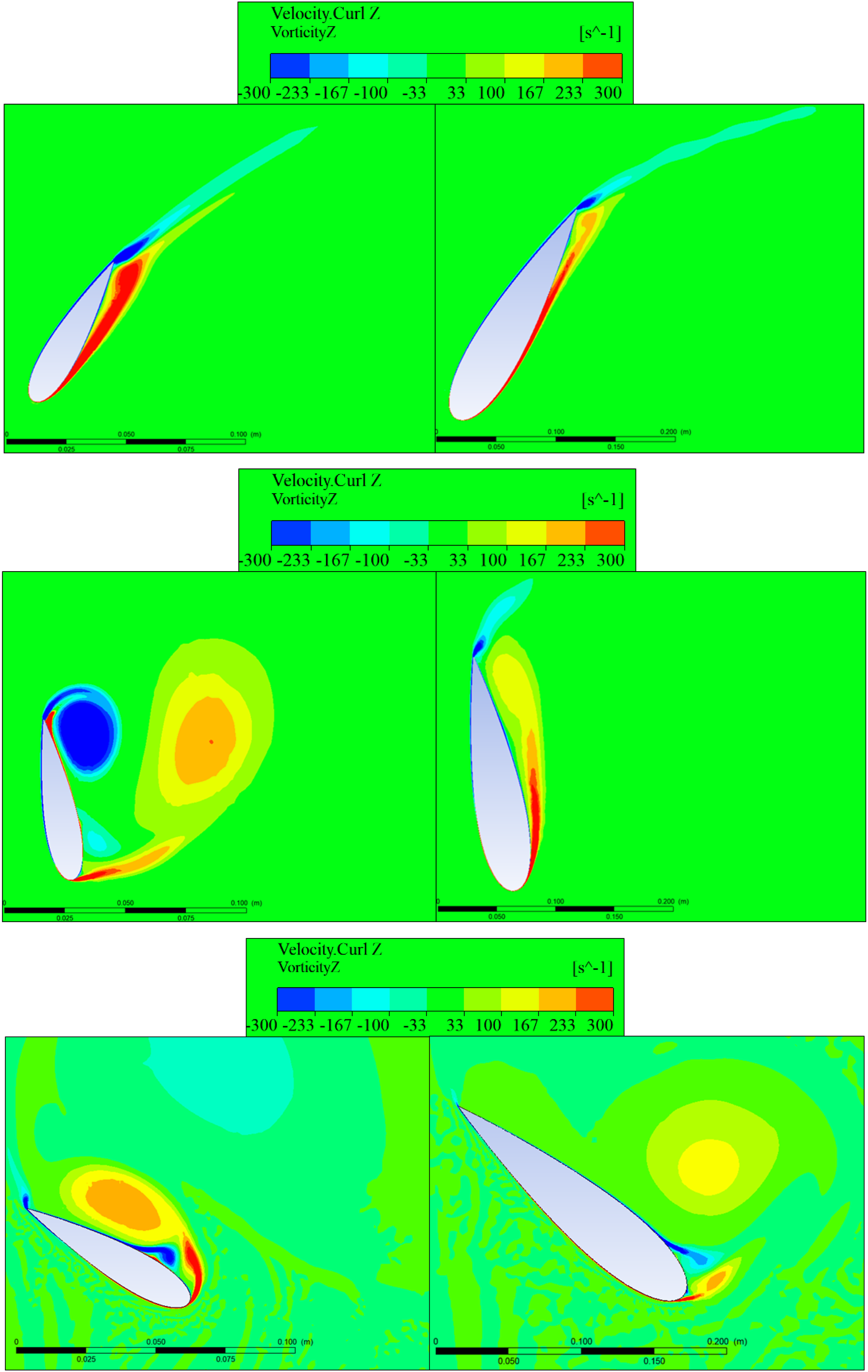

The preceding analysis shows that although subject to the same α, the flow fields around the blade are significantly different. The explanation is thought to be related to the complex curvilinear flow around the blade, manifested due to continuously varying virtual cambering ‘virtual morphing’. The effects of which are amplified by increases in instantaneous blade pitch rate. The influence of the pitch rate on the extent of virtual cambering of the blades in the two c/r cases is analysed in the following section.

Variable pitched rate and virtual morphing–based explanation

In previous section, it is clearly seen that the flow fields around the blades of the two cases of c/r = 0.268 and 0.804 are different. This section presents analysis of the possible mechanism with the intent of explaining the differences. During the transient starting phase, when λ is still <1, the incidence angle, α_p varies from 0° to 360° as given by equation (5). Note that α_p is the incidence angle at the connection point.

α_{p} = \tan^{- 1} (\frac{\sin θ}{λ + \cos θ})

(5)

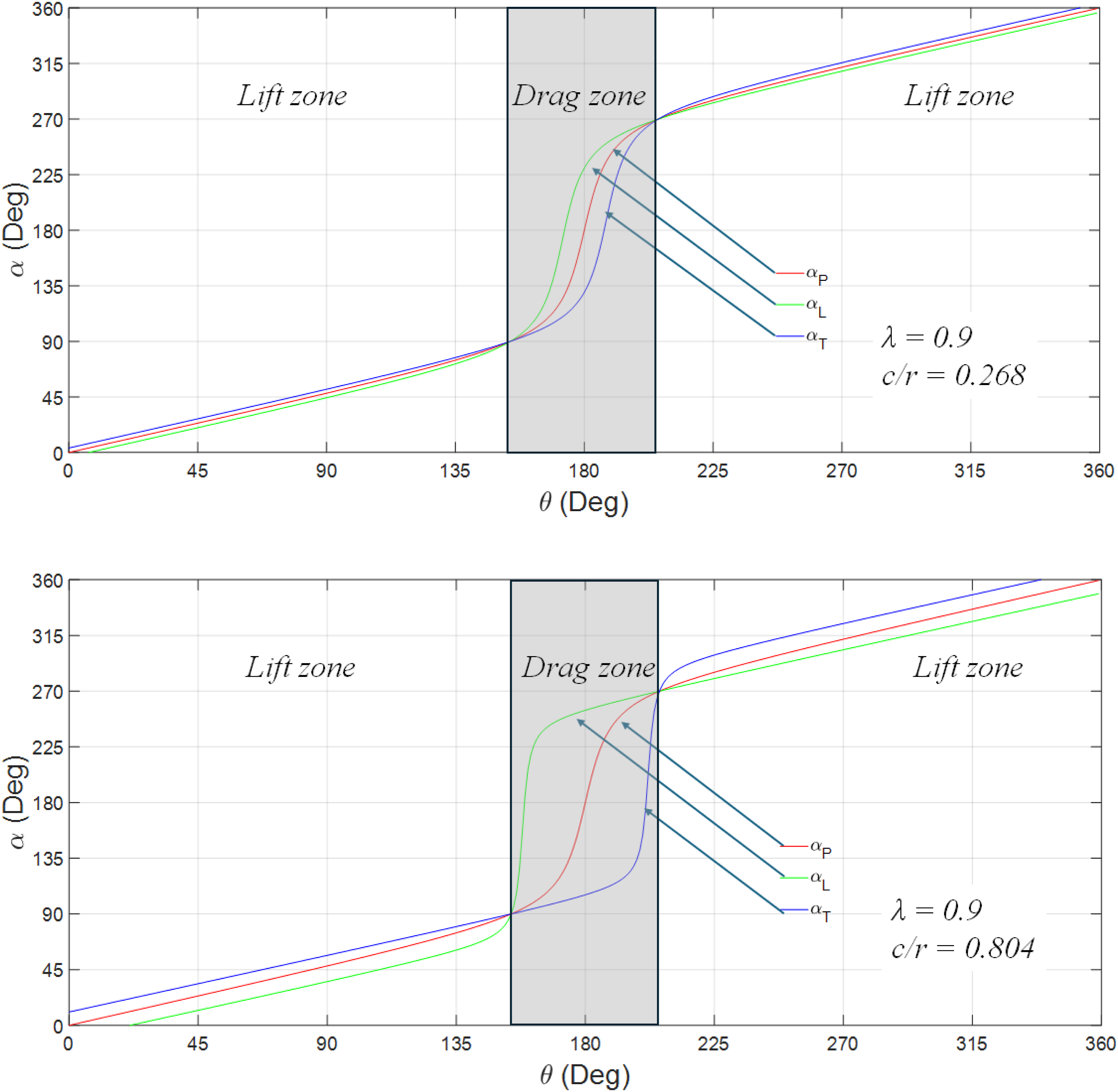
Blades with incidence angle, α_p, varies from 0° to 360° is analogous to rotating isolated aerofoil in freestream. For λ < 1, the lift force and drag force intermittently make positive contribution to the torque. Lift is favourable when incidence angle is less than 90° or greater than 270° (Figure 12). For example, as shown in Figure 12, drag is favourable between at 120° < θ < 240° for λ = 0.5, and between 154° < θ < 206° for λ = 0.9. Overall, the trend for the λ < 1 regime is θ range within which drag is favourable reduces as λ increases from zero (0) through to 1. Outside these ranges only lift positively contributes to torque. Considering torque is generated predominantly in the upwind zone, when the torque is low in this zone, the turbine is prone to the occurrence of torque plateau (or torque dip). In the λ < 1 regime, because lift and drag forces on a given blade positively contribute to torque in a sequential manner as the blade repeatedly transits around its circular path about the turbine centre, during the azimuth regions within which lift accords to positive torque the lift-to-drag ratio ideally would be large to ensure stall does not occur, and small (lift-to-drag ratio) during the azimuth regions in which drag is the positive contributor to torque.

Figure 12.

For λ < 1, blades incidence angles vary from 0° to 360° (revolving aerofoil). For α < 90° or >270°, lift contributes to positive thrust whilst 90° < α < 270° drag contribute to positive thrust. Note also approximately constant rate of change of α in the lift zone. α in this figure represents α_p i.e. the apparent incidence at the mounting point (see Figure 14). Coloured curves are visible on the online version.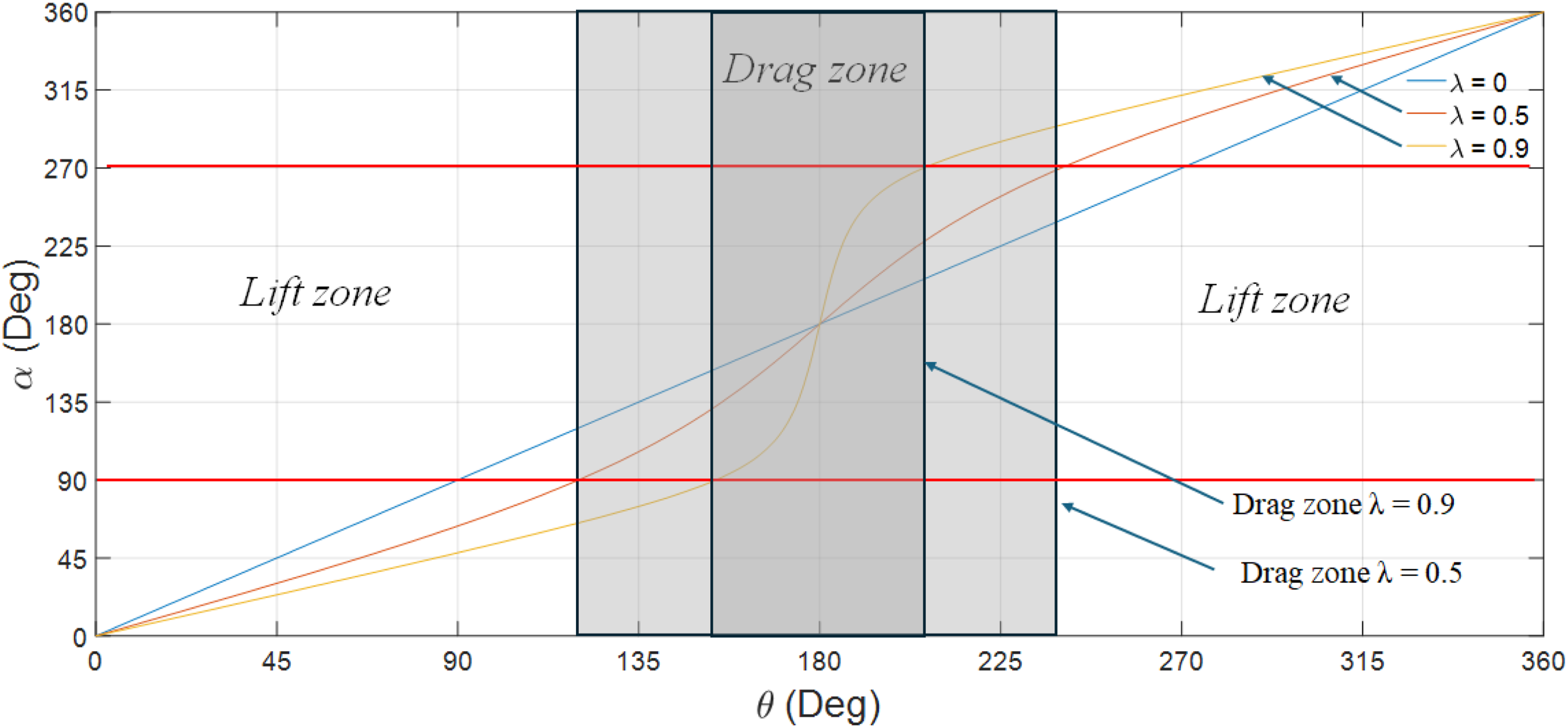

Due to the curvature, the effective incidence angle at the connection point, α_p of turbine blades is constantly changing from 0° to 360° within a cycle. Additionally, the chord-local incidence angle, defined as the angle between local relative velocity and the chord line, varies as illustrated in Figure 13. This is local incidence angle varies with position on the chord, for example, leading-edge (L), connection point (P) and trailing-edge (T) such that α_L < α_P < α_T as shown in Figure 13. As blade orbits, α_L, α_P and α_T constantly vary resulting in virtually morphing blade.

Figure 13.

Variation of incidence angle, α, along the chord line. The tangential velocity varies with curvature radius. As this radius varies, the local tangential velocity also varies along the chord. Additionally the angle of the local tangential velocity to the chord line also varies. This results in variation of local incidence angle with position along the chord line. It is shown that α_L < α_P < α_T.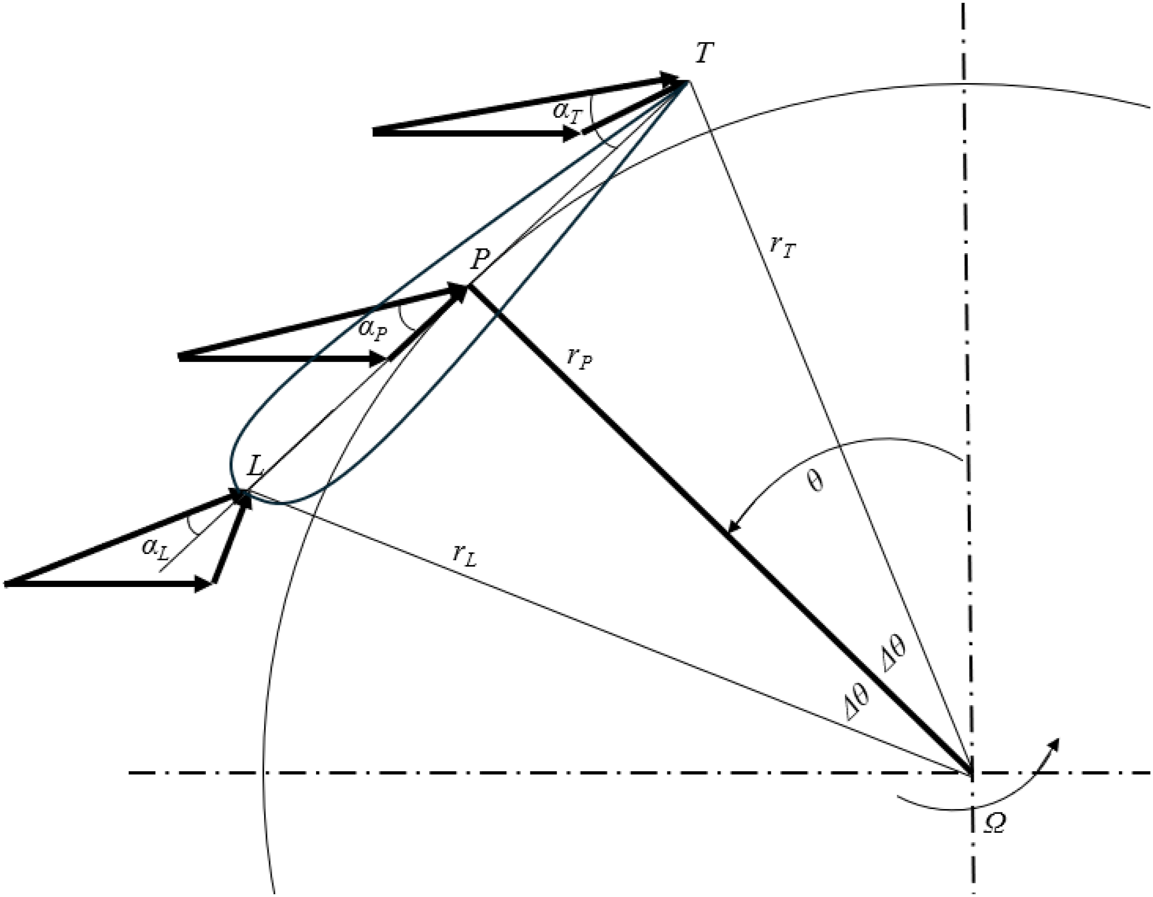

Local incidence angle, $α$ along chord line axis, x is given by (Keisar et al., 2024)

α (x) = \tan^{- 1} (\frac{\sin (θ + β)}{λ^{'} + \cos (θ + β)}) - β

(6)

With

β = \tan^{- 1} (\frac{x_{p} - x}{c} ε)

(7)

λ^{'} = \frac{λ}{\cos β}

(8)

where

ε

is c/r; and

x_{p} = \frac{c}{2}

is mid-chord strut-blade connection point. The leading-edge and the trailing-edge coordinates are x = 0 and x = c, respectively.

The variation of the local incidence angle with azimuthal angle, θ is illustrated in Figures 14 and 15 for λ = 0.5 and λ = 0.9, respectively, and each for the two c/r cases. The variation is to an extent analogous to an aerofoil with flaps and slats as often used on aircraft, incorporated to obtain increased lift performance during take-off and landing phases of flight. Considering HDT, during the lift zone, α_L < α_P < α_T is analogous to the slat pitches down and the flap pitches us. This results in the flow remain attach hence maintain lift and increase thrust. During the drag zone, α_T < α_P < α_L, now the slat pitches up and the flap pitches down. The effect on drag is increased thus improves thrust in this zone too. The variation of local incidence angle along the chord becomes more pronounced as λ approaches 1. These effects are clearly amplified with c/r as shown by comparing the variation of the drag zone of Figures 14 and 15.

Figure 14.

Variations of incidence angle of leading-edge, α_L; connection point, α_P; and trailing-edge, α_T for λ = 0.5 and c/r = 0.268 (top figure) and 0.804 (bottom figure). Note the switch of the angles between the lift zone and the drag zone. Coloured curves are visible on the online version.

Figure 15.

Variations of incidence angle of leading-edge, α_L; connection point, α_P; and trailing-edge, α_T for λ = 0.9 and c/r = 0.268 (top figure) and 0.804 (bottom figure). Note the switch of the angles between the lift zone and the drag zone. Coloured curves are visible on the online version.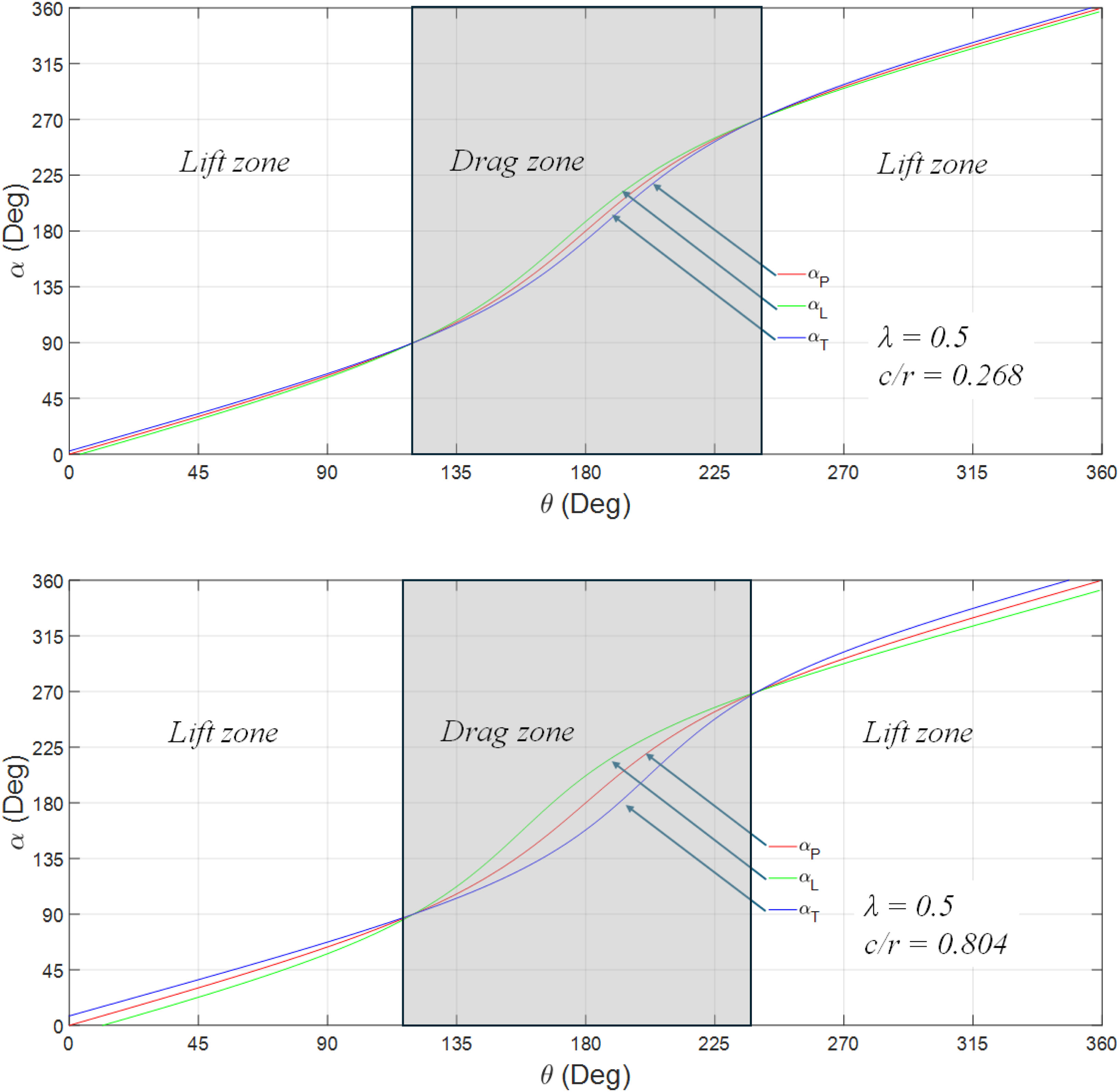

The effect of c/r on virtual camber line changes can be visualised by plotting the virtual camber line variation. The shift of the camber line position, z is related to the chordwise change of the incidence angle given in equation (9) (Keisar et al., 2020).

\frac{d z}{d x} = α_{P} - α

(9)

The virtual camber-line can be obtained by integrating the above equation. The virtual morphed aerofoil results for θ = 90 °, 160°, and 200° for c/r = 0.268 and 0.804; and λ = 0.5 and 0.9 are shown in Figures 16 and 17, respectively. These figures illustrate the continuous virtual morphing of the aerofoil. The degree of the morphing is clearly amplified with c/r and λ.

Figure 16.

Isolated aerofoil analogy of blade with varying incidence angle and camber at different azimuthal angles. For λ = 0.5 and c/r = 0.268, 0.804. Note the flow is from left to right.

Figure 17.

Isolated aerofoil analogy of blade with varying incidence angle and camber at different azimuthal angles. For λ = 0.9 and c/r = 0.268, 0.804. Note the flow is from left to right.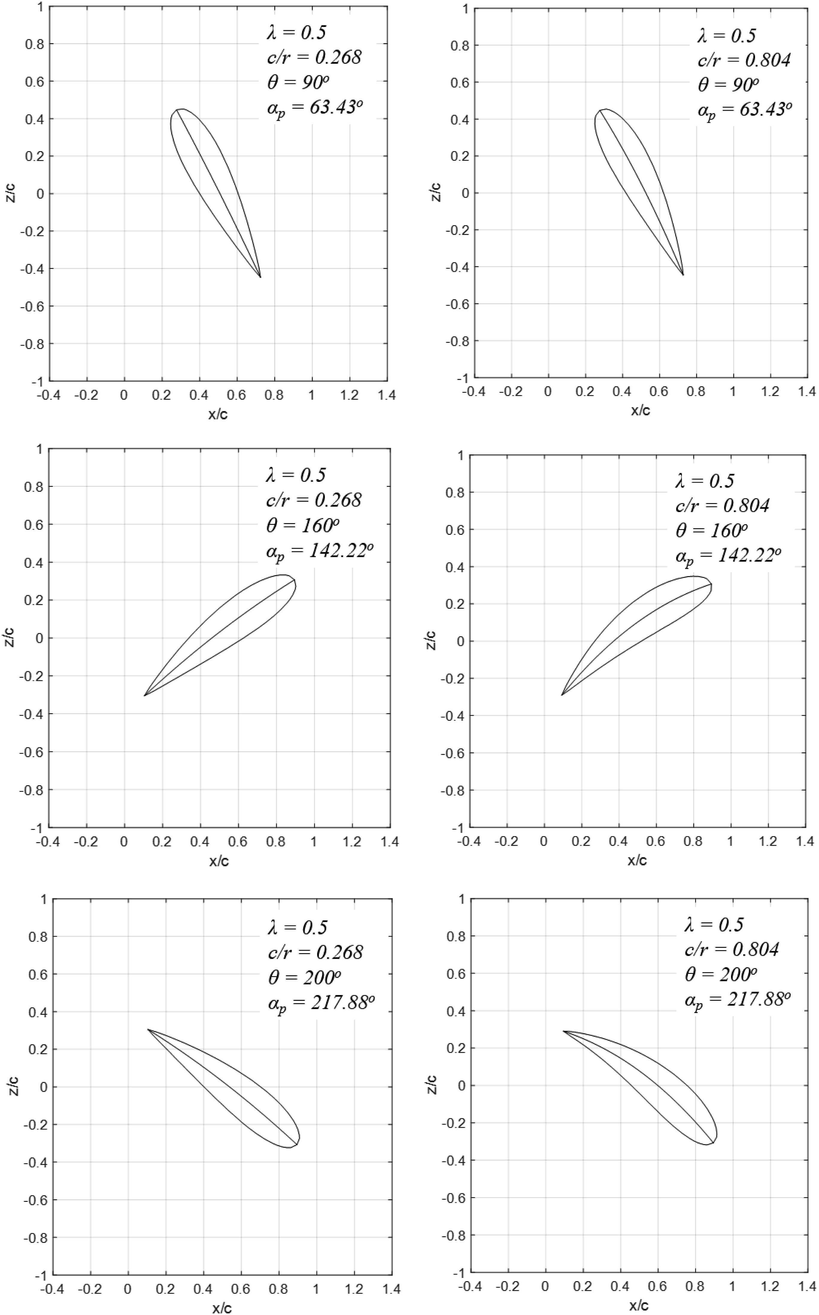

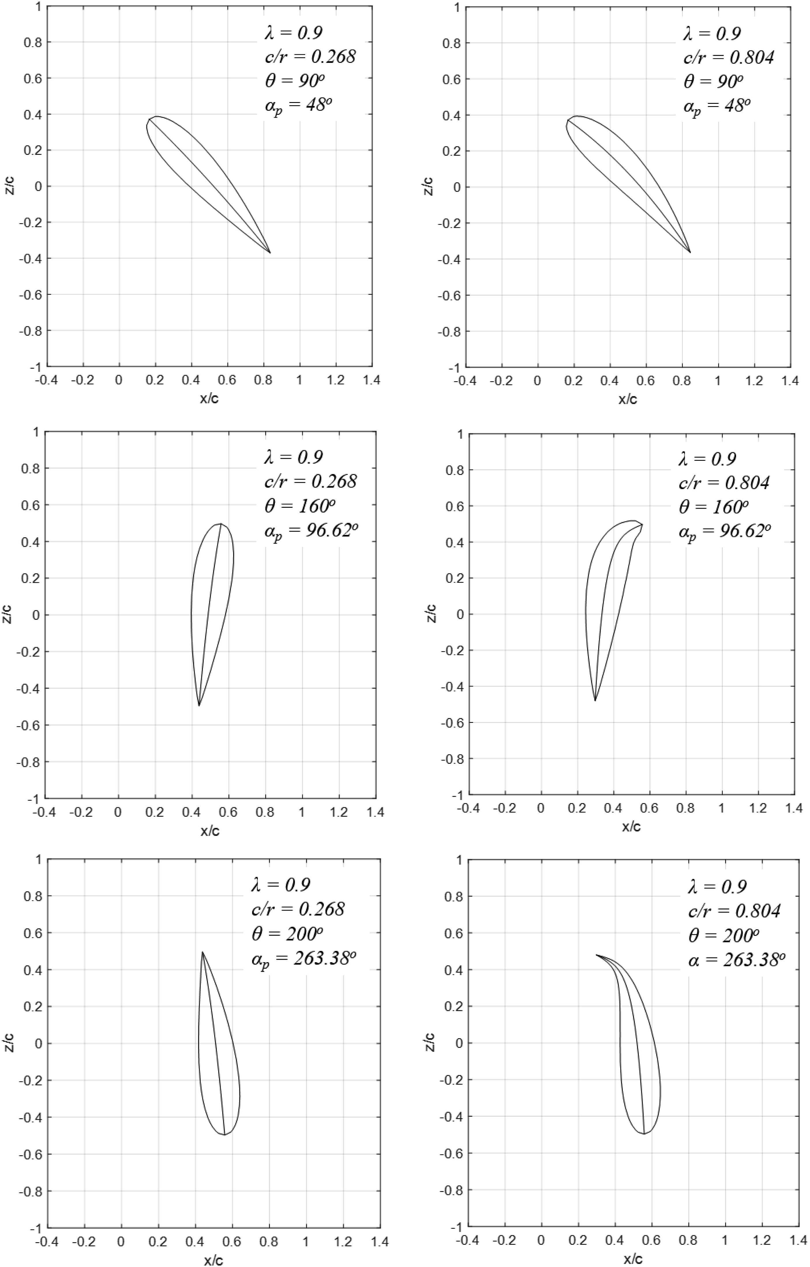
In Figure 16, at λ = 0.5 for θ = 90°, α_P is 63.43°, the virtual nose down leading-edge is more pronounced for the c/r = 0.804. The effect of virtual geometrical morphing is clearly seen in the flow field around the blade (see Figure 9 third row) where the attachment of the leading vortex is apparent. Concurrently, the pitched up trailing-edge results in reduced trailing-edge vortex formation (see Figure 9 third row). The decrease in the incidence of leading-edge is analogous to nose down slat and the increase of trailing-edge incidence angle to pitched up flap. The leading-edge vortex attachment and almost non-existent trailing-edge vortex explain the slightly greater torque (see Figure 8) up to 90° azimuthal position, lift is still favourable. As the blade continues in the orbit, it continues virtual morphing. When θ = 160°, α_P is 142.22° drag is now favourable and the trailing-edge becomes the leading-edge with increased incidence angle. The extended attached flow of the larger c/r (0.804) explains the enhanced torque in the upwind stage of the turbine cycle. Similar effects are amplified as λ approaches 1 (see Figure 17). As λ approaches 1, λ = 0.9 the lift zone is wider hence the benefit of larger c/r affects over wider θ range.

To further assist readers with visualising the extend of the virtual morphing of the turbine blades, Figures 18 and 19 show the morphed aerofoil at different θs and λs, comparing the two different c/r ratios (the short, 0.268 and the long, 0.804 blades). Notice the switch in the curling of the blade from curling in slat pitching down and flap pitching up, from the lift zone to drag zone. Hence lift is enhanced in the lift zone and drag is enhanced in the drag zone in the upwind portion of the turbine cycle. The virtual morphing effect is more pronounced with c/r as shown in the comparison in Figures 18 and 19.

Figure 18.

The morphed aerofoil at different azimuthal angles for λ = 0.5 and c/r = 0.268 (top figure) and 0.804 (bottom figure). The angles shown are the azimuthal angle of the blade, Note the flow is from left to right. Coloured curves are visible on the online version.

Figure 19.

The morphed aerofoil at different azimuthal angles for λ = 0.9 and c/r = 0.268 (top figure) and 0.804 (bottom figure). Note the flow is from left to right. Coloured curves are visible on the online version.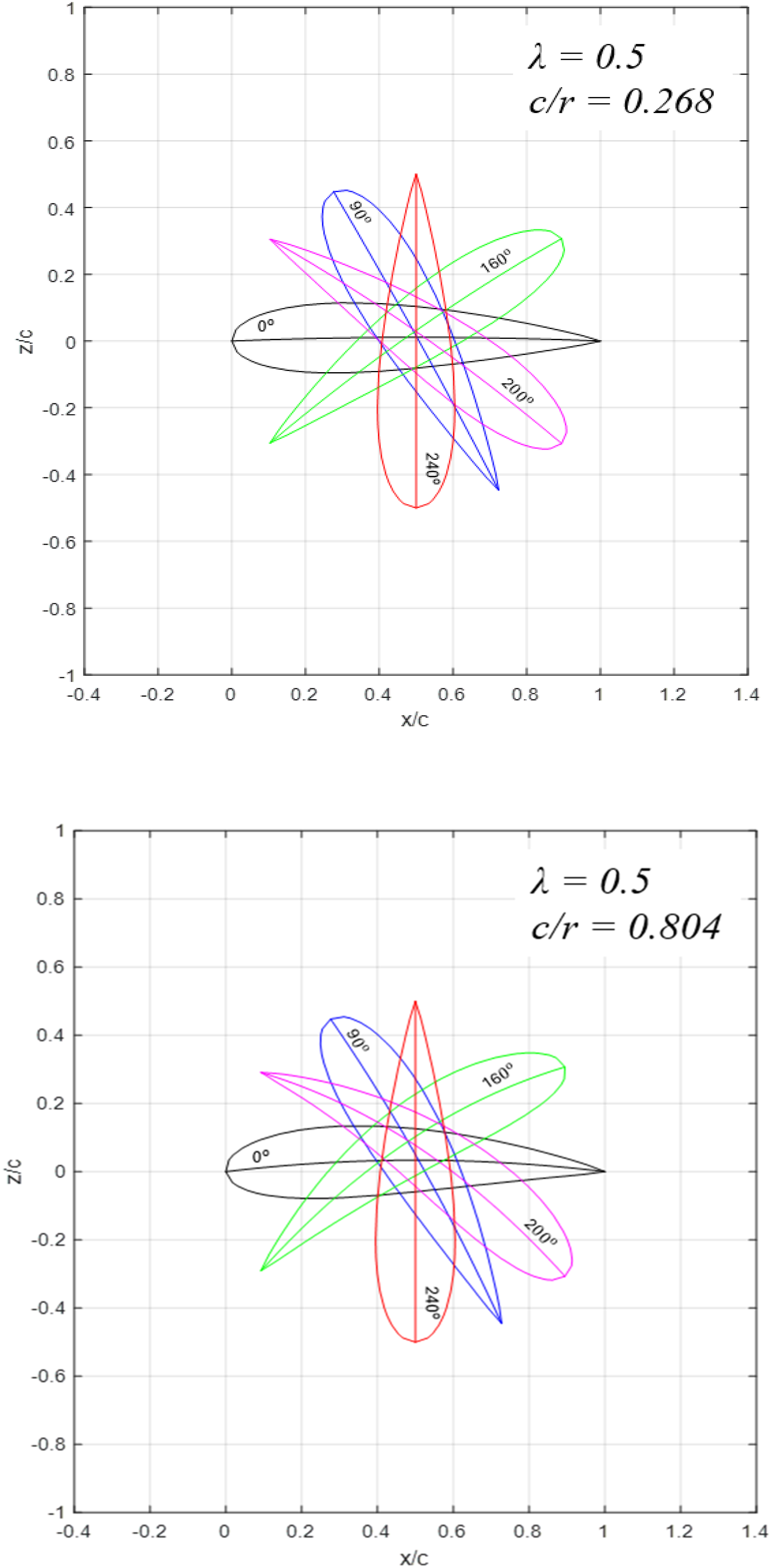

Another effect of varying c/r is the pitch rate. The blade pitch with variable rate or the reduced frequency for HDT is defined as $k = \frac{Ω c}{2 W}$ . As W is the relative incidence fluid velocity, which can be expressed in terms of c and r of the turbine as follows (Worasinchai 2012) the pitch rate equation (10).

k = \frac{1}{2} \frac{c}{r} [\frac{λ}{\sqrt{λ^{2} + 2 λ \cos θ + 1}}]

(10)

The delay of dynamic stall or prolonged attached flow in dynamically pitching aerofoil is strongly influenced by the pitch rate (Keisar et al., 2024). The greater the pitch rate is the more attached the flow become. This is attributed to the blade ability to follow the leading-edge vortex and the reduced trailing-edge vortex strength (as shown in Figures 9 and 11). Figure 20 shows the variations of pitch rate with θ. For vertical axis turbine, the pitch rate is dependent on azimuth angle, θ; tip-speed ratio, λ; and chord-radius ratio, c/r. Comparing c/r = 0.268 and 0.804, with c/r = 0.804 blades enter pitch rate sensitive flow at lower λ than c/r = 0.268, that is, more attached and delayed stall (Jumper et al., 1987).

Figure 20.

Comparison of k 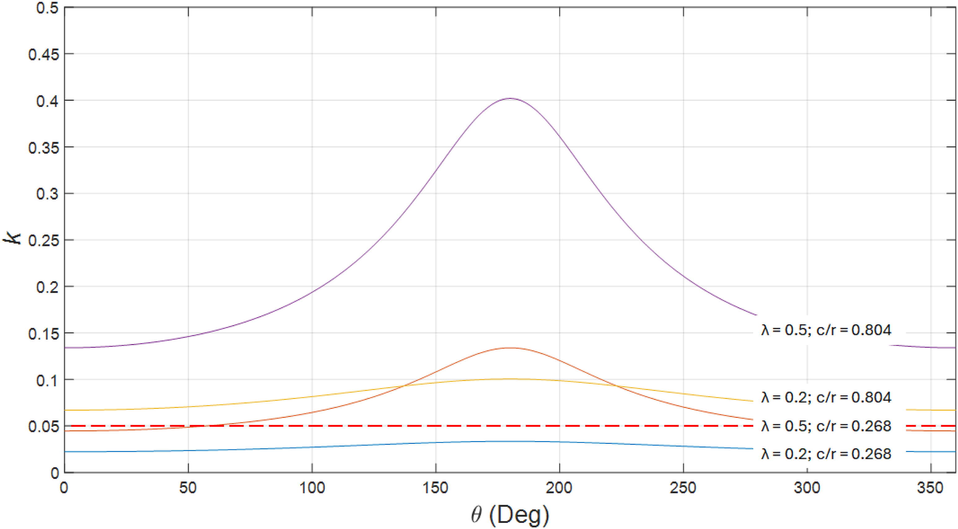$- θ$ displaying the effect of c/r. For c/r = 0.804 blades enter dynamic stall earlier (lower λ) than c/r = 0.268. As c/r increases the blade is more prone to the effect of dynamic stall. The red dashed line is 0.05, below which the blade is not sensitive to pitch rate (Maître et al., 2013).

The preceding analysis infers that larger c/r can contribute to mitigating torque dip by two mechanisms, namely, increasing pitch rate and leveraging the continuously changing virtual camber, ‘virtual morphing’. Both these improve lift in the lift zone and drag in the drag zone and hence torque during start-up phase.

As shown the self-starting capability of turbine with the same solidity could be enhanced by increasing c/r. This means the number of blades is reduced. For example, 3-blade turbine with c/r = 0.268 may be reconfigured to 1-blade turbine with c/r = 0.804. It should be cautioned that 1-blade turbine is prone to poor starting (Dominy et al., 2007). This can be overcome by minor design alteration of the rotor by staggering one-blade sections as shown in Figure 21 (Kirke 2020). It must be noted that blade aspect ratio will reduce which could give rise to tips losses and reduce overall performance. This should be subject of future research.

Figure 21.

Artist impression of the comparison of HDT of identical solidity with three blades (lower c/r) and one blade (higher c/r).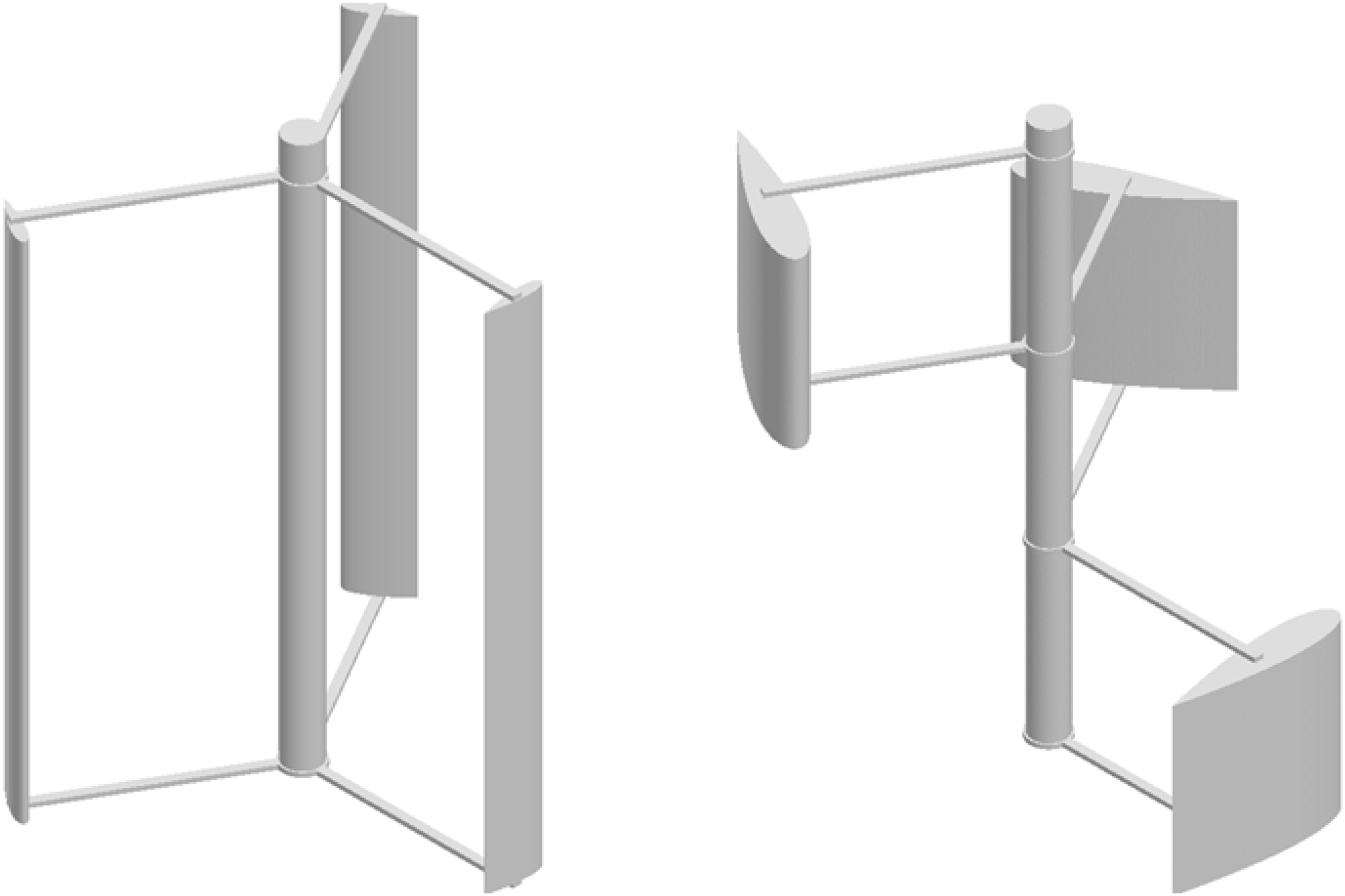

Conclusion

This paper demonstrates that the torque produce by HDT blade is sensitive to the ratio of the chord to the radius, c/r. Turbines with identical $σ = 0.128$ but different c/r = 0.268 and 0.804 are compared. The observed differences in the torque are attributed to: (i) amplification of the variation of incidence angle along blade chord, effectively acting as aerofoil-camber morphing, and (ii) high blade pitch rate effect, especially at low λ (<1) where intra-cycle pitching is significant. The variation of torque over a cycle is related to cyclically unsteady flow field around the blades of HDT with intermittent leading-edge and trailing-edge vortices formation and convection. The finding provides insights into around the blade flow field and torque generation mechanism. The paper highlights the sensitivity of torque production with c/r, offering turbine designers a potential way to improve start-up performance by leveraging virtual morphing phenomena using c/r as target design parameter.

Footnotes

Acknowledgement

An earlier version of this manuscript was shared as a preprint at: .

ORCID iD

Buyung Kosasih

Author Contributions

AJ contributed to the conceptualisation, analysis, and manuscript writing. BK contributed to the conceptualisation, analysis, and manuscript writing. MS contributed to the conceptualisation, the simulations, analysis, and manuscript writing.

Funding

The authors received no financial support for the research, authorship, and/or publication of this article.

Declaration of conflicting interests

The authors declared no potential conflicts of interest with respect to the research, authorship, and/or publication of this article.

Data Availability Statement

The datasets generated or analysed during the present study are available from the corresponding author upon reasonable request.*

References

Abdolahifar

Karimian

SMH

(2022) A comprehensive three-dimensional study on Darrieus vertical axis wind turbine with slotted blade to reduce flow separation. Energy 248: 123632.

Alaimo

Esposito

Messineo

, et al. (2015) 3D CFD analysis of a vertical axis wind turbine. Energies 8(4): 3013–3033.

Ansys

(2023) ANSYS FLUENT 12.0/12.1 documentation 08 11. https://www.afs.enea.it/project/neptunius/docs/fluent/index.htm

Arab

Javadi

Anbarsooz

, et al. (2017) A numerical study on the aerodynamic performance and the self-starting characteristics of a Darrieus wind turbine considering its moment of inertia. Renewable Energy 107: 298–311.

Asr

Nezhad

Mustapha

, et al. (2016) Study on start-up characteristics of H-Darrieus vertical axis wind turbines comprising NACA 4-digit series blade airfoils. Energy 112: 528–537.

Balduzzi

Bianchini

Maleci

, et al. (2014) Blade design criteria to compensate the flow curvature effects in h-darrieus wind turbines. Journal of Turbomachinery 137(1): 2014.

Bangga

Dessoky

Lutz

, et al. (2019) Improved double-multiple-streamtube approach for H-Darrieus vertical axis wind turbine computations. Energy 182: 673–688.

Bhuyan

Biswas

(2014) Investigations on self-starting and performance characteristics of simple H and hybrid H-Savonius vertical axis wind rotors. Energy Conversion and Management 87: 859–867.

Bianchini

Balduzzi

Rainbird

, et al. (2015) On the influence of virtual camber effect on airfoil polars for use in simulations of Darrieus wind turbines. Energy Conversion and Management 106: 373–384.

10.

Botero

Ratkovich

Lain

, et al. (2022) Synthetic jets as a flow control device for performance enhancement of vertical axis hydrokinetic turbines: a 3D computational study. Heliyon 8(8): e10017.

11.

Castelli

Englaro

Benini

(2011) The Darrieus wind turbine: proposal for a new performance prediction model based on CFD. Energy 36(8): 4919–4934.

12.

Celik

Ingham

, et al. (2020) Aerodynamic investigation of the start-up process of H-type vertical axis wind turbines using CFD. Journal of Wind Engineering and Industrial Aerodynamics 204: 104252.

13.

Celik

Ingham

, et al. (2022) Design and aerodynamic performance analyses of the self-starting H-type VAWT having J-shaped aerofoils considering various design parameters using CFD. Energy 251: 123881.

14.

Dominy

Lunt

Bickerdyke

, et al. (2007) Self-starting capability of a Darrieus turbine. Proceedings of the Institution of Mechanical Engineers, Part A: Journal of Power and Energy 221(1): 111–120.

15.

(2016) Numerical and Experimental Investigations of Darrieus Wind Turbine Start-up and Operation. Durham University.

16.

Ebert

Wood

(1997) Observations of the starting behaviour of a small horizontal-axis wind turbine. Renewable Energy 12(3): 245–257.

17.

Hao

Tang

, et al. (2026) Correction for two-dimensional CFD models of vertical axis wind turbines considering the blade tip vortex effect. Renewable Energy 256: 124640.

18.

Hill

Dominy

Ingram

, et al. (2009) Darrieus turbines: the physics of self-starting. Proceedings of the Institution of Mechanical Engineers, Part A: Journal of Power and Energy 223(1): 21–29.

19.

Holst

Church

Wegner

, et al. (2019) Experimental analysis of a NACA 0021 airfoil under dynamic angle of attack variation and low reynolds numbers. Journal of Engineering for Gas Turbines & Power 141(3): 031020.

20.

Hosseini

Goudarzi

(2019) Design and CFD study of a hybrid vertical-axis wind turbine by employing a combined Bach-type and H-Darrieus rotor systems. Energy Conversion and Management 189: 49–59.

21.

Jumper

Schreck

Dimmick

(1987) Lift-curve characteristics for an airfoil pitching at constant rate. Journal of Aircraft 24(10): 680–687.

22.

Keisar

De Troyer

Greenblatt

(2020) Concept and operation of a wind turbine driven by dynamic stall. AIAA Journal 58(6): 2370–2376.

23.

Keisar

Arava

Greenblatt

(2024) Dynamic-stall-driven vertical axis wind turbine: an experimental parametric study. Applied Energy 365: 123199.

24.

Kirke

(2020) Hydrokinetic turbines for moderate sized rivers. Energy for Sustainable Development 58: 182–195.

25.

Kirke

(2024) Towards more cost-effective river hydrokinetic turbines. Energy for Sustainable Development 78: 101370.

26.

Kirke

Lazauskas

(2011) Limitations of fixed pitch Darrieus hydrokinetic turbines and the challenge of variable pitch. Renewable Energy 36(3): 893–897.

27.

Kong

Zhou

Sun

(2024) Improvement of self-starting and power extraction performance of an H-type vertical-axis hydrokinetic turbine by partial deflection of its blades. Ocean Engineering 296: 116855.

28.

Le Fouest

Mulleners

(2024) Optimal blade pitch control for enhanced vertical-axis wind turbine performance. Nature Communications 15(1): 2770.

29.

Le Fouest

Fernex

Mulleners

(2023) Time scales of dynamic stall development on a vertical-axis wind turbine blade. Flowline 3: E11.

30.

Lissaman

PBS

(1983) Low-Reynolds-number airfoils. Annual Review of Fluid Mechanics 15: 223–239.

31.

Liu

Shi

(2016) Numerical study on self-starting performance of Darrieus vertical axis turbine for tidal stream energy conversion. Energies 9(10): 789.

32.

Maalouly

Souaiby

ElCheikh

, et al. (2022) Transient analysis of H-type vertical axis wind turbines using CFD. Energy Reports 8: 4570–4588.

33.

Maître

Amet

Pellone

(2013) Modeling of the flow in a Darrieus water turbine: wall grid refinement analysis and comparison with experiments. Renewable Energy 51: 497–512.

34.

Mannion

Leen

Nash

(2020) Development and assessment of a blade element momentum theory model for high solidity vertical axis tidal turbines. Ocean Engineering 197: 106918.

35.

Masson

Leclerc

Paraschivoiu

(1998) Appropriate dynamic-stall models for performance predictions of VAWTs with NLF blades. International Journal of Rotating Machinery 4(2): 129–139.

36.

Migliore

Wolfe

Fanucci

(1980) Flow curvature effects on Darrieus turbine blade aerodynamics. Journal of Energy 4(2): 49–55.

37.

Mohamed

Elbaz

AMR

Bianchini

(2021) A better insight on physics involved in the self-starting of a straight-blade Darrieus wind turbine by means of two-dimensional computational fluid dynamics. Journal of Wind Engineering and Industrial Aerodynamics 218: 104793.

38.

Peng

Liu

Yang

(2021) A review on the wake aerodynamics of H-rotor vertical axis wind turbines. Energy 232: 121003.

39.

Polagye

Strom

Ross

, et al. (2019) Comparison of cross-flow turbine performance under torque-regulated and speed-regulated control. Journal of Renewable and Sustainable Energy 11(4): 044501.

40.

Rezaeiha

Montazeri

Blocken

(2018) Towards accurate CFD simulations of vertical axis wind turbines at different tip speed ratios and solidities: guidelines for azimuthal increment, domain size and convergence. Energy Conversion and Management 156: 301–316.

41.

Saemian

Bergada

(2025) Active flow control actuators on wind turbines; comprehensive review. Ocean Engineering 339: 121991.

42.

Sagharichi

Maghrebi

Arabgolarcheh

(2016) Variable pitch blades: an approach for improving performance of Darrieus wind turbine. Journal of Renewable and Sustainable Energy 8(5): 053305.

43.

Sun

Zhang

, et al. (2022) Influence of blade numbers on start-up performance of vertical axis tidal current turbines. Ocean Engineering 243: 110314.

44.

Tigabu

Khalid

MSU

Wood

, et al. (2022) Some effects of turbine inertia on the starting performance of vertical-axis hydrokinetic turbine. Ocean Engineering 252: 111143.

45.

Worasinchai

(2012) Small Wind Turbine Starting Behaviour. Durham: PhD thesis.

46.

Worasinchai

Ingram

Dominy

(2016) The physics of H-Darrieus turbine starting behavior. Journal of Engineering for Gas Turbines & Power 138(6): 062605.

47.

Zare Chavoshi

Ebrahimi

(2022) Plasma actuator effects on the flow physics of dynamic stall for a vertical axis wind turbine. Physics of Fluids 34(7): 075131.

48.

Zare Chavoshi

Ebrahimi

(2024) Self-starting and performance improvement of a Darrieus type wind turbine using the plasma actuator. Physics of Fluids 36(5): 055127.

49.

Zhu

Hao

, et al. (2019) Application of flow control strategy of blowing, synthetic and plasma jet actuators in vertical axis wind turbines. Aerospace Science and Technology 88: 468–480.

Leveraging blade virtual morphing to enhance torque during start-up of H-Darrieus turbines

Abstract

Keywords

Introduction

Computational fluid dynamics procedure

Governing equations and turbulence model

The geometry of H-Darrieus turbine and the simulation domain size

The mesh set-up and mesh independence of CFD solution

The time-step set-up

Result and discussion

Comparison of coefficient of performance, C p

Comparison of torque variation per revolution and the flow field correlation

Variable pitched rate and virtual morphing–based explanation

Conclusion

Footnotes

Acknowledgement

ORCID iD

Author Contributions

Funding

Declaration of conflicting interests

Data Availability Statement

References

Comparison of coefficient of performance, C_p