Sage Journals: Discover world-class research

Abstract

One of the key issues in the efficient conversion of wind kinetic energy into electricity is the regulation of turbine speed to achieve maximum electrical power generation. The asynchronous generator with full load double AC-DC-AC power converter has not been widely used due to its poor performance in low wind speed. In this paper a method for turbine speed control of induction generator with full-scale double AC-DC-AC power converter to maximize absorbed wind power in the wide wind speed range, using the calculated maximum turbine power as a reference, is proposed. The configuration of an AC-DC-AC converter for connecting an asynchronous generator to the grid, as well as modeling of Pulse Width Modulation converter is presented in detail. Performance of the proposed control concept to maximize the absorbed wind power is verified through the simulation in MATLAB^®. Finally, the advantages and disadvantages of the proposed control concept are discussed.

Keywords

Wind turbine asynchronous generator speed control pulse width modulation AC-DC-AC converter power quality

Introduction

Wind turbine generators in addition to photovoltaic (PV) power plants, represent the most widespread form of renewable energy applications today. One of the major issues with the use of wind turbines (WT) is the stochastic and intermittent nature of wind as the primary source of energy. Special problem is the speed control of the WT to achieve maximum electrical power generation.

The method of controlling the speed of the WT generator depends largely on the way the generator is connected to the grid. Accordingly, there are: (1) directly connected induction generators to the grid with constant speed, (2) wound rotor induction generator with variable rotor resistance, (3) double-feed induction generators (DFIG) with variable speed, and (4) full converter interfaced synchronous or induction generator with variable speed.

As far as variable-speed generation is concerned, it is necessary to produce constant-frequency electric power from a variable-speed source. This can be achieved by means of synchronous generators, provided that a static frequency converter is used to interface the machine to the grid. Using a wound-rotor induction generator fed with variable frequency rotor voltage allows fixed-frequency electric power to be extracted from the generator stator. One of the main advantages of DFIG with variable speed is that, if rotor current is governed applying stator-flux-oriented vector control, carried out using double-sided PWM inverters, decoupled control of stator side active and reactive powers results. However, there are some disadvantages of DFIG configurations such as: (1) regular maintenance of slip ring and brush assembly in nacelle, (2) limited fault ride-through and voltage regulation capability, (3) rotor and gearbox stresses during system unbalanced faults, (4) large short circuit contribution, (5) interactions between grid and generator; susceptible to sub synchronous interaction, etc.

The full scale converter interfaced generator with variable speed has many advantages such as: (1) maximum flexibility—fully controllable converter interface, (2) decoupled control of active power and voltage regulation, (3) controllable short circuit contribution, (4) theoretically infinite duration low-voltage ride-through capability, (5) no exposure to system faults for generator, gearbox (in geared systems), (6) reactive capability curve which is similar to synchronous machines, (7) no slip rings; easy maintenance, and (8) self-synchronizing; no supplemental equipment or capacitors required. Possible disadvantages of full converter interfaced generator is limited (but controllable) fault current contribution, therefore it may require sophisticated collector protection.

The wind turbine generator control has been in the research focus in last two decades. The references (Abuaisha, 2014; Araghi et al., 2020; Bechir et al., 2012; Behnkel and Muljadi, 2005; Cardenas and Pena, 2004; Deshpande et al., 2018; Divya and Rao, 2006; Ekanayake et al., 2003; Inthamoussou et al., 2016; Jiao et al., 2005; Ledesma and Usaola, 2005; Mansouri et al., 2004; Martins et al., 2007; Mei et al., 2012; Mérida et al., 2014; Mihet-Popa et al., 2004; Rawn et al., 2006; Slootweg et al., 2003; Tapia et al., 2003, 2006; Trudnowski et al., 2004; Yin et al., 2016) analyze dynamic modeling of wind turbine generator and this issue can be classified in several topics: modeling presentation, modeling simplification, modeling comparison, and wind farm equivalent modeling. The model and dynamics of the wind turbine connected to an infinite power network is studied (Mansouri et al., 2004). Ledesma and Usaola (2005) presents a dynamic model of DFIG on the assumption that the current control does not influence the transient stability. The model of DFIG is analyzed as a hybrid asynchronous and synchronous machine (Jiao et al., 2005). Dynamic modeling of DFIG wind turbines is presented in Ekanayake et al. (2003). The reduced model for variable-speed WT with synchronous generator and full power conversion topology is presented in Behnkel and Muljadi (2005). Validation of the fixed speed WT dynamic models with measured data is presented in Martins et al. (2007). A general model for representing the variable speed WT in power system dynamics simulations is presented in Slootweg et al. (2003). The research into the limits on controllable power output from wind energy conversion systems with a fully rated converter interfaced WT is presented in Rawn et al. (2006). In Bechir et al. (2012) a wind energy conversion system with full-scale power converter and squirrel cage induction generator is presented. It is demonstrated that the full-scale power converter configuration has ability to remain in synchronism during and after major voltage sags and the capability to keep power quality.

Mei et al. (2012) investigated configuration uses a squirrel-cage induction generator connected to the grid through a back-to-back double Pulse Width Modulation (PWM) converter. The generator side adopted vector control technology of the rotor slip frequency, and the grid side used the network voltage-oriented control and voltage and current dual close-loop control strategy.

The models for WT generating systems and their application in the load flow studies are presented in Divya and Rao (2006). Evaluation of the wind farm active and reactive power performances is reported in Tapia et al. (2006). The fixed-speed wind-generator and the wind-park modeling for transient stability studies are presented in Trudnowski et al. (2004). Modeling and control of the WT driven DFIG is reported in Tapia et al. (2003) with the objective to control a DFIM power factor. It is known that the ability to generate electricity with power factors different to one would reduce the costs of introducing additional capacitors for reactive power regulation.

Vector control of the induction machines for variable-speed wind energy applications using sensor less technology is presented in Cardenas and Pena (2004). In this approach the sensor less control system is based on a model reference adaptive system (MRAS) observer to estimate the rotational speed from the rotor slot harmonics using an algorithm for spectral analysis.

A WT generator modeling where rotational speed is the controlled variable is presented in Mihet-Popa et al. (2004) including soft-starter start-up and power-factor compensation. Output power maximization of wind energy conversion system using doubly fed induction generator and applying Maximum Power Point Tracking (MPPT) algorithm, as well as its laboratory setup is presented in Deshpande et al. (2018).

In Abuaisha (2014) generic models for variable speed WT and generator/converter subsystem are implemented. Active power control of WT covering the complete wind speed range and extreme event loads is proposed in Inthamoussou et al. (2016). Yin et al. (2016) is demonstrated that increased power capture and enhanced overall efficiency can be achieved by using a hydro-viscous transmission based maximum power extraction control. The power optimization problem solution in WT without wind speed measurements using slide mode control is proposed in Mérida et al. (2014). An economic nonlinear model predictive control of WT to enhance net energy capture applying wind speed forecasting is proposed in Araghi et al. (2020). A solution to reduce overheating and increase WT systems availability is proposed in Singh et al. (2021).

Despite numerous advantages the asynchronous generator with full load power converter has not been widely used mainly due to its poor performance in low wind speed, which then requires a gear box with high gear ratio. The aim of study presented in this paper is to analyze the control of WT induction generator with full load power converter to maximize absorbed wind power and improve its power transfer performance. In this paper a concept of speed control of the WT asynchronous generator connected to the grid via a double AC-DC-AC PWM converter, using the calculated maximum turbine power as a reference, is applied (Pesut and Ciric, 2020).

The main contribution of the paper is developing and testing a comprehensive model of a new speed controller to maximize absorbed wind power in the wide wind speed range, and to improve the induction generator real and reactive power transfer performance applying the average and the switching model of PWM converter. The performance of the proposed drive control concept is verified through the simulation on the model developed in MATLAB^®. Besides, the advantages and disadvantages of the control concept as well as the power quality performance of the asynchronous generator with full-scale double AC-DC-AC power converter configuration is analyzed and discussed.

Model of energy converter

The speed control of generator is performed to control the speed of the wind turbine. For each wind speed, there is an optimum point, that is, the optimal turbine speed for which the maximum wind power is captured. The information on this operating point is known from equation (1) (Pesic, 1994). By knowing the turbine radius R_tur and the optimum value of tip speed ratio λ_opt, the reference speed of the WT can be obtained based on the measurement of wind speed V_wind. This value could be used as a reference in the speed control loop. However, this method is not of practical use because of the problems encountered in measuring wind speed such as the measurement inaccuracy and the problem of instrument placement.

One way of overcoming the above-mentioned problem is to realize the speed control by calculating the maximum power of the WT P_max. Figure 1 shows the power diagrams of a WT for two wind speeds. If it is assumed that the WT speed is such that the drive is stationary at a wind speed that is less than nominal one, the operating point will be at point A, therefore the turbine will capture maximum wind power at that speed. In case of increased wind speed, there is a jump in the setpoint at the point B. When switching to a new characteristic, the power factor of the turbine C_p=P_out/P_in is no longer at the optimum point as can be seen from the equation (1), therefore the WT power is no longer maximal for this new wind speed (Maxime, 2000). The mechanism of the turbine reaching the optimal point is based on a comparison of the calculated WT power in the optimum point (equation (2)), and the actual turbine power at that point, which is obtained by the metering power in the DC-bus, P_dc (equation (3)), and adding the generator losses P_g calculated in equation (4) (Maxime, 2000):

λ = \frac{R_{tur} \cdot ω_{tur}}{V_{wind}}

(1)

P_{\max} = \frac{1}{2 \cdot λ_{opt}^{3}} \cdot C_{p} (λ_{opt}) \cdot ρ \cdot R_{tur}^{5} \cdot π \cdot ω_{tur}^{3}

(2)

P_{dc} = U_{dc} \cdot i_{isp}

(3)

P_{g} = R_{s} \cdot i_{s}^{2} + R_{r} \cdot i_{r}^{2} + P_{Fe}

(4)

Figure 1.

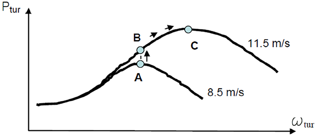
Movement of the turbine operating point when changing wind speed.

where

λ is tip speed ratio of wind turbine,

C_p is power factor of wind turbine (C_p = P_out/P_in), Figure 2,

ω_tur is angle rotation speed of the turbine,

V _wind is wind speed,

ρ is air density,

U _dc is voltage of the DC bus,

i _isp is current of the DC bus to the rectifier,

R_s and R_r is stator and rotor resistance,

i_s and i_r is stator and rotor current, and

P_Fe is iron loss.

Figure 2.

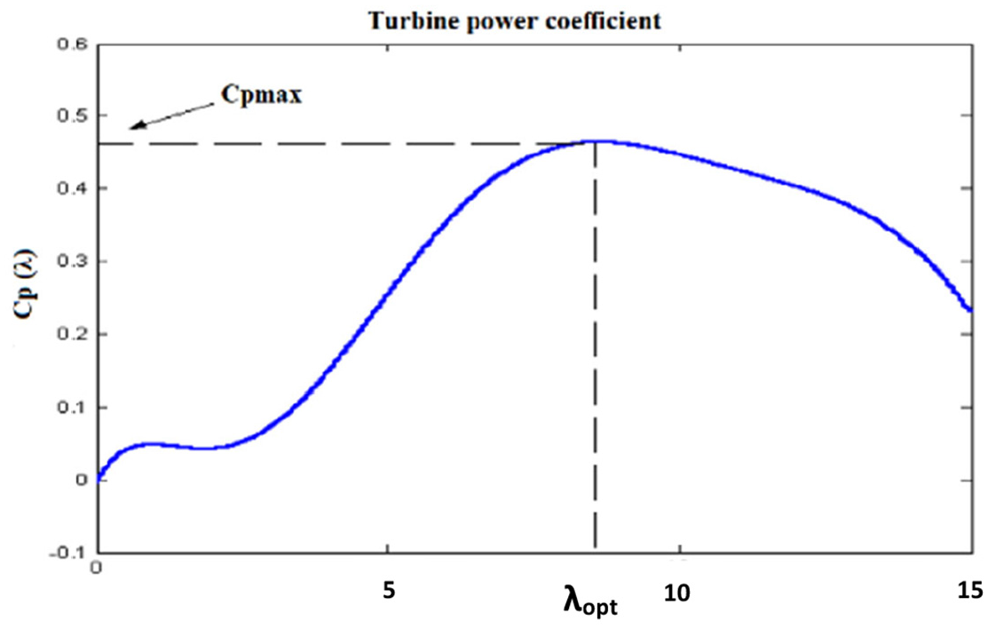
Wind turbine power factor.

After the jump of the operating point to the point B, the tip speed ratio λ and the power factor of the turbine C_p decreased, but the power of the turbine is higher than before the change in wind speed. As the power of the WT increased for the same speed, the torque of the WT increased, therefore the drive accelerates, and the operating point moves toward point C.

The higher value of maximum WT power due to the increased speed is calculated based on the equation (2). Deduction the sum of powers P_dc and P_g from the maximum WT power gives an error at the input of the speed controller. The output of this controller provides a reference for a torque regulator which, based on the error of the input of the speed controller, increases the reference of the q-axis stator current i_{sq_ref}. In this way, the generator increases the conversion torque, which is opposed to the increased WT torque.

The converter configuration with IGBT transistors is shown in Figure 3. Modern IGBT transistors have voltage rating from 4.5to 6.5 kV, and withstanding currents from 250 A to as much as 1200 A.

Figure 3.

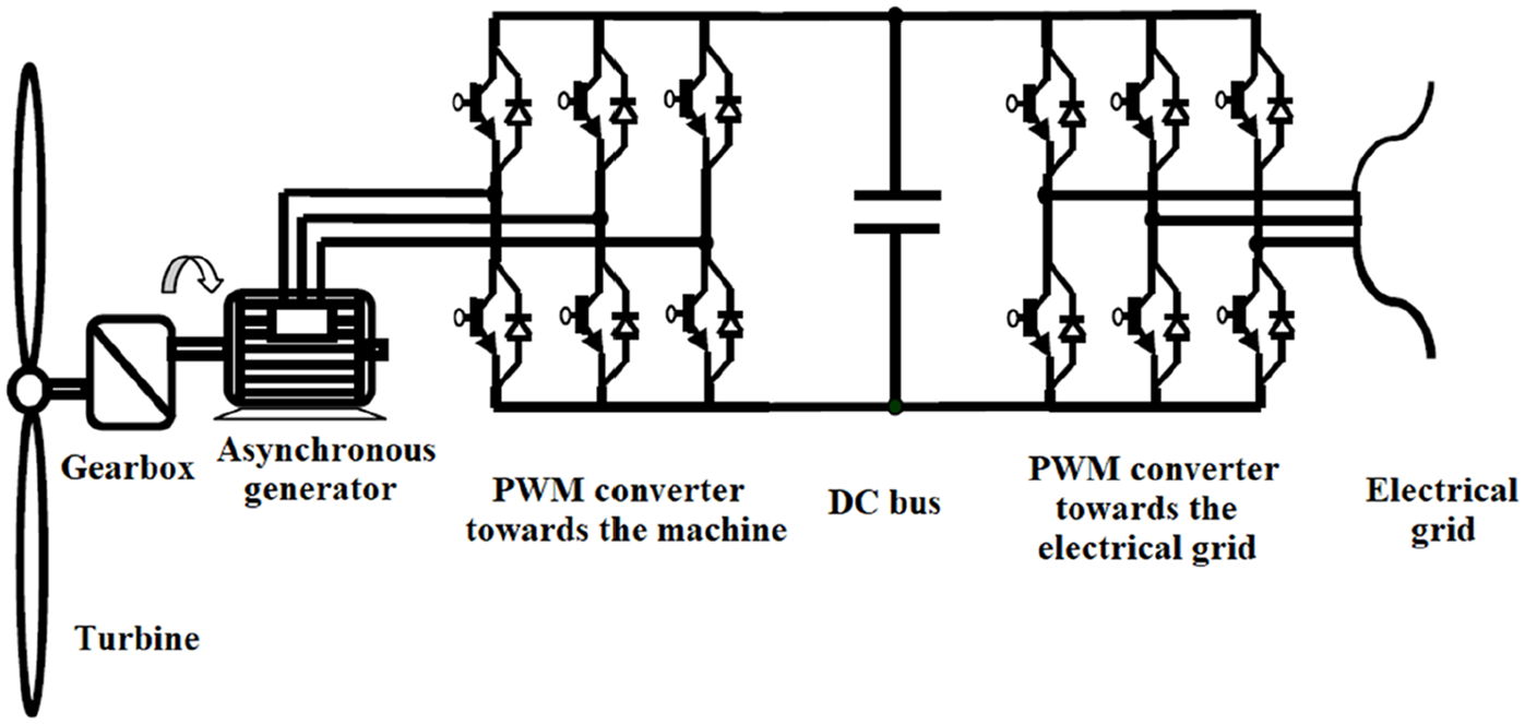
Asynchronous generator connected to the mains via double AC-DC-AC PWM converter.

The torque on the turbine shaft is transmitted to the shaft of the asynchronous generator by the gearbox, which increases the input speed. By controlling the PWM converter from the generator side according to an algorithm that provides control of the space vector of the generator flux (vector control), it is possible to directly control the torque of the generator conversion.

Since the vector control involves knowing the frequency of the stator variables, it is necessary to know the rotation speed of the turbine in which the wind power absorption is maximized. This speed corresponds to the sliding at which the maximum absorption of wind energy is achieved. By controlling the PVM converter toward the generator from the DC voltage of the DC bus, a voltage of a certain frequency is obtained, creating a torque that equals the torque of the WT exactly at the speed at which the maximum efficiency of the turbine circuit is provided.

The DC-bus voltage control ensures that all energy from the generator is forwarded to the grid. By controlling the PWM converter, it is possible to control the phase position between the voltage and the current of the grid, which in addition to control of active power flow regulates the reactive power flow as well. Block diagram of asynchronous generator speed control is shown on Figure 4.

Figure 4.

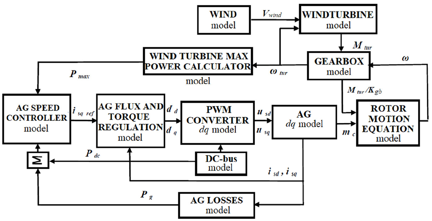
Block diagram of asynchronous generator speed control.

The power of three-blade WT is represented by the equations (5) and (6) (Pesic, 1994),

P_{turbine} = C_{p} (λ) \cdot P_{wind}

(5)

P_{turbine} = \frac{1}{2} \cdot C_{p} (λ) \cdot ρ \cdot R_{turbine}^{2} \cdot π \cdot V_{wind}^{2}

(6)

The input variables in the WT simulation model are turbine speed and wind speed, while the output variable is the torque on the turbine shaft. In this approach, the nominal mechanical angular rotational speed of the generator is taken as the input speed, and the output speed is the nominal rotational speed of the WT. Accordingly, the mathematical model of the gearbox is defined by the transmission relation given by gear ratio K_red (equation (7)),

K_{red} = \frac{ω_{n}}{ω_{tur}} = \frac{\frac{ω_{s} + ω_{kl}}{p}}{ω_{tur}}

(7)

where

ω_n is rated generator angular rotational speed,

ω_s is synchronous angular rotational speed,

ω_kl is the nominal angular rotational speed of the slip,

ω_tur is nominal rotational speed of the turbine, and,

p is number of pair of poles of the generator.

The motion equation is set for the asynchronous generator shaft and is given by the equation (8) (Pesic, 1994).

(J_{AG} + \frac{J_{tur}}{K_{red}^{2}}) \cdot \frac{d ω}{dt} = p \cdot m_{c} - \frac{M_{tur}}{K_{red}}

(8)

where

J_AG is the torque of inertia of induction generator,

J_tur is the torque of inertia of the turbine, and,

m_c is the conversion torque.

Generator control

All three regulators are implemented in analog technique and have PI (proportional integral) effect. The PI controller achieves a trade-off between the two good features of a PI controller, namely the speed of action of the P controller and the complete elimination of static error in the I controller. The dynamic behavior of the PI controller is described by equation (9) (Vukosavic, 2010), (Gitano-Briggs 2010).

y (t) = K_{p} \cdot [e (t) + \frac{1}{T_{i}} \int_{0}^{t} e (t) \cdot dt]

(9)

where e(t) is the controller input, or the error and y(t) is the controller output.

In the state space, the controller characteristics are expressed by the transfer function G_Pi given by the equation (10),

G_{PI} (s) = K_{p} \cdot (1 + \frac{1}{s \cdot T_{i}}) = K_{p} + \frac{1}{s} \cdot K_{i}

(10)

where,

K_p is the coefficient of proportional action,

T_i is the time constant of the integration, and

K_i is the coefficient of integral action.

After averaging (in the switching period) and dq transformation of coordinates, the inverter model is given by equations (11) and (12) (Hiti and Borojevic, 1994),

\frac{d}{dt} [\begin{matrix} i_{d} \\ i_{q} \end{matrix}] = [\begin{matrix} 0 & ω_{s} \\ - ω_{s} & 0 \end{matrix}] \cdot [\begin{matrix} i_{d} \\ i_{q} \end{matrix}] - \frac{R_{mr}}{L_{mr}} \cdot [\begin{matrix} i_{d} \\ i_{q} \end{matrix}] + \frac{1}{L_{mr}} \cdot [\begin{matrix} d_{d_{inv}} \\ d_{q_{inv}} \end{matrix}] \cdot U_{dc} - \frac{1}{L_{mr}} \cdot [\begin{matrix} u_{d} \\ u_{q} \end{matrix}]

(11)

i_{inv} = [\begin{matrix} d_{d_inv} & d_{q_inv} \end{matrix}] \cdot [\begin{matrix} i_{d} \\ i_{q} \end{matrix}]

(12)

where

i_d, i_q, u_d, and u_q are grid current and voltage along the d-q axis, respectively,

d_{d_inv} is fill factor of the voltage u_d,

d_{q_inv} is fill factor of the voltage u_q,

i_inv is current of the DC bus toward the inverter.

By analogy, the averaged model of the rectifier is given by the equations (13) and (14),

[\begin{matrix} u_{sd} \\ u_{sq} \end{matrix}] = [\begin{matrix} d_{d_isp} & 0 \\ 0 & d_{q_isp} \end{matrix}] \cdot U_{dc}

(13)

i_{isp} = [\begin{matrix} d_{d_isp} & d_{q_isp} \end{matrix}] \cdot [\begin{matrix} i_{sd} \\ i_{sq} \end{matrix}]

(14)

where

d_{d_isp} is fill factor of the voltage u_sd,

d_{q_isp} is fill factor of the voltage u_sq, and

i_isp is current of the DC bus toward the rectifier.

DC-bus voltage control

The DC-bus is shown in Figure 5, and for averaged model of PWM converter the rectifier current $i_{isp}$ and the inverter current $i_{inv}$ is given by equations (15) and (16), respectively (Hiti and Borojevic, 1994; Pesic, 1994),

i_{isp} = S_{aN_isp} \cdot i_{sa} + S_{b N_{isp}} \cdot i_{sb} + S_{c N_{isp}} \cdot i_{sc}

(15)

i_{inv} = S_{aN_inv} \cdot i_{a} + S_{b N_{inv}} \cdot i_{b} + S_{c N_{inv}} \cdot i_{c}

(16)

Figure 5.

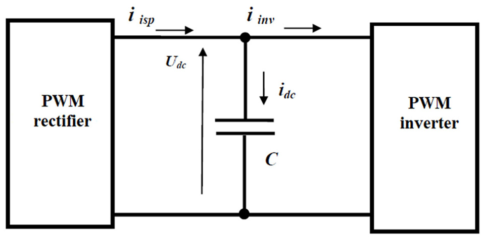
DC-bus.

where

i_sa, i_sb, and i_sc are phase stator currents,

i_a, i_b, and i_c are phase grid currents,

S_{aN_isp}, S_{bN_isp}, S_{cN_isp} are the state of the switches in rectifier branch a, b, and c respectively, and

S_{aN_inv}, S_{bN_inv}, S_{cN_inv} are the state of the switches in inverter branch a, b, and c, respectively.

As the difference to the averaged model, the aim of switching modeling of the PWM converters is obtaining the switching states (S_a, S_b, and S_c) of the branches of the converter bridge including the running time of each switch, as well as the order of their running in the switching period. One of the ways for realization of switching PWM converter model is Space Vector Modulation (SVM) of control signals.

DC bus currents in the switching model of PWM converter are given by equations (17) and (18),

i_{isp} = d_{d_isp} \cdot i_{d} + d_{q_{isp}} \cdot i_{q}

(17)

i_{inv} = d_{d_inv} \cdot i_{d} + d_{q_{inv}} \cdot i_{q .}

(18)

The purpose of DC bus control is to forward all real power that has entered the DC bus to the grid. Namely, when the active power entering the DC bus changes, its voltage also changes, therefore through the voltage control the power flow to the grid can be regulated. The controller input error is the difference between the reference value and the measured DC-bus voltage value, and the output is the reference value for the regulator of active component of the grid current. If the inflow of active power into the DC bus increases (due to an increase in wind speed), the voltage of the DC-bus U_dc also increases. There is now an error at the input of the voltage regulator U_dc, and it responds by increasing the active component of the grid current, thus increasing the power flow to the grid (Figure 4).

As the active power exiting the DC bus increases and the same active power value dictated by the power of the wind enters, the power of the DC bus decreases. This reduction in power of DC-bus is accompanied by a reduction of voltage U_dc. In this way, maintaining the U_dc voltage at the setpoint, it was achieved that all the power received from the generator was forwarded to the grid. To enable regulation, an analog PI controller whose dynamics is given by equation (9) and whose transfer function is given by equation (10), is applied (Hiti and Borojevic, 1994).

Vector control of power flow

Vector control of power flow involves observing the variables of the grid in the d-q coordinate system. Since a power invariant system is applied, the grid power is given by the equation (19) (Vukosavic, 2010),

p = u_{d} \cdot i_{d} + u_{q} \cdot i_{q}

(19)

Grid voltages u_d and u_q cannot be used to control the power flow since the amplitude and frequency of the grid voltage are constant. The reactive power control is realized by the controller of the reactive component of the grid current $i_{d}$ , while the regulation of the real power is enabled by the controller of the active component of the grid current $i_{q}$ . The reference current $i_{d}$ is set to the desired level, while the reference current $i_{q}$ is obtained from the output of the DC-bus voltage regulator (Figure 4).

The outputs of the controller are the values of the fill factors $d_{q_inv}$ and $d_{d_inv}$ , which are used to obtain voltage at the output of the PWM converter and $u_{d_inv}$ . In this way, the grid currents along the d and q axes are actuated, by acting on the voltage, allowing the control of the active and reactive power flow to the grid.

In the stationary coordinate system of the α-β axis shown in Figure 6, the vector of the reference voltage V_ref to be obtained at the output of the converter bridge is of constant amplitude and rotates at an angular velocity $ω_{s} = 2 π f_{s}$ . The eight operating states of the converter bridge consist of two zero vectors and six non-zero vectors, defined by expression (20) (Analog Devices, 2000; Marcetic, 2014),

{\vec{V}}_{k} = \sqrt{\frac{2}{3}} \cdot U_{dc} \cdot e^{j (k - 1) \frac{π}{3}}, k = 1, \dots, 6 .

(20)

Figure 6.

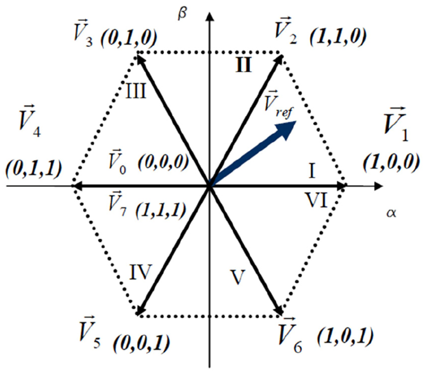
Switch states defined in a stationary coordinate system.

The state vectors form a hexagon divided into six sectors so that the reference vector passes through the marked sectors. The states of the bridge switch are defined by a triple (x, y, z) where x, y, and z define the states in the bridge branches a, b, and c, respectively, and can have the value 0 or 1. In this case, 1 denotes that the upper switch leads to the observed group of bridges, and 0 denotes that the lower switch leads to the branch. As a rule, when the upper bridge switch leads, the lower must not lead and vice versa. Assuming that the signal selection time is short, the vector of the reference voltage lying in sector k can be considered constant in the switching period T_S.

Switching time defined by the state V_k, V_(k+1) in the switching period T_S is given in equations (21) and (22) (Analog Devices, 2000),

(\begin{matrix} T_{k} \\ T_{k + 1} \end{matrix}) = \frac{D \cdot T_{S}}{\sqrt{2}} \cdot (\begin{matrix} \sin (\frac{k π}{3} - θ) \\ - \sin (\frac{(k - 1) π}{3} - θ) \end{matrix})

(21)

D = U_{dc} \cdot \sqrt{d_{d}^{2} + d_{q}^{2}}

(22)

where

U_dc is voltage of the converter bridge,

u_d and u_q are voltage of converter bridge along the d and q axis, given in equation (23),

u_{d} = D_{d} \cdot U_{dc}, u_{q} = D_{q} \cdot U_{dc}

(23)

D_d and D_q are averaged values of switching state of the bridge.

Equation (23) represent the values of the desired voltage at the output of the converter bridge along the d and q axes of the coordinate system that rotates at a synchronous angular velocity. Calculation of inverter reference voltage components along the α and β axes is demonstrated in Figure 7.

Figure 7.

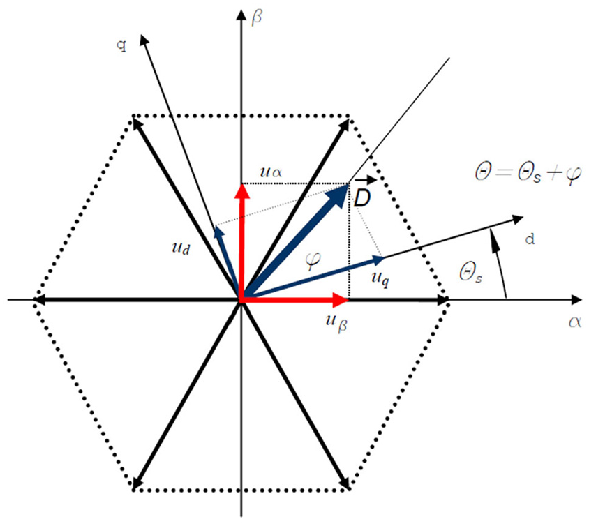
Calculation of inverter reference voltage components along the α and β axes.

Simulation results

The WT induction generator 2 MW of rated power (Appendix) with dual full-scale AC-DC-AC converter with averaged and the switching model of a PWM converter is simulated in MATLAB Simulink^®. It is assumed that the system is stationary at the wind speed of 8.5 m/second whereby the turbine receives maximum wind power, and the coefficient of turbine power is at maximum value (C_pmax=0.465). At the instant t=2 seconds, the wind speed changes to 11.5 m/second, with this being the nominal wind speed, that is, the wind speed at which the turbine gives nominal power.

Simulations on average model of PWM converter

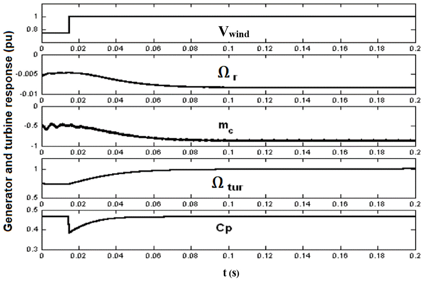
The response of characteristic variables of the generator and WT(in per unit) to changes in wind speed is shown on Figure 8. The diagrams are shown with the normalized values, which are presented in Appendix.

Figure 8.

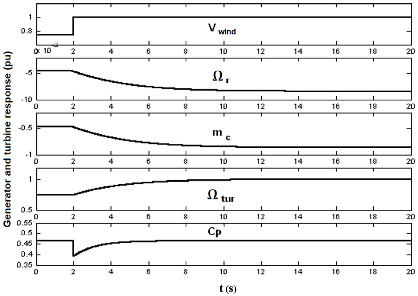
Response of characteristic turbine and generator variables (in per unit) to changes in wind speed, using averaged PWM converter model—V_wind: wind speed; Ω_r = ω_e− ω: slip speed; m_C: conversion torque; Ω_tur: turbine speed; C_p: turbine power factor.

It is observed that as the wind speed increase, the slip of the generator rotor speed increases, as the machine needs to increase the conversion torque m_c, which must counteract the increased wind turbine torque. With the action of the speed controller these torques should be equalized at the speed at which the power capture is maximum at the new wind speed.

This practically means that the wind turbine speed ω_tur must change for the same ratio as the wind speed V_wind, since then the wind turbine power factor C_p will remain at its maximum value. This is confirmed by the simulation, where after the transient process the wind turbine power factor value is again at the maximum, C_p=0.465 (Figure 8).

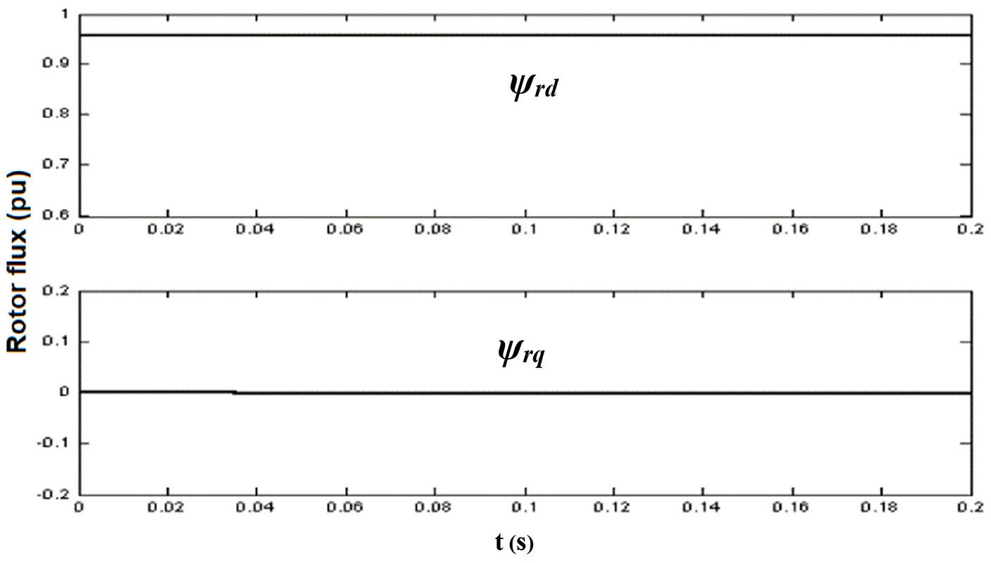
One of the goals of the regulation was the realization of vector control of the asynchronous generator. Figure 9 shows the per unit values of the rotor flux along the transverse and longitudinal rotor axis. The vector control requires that the rotor flux in the transverse axis Ψ_rq is zero, while the flux in the longitudinal axis Ψ_rd provides the nominal excitation of the generator. The diagram shows that the values of flux, on both axes, before and after the resulting change are the same, and they do not change significantly during the transient period, meaning that vector control of the induction generator was realized.

Figure 9.

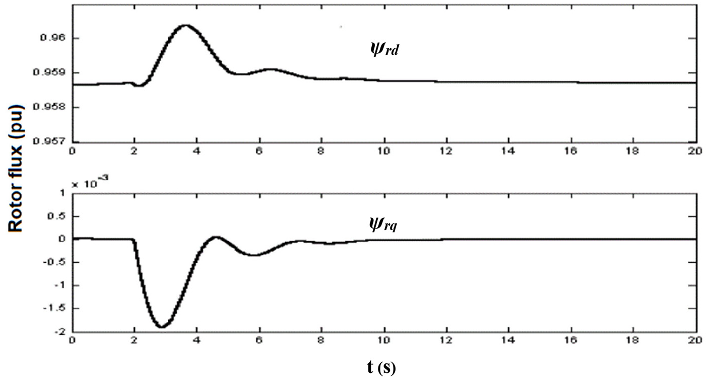
Rotor flux along the longitudinal Ψ_rd and transverse axes Ψ_rq in per unit—average PWM converter model.

Increasing the wind speed resulted in an increase in the torque of the generator, that is, an increase in the generated power. The diagram in Figure 10 shows how increased generated power is transmitted to the grid. An increase in generator power increases the rectifier current i_isp that supply the DC bus. The increasing of rectifier current i_isp results in an increase in the voltage of the DC bus, U_dc. The voltage U_dc starts to increase the reference of the active component of the grid current i_q, resulting in the increase of the injected power into grid. Due to the increased power injected into the grid, the PWM inverter draws more current from the DC bus, i_inv. The current i_q will increase if there is a difference between the reference and actual DC bus voltage. After the transient period, the voltage U_dc is again at its reference value, and the inverter current i_inv increased to the value of the stator current i_s. The power entering the DC bus equals to the output power which was the objective of the speed control. The controller maintains the grid current i_d at zero, therefore only active power is injected into the grid, that is, the power factor equals one.

Figure 10.

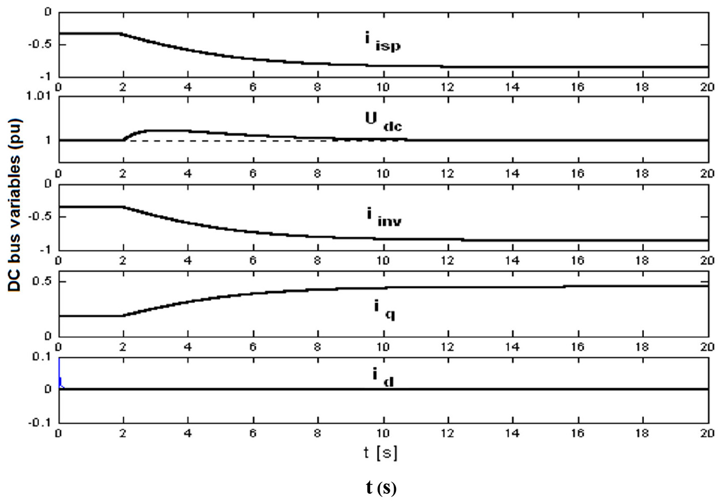
Variable quantities of DC bus and the grid (in per unit)—averaged PWM converter model—i_isp: rectifier current; U_dc: DC bus voltage; i_inv: inverter current; i_q: active component of grid current; i_d: reactive component of grid current.

Figure 11 shows the voltage and current waveforms of phase R of the grid. It is observed that the grid current wave i_a and the voltage wave U_R are in counter-phase, meaning unity power factor.

Figure 11.

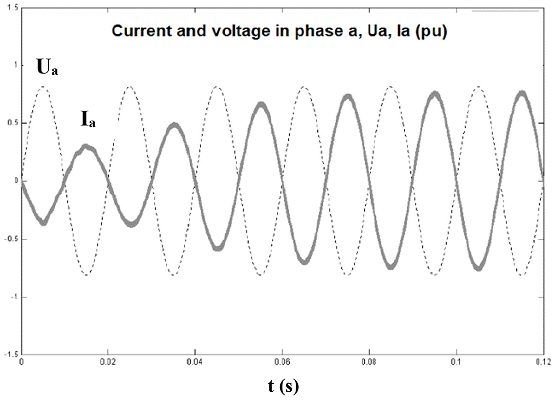
Current and voltage waveform in phase a during transition.

Simulations on switching model of PWM converter

Due to long calculation time, to present the results in shorter time, the simulation of switching model of PWM converter is performed with 100 times less value of drive inertia. In the Figures 12 to 14 the characteristic variables of the drive, in case of switching model of PWM converter are presented.

Figure 12.

Response of characteristic turbine and generator variables (in per unit) to changes in wind speed—switching PWM converter model—V_wind: wind speed; Ω_r = ω_e− ω: slip speed; m_C: conversion torque; Ω_tur: turbine speed; C_p: turbine power coefficient.

Figure 13.

Rotor flux along the longitudinal Ψ_rd and transverse axes Ψ_rq in per unit—switching PWM converter model.

Figure 14.

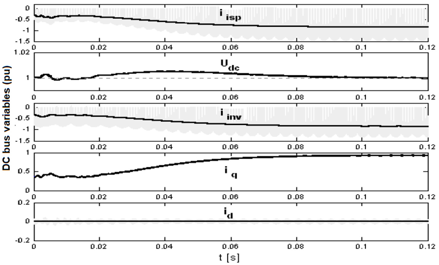
Variable quantities of DC bus and the grid (in per unit)—switching PWM converter model—i_isp: rectifier current; U_dc: DC bus voltage; i_inv: inverter current; i_q: active component of grid current; i_d: reactive component of grid current.

Rotor flux along the longitudinal Ψ_rd axes is kept on the rated value while the rotor flux along the transverse axes Ψ_rq is kept at the zero, meaning the vector control is achieved (Figure 13).

The real value of rectifier current i_isp and inverter current i_inv on the Figure 14 is shown by gray curve while the average value of these currents in switching period T_S is represented by black curve.

Power quality issues

Harmonic distortion (HD) of the grid current and voltage caused by the operation of the PWM inverter is considered in the assessment of power quality. One period of the inverter voltage output (branch a) is shown in Figure 15.

Figure 15.

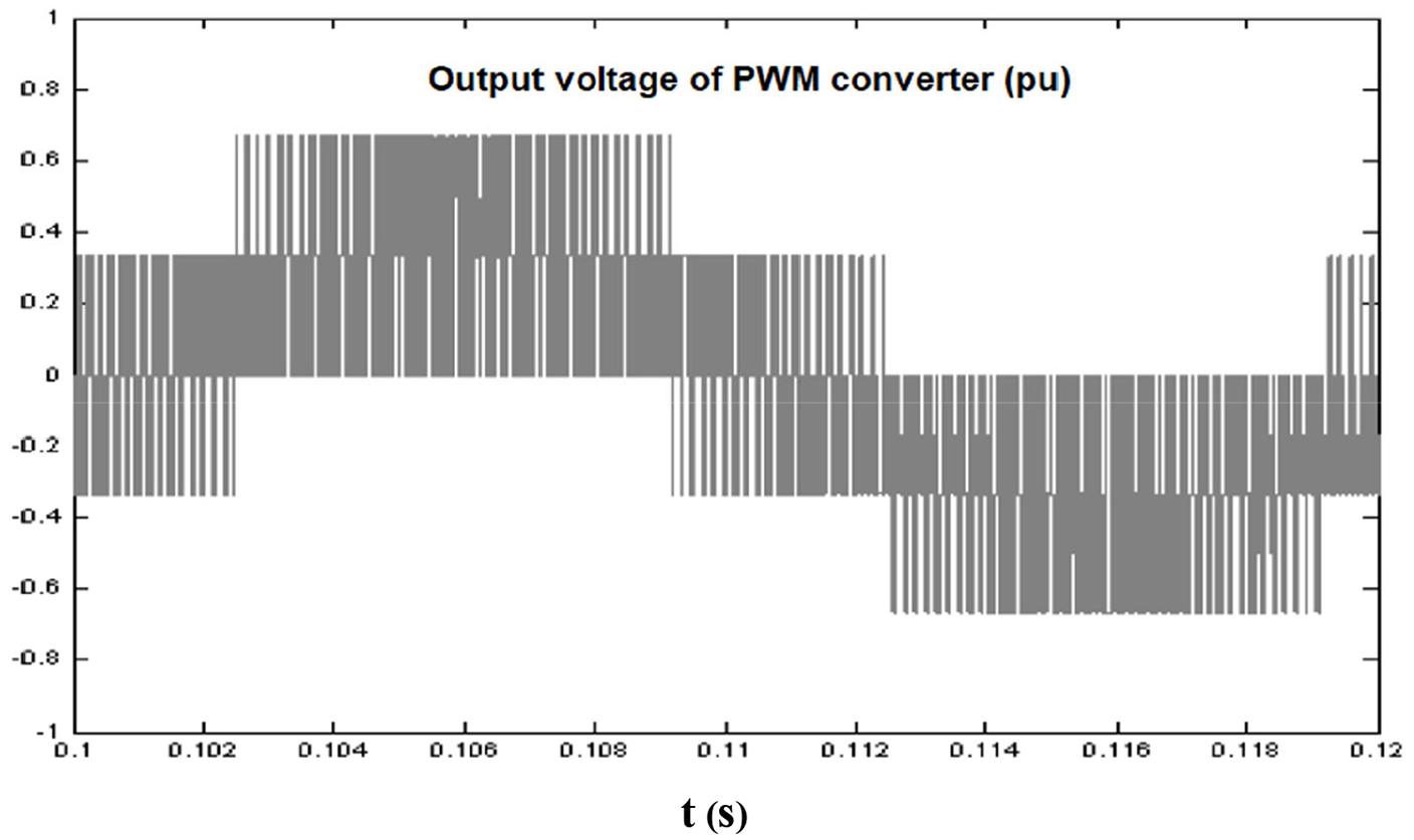
Phase voltage UaN (in p.u.) at the output of the PWM converter.

Figure 16 shows the harmonic distortion of the phase current HDia while the Figure 17 shows harmonic distortion of grid voltage HDUaN. It is observed that the higher harmonics are shifted to the area around the 120th harmonic which corresponds to the switching frequency of the converter bridge (f_S = 6 kHz). That is the advantage of pulse-width modulation of inverter control, since the higher voltage and current harmonics move along the frequency axis. Translating higher harmonics enables their easier filtering, since the filters of smaller values of capacitance and inductance can be applied. However, this increase has its limits because by increasing the power passing through the converter, the switching frequency of the converter bridge must be reduced.

Figure 16.

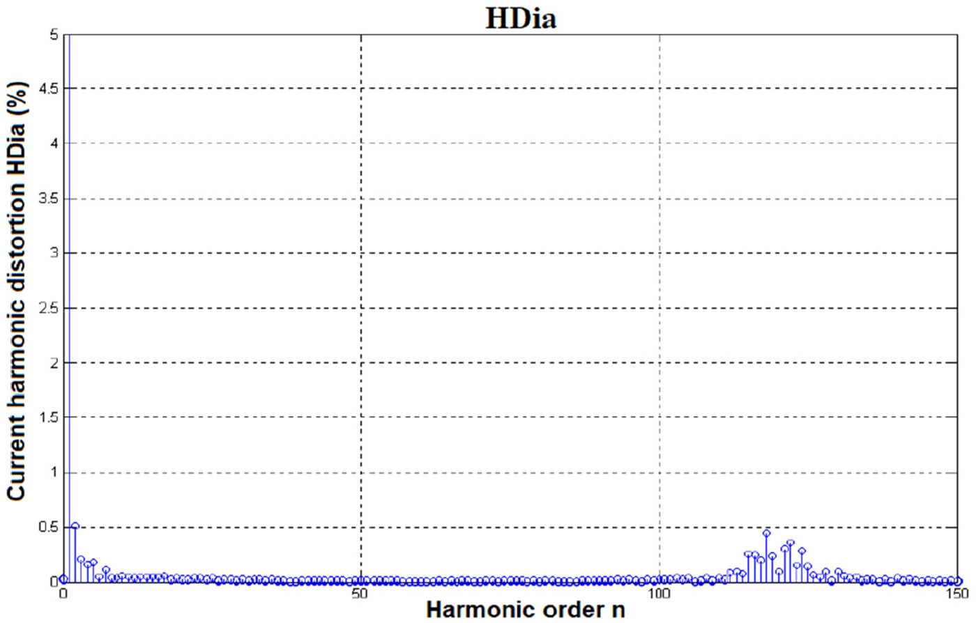
Harmonic distortion of grid current HDia (%).

Figure 17.

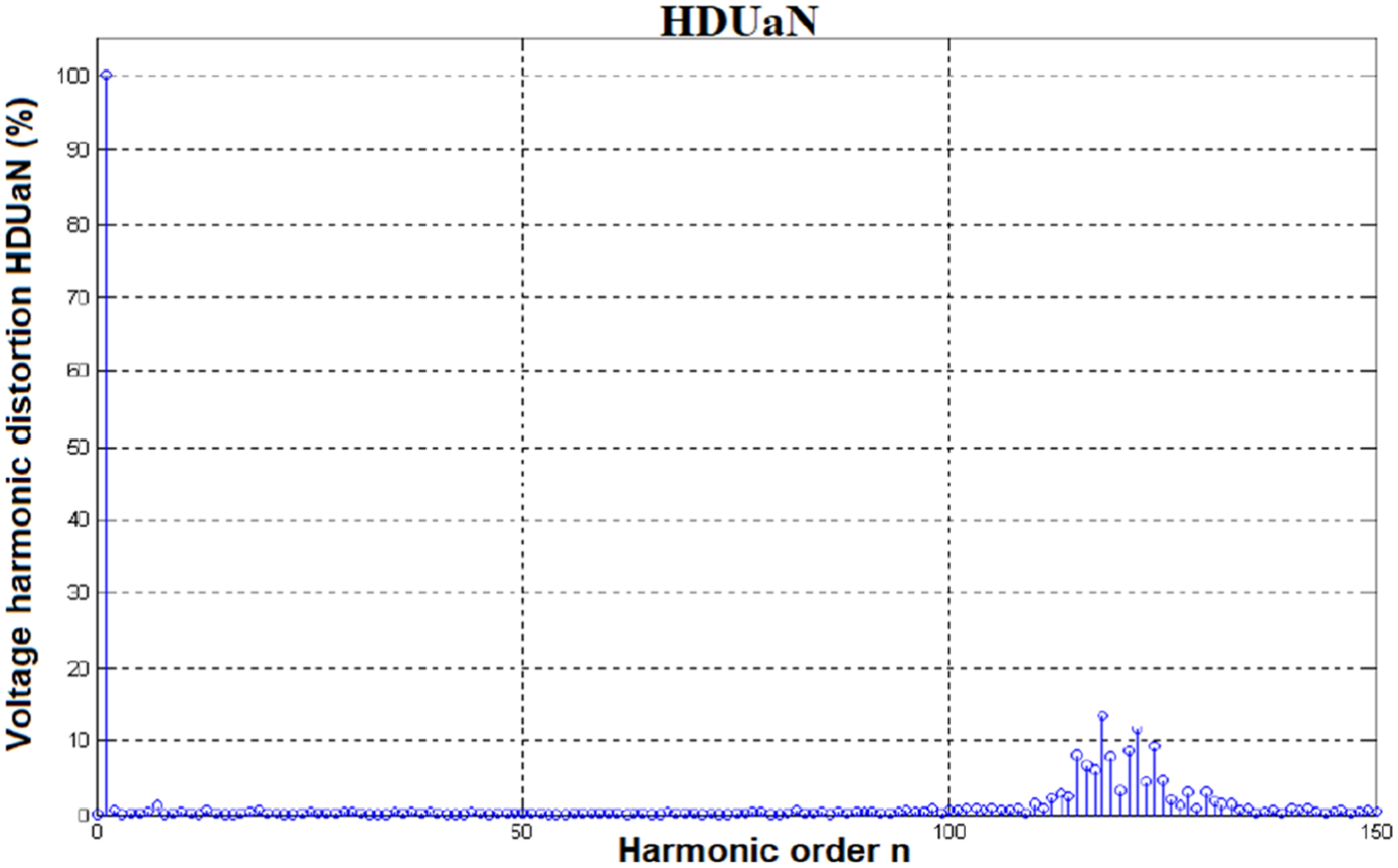
Harmonic distortion of grid voltage HDUaN (%).

Conclusion

An asynchronous wind turbine generator with full load dual AC-DC-AC power converter has not been widely used mainly because this configuration has not shown good performance in low wind speed. In this paper the principle of maximizing adopted wind power from the generator with full load dual AC-DC-AC power converter through turbine speed control, which uses the calculated maximum power of the turbine as the reference, is proposed. It is demonstrated that the drive behaves according to the predicted dynamics and thus fulfils the set goals of regulation.

The main advantage of the proposed configuration and control concept is the possibility of running the induction generator and therefore the turbine at a variable speed which allows the maximum wind power to be captured in the wide wind speed range. Furthermore, it is possible to regulate the system enabling the grid is released from the transfer of reactive power required to excite the machine. If necessary, the reactive power is injected into the grid, therefore the configuration can act as a reactive power compensator. As a result of generator speed control, the overall grid performance including voltage profile and active and reactive power losses can be significantly improved (Ciric et al., 2004).

The disadvantage of proposed regulation concept is reflected in the AC-DC-AC conversion losses, which are not negligible at the higher power conversion since the total power generated is converted twice. The rated voltage of the applied machine in simulation is 6 kV which is achievable with a two-level converter, but since the maximum voltage rating of IGBT is 6.5 kV, there is a little margin. In addition, there is a problem of generating higher current harmonics, therefore additional investment in filtering devices is needed. The future work is focused on developing of new full load power converters and strategies for control of wind turbine induction generators to maximize absorbed wind power with improved power transfer performance.

Footnotes

Appendix

Asynchronous generator parameters: P_n = 2000 kW; U_n = 6000 V; p = 4; f_n = 50 Hz; I_n = 220.3 A.

Connection: Y; cos φ = 0.9162; s_n = 0.8172; η_n = 0.9534; J = 430 kg/m²; R_s = 0.12094 Ω; R_r = 0.140784 Ω; X_ls = 1.33774 Ω; X_lr = 0.98214 Ω; X_m = 54.58 Ω.

Wind turbine and gearbox parameters: R_tur = 38.568 m; V_{wind_n}=11.47 m/second; ω_{tur_n} = 2.587 rad/second; J_tur = 1,000,000 kgm²; K_red = 30.61.

Grid parameters: U_mr = 3000 V; R_mr = 1 Ω; L_mr = 0.001 H.

DC bus parameters: C = 1000 µF; U_{dc_ref} = 10,000 V.

Generator speed controller: K_p = 0.00005; K_i = 0.03.

Generator torque regulator: K_p = 0.01; K_i = 0.4.

Generator flux regulator: K_p = 0.01; K_i = 0.1.

DC bus voltage regulator: K_p = 1; K_i = 100.

Active power regulator of the grid: K_p = 0.01; K_i = 2.

Reactive power regulator of the grid: K_p = 0.01; K_i = 2.

Declaration of conflicting interests

The author(s) declared no potential conflicts of interest with respect to the research, authorship, and/or publication of this article.

Funding

The author(s) received no financial support for the research, authorship, and/or publication of this article.

ORCID iD

Rade M Ciric

References

Abuaisha

(2014) General study of the control principles and dynamic fault behaviour of variable-speed wind turbine and wind farm generic models. Renewable Energy 68: 245–254.

Analog Devices (2000) Implementing SVM with the ADMC 401.http://www.analog.com/en/products/admc401.html (accessed 23 November)

Araghi

Riahy

Carlson

, et al. (2020) Enhancing the net energy of wind turbine using wind prediction and economic NMPC with high-accuracy nonlinear WT models. Renewable Energy 151: 750–763.

Bechir

Faouzi

Gasmi

(2012) Wind energy conversion system with full-scale power converter and squirrel cage induction generator. International Journal of the Physical Sciences 7(46): 6093–6104.

Behnkel

Muljadi

(2005) Reduced order dynamic model for variable-speed wind turbine with synchronous generator and full power conversion topology. In: Proceedings of the future power systems international conference, 18 November 2005, Amsterdam, Netherlands, pp.1–6.

Cardenas

Pena

(2004) Sensorless vector control of induction machines for variable-speed wind energy applications. IEEE Transactions on Energy Conversion 19: 196–205.

Ciric

Padilha-Feltrin

Denis

IFED

(2004) Observing the performance of distribution systems with embedded generators. European Transactions on Electrical Power 14: 347–359.

Deshpande

Kalange

Lokhande

(2018) Output power maximization of wind energy conversion system using doubly fed induction generator. In: 8th IEEE India international conference on power electronics, 13–15 December 2018, Jaipur, India.

Divya

Rao

PSN

(2006) Models for wind turbine generating systems and their application in load flow studies. Electric Power Systems Research 76: 844–856.

10.

Ekanayake

Holdsworth

Jenkins

(2003) Dynamic modeling of doubly fed induction generator wind turbines. IEEE Transactions on Power Systems 18: 803–809.

11.

Gitano-Briggs

(2010) Small Wind Turbine Power Controllers. Penang, Malaysia: University Science Malaysia.

12.

Hiti

Borojevic

(1994) Control of front-end three–phase boost rectifier. In: Proceedings of the applied power electronics conference, Orlando, FL.

13.

Inthamoussou

De Battista

Mantz

(2016) LPV-based active power control of wind turbines covering the complete wind speed range. Renewable Energy 99: 996–1007.

14.

Jiao

Ooi

Joós

, et al. (2005) Doubly-fed induction generator (DFIG) as a hybrid of asynchronous and synchronous machines. Electric Power Systems Research 76: 33–37.

15.

Ledesma

Usaola

(2005) Doubly fed induction generator model for transient stability analysis. IEEE Transactions on Energy Conversion 20: 388–397.

16.

Mansouri

Mimouni

Benghanem

, et al. (2004) Simulation model for wind turbine with asynchronous generator interconnected to the electric network. Renewable Energy 29: 421–431.

17.

Marcetic

(2014) Microprocessor Control of Power Converters. Novi Sad: University of Novi Sad, Faculty of Technical Science.

18.

Martins

Perdana

Ledesma

, et al. (2007) Validation of fixed speed wind turbine dynamic models with measured data. Renewable Energy 32: 1301–1316.

19.

Maxime

(2000) Review of electromechanical conversion in wind turbines. TU Delft. DOI:10.13140/RG.2.2.25876.30087, Report number: EPP00.R03

20.

Mei

Jiang

(2012) Research on squirrel-cage induction generator full power converter control strategies of wind power generation system with dynamic systems. Advanced Materials Research 496: 104–108.

21.

Mérida

Aguilar

Dávila

(2014) Analysis and synthesis of sliding mode control for large scale variable speed wind turbine for power optimization. Renewable Energy 71: 715–728.

22.

Mihet-Popa

Blaabjerg

Boldea

(2004) Wind turbine generator modeling and simulation where rotational speed is the controlled variable. IEEE Transactions on Industry Applications 40: 3–10.

23.

Pesic

(1994) Wind Energy, Aerodynamics of Wind Energy Systems With Horizontal Rotation Axis. Belgrade: Faculty of Mechanical Engineering.

24.

Pesut

Ciric

(2020) Speed control of grid connected asynchronous wind turbine generator by dual AC-DC-AC converter. In: Proceedings of 2020 mediterranean conference of power generation, transmission, distribution and energy conversion, MedPower2020, Cyprus, 9–12 November 2020.

25.

Rawn

Lehn

Maggiore

(2006) Toward controlled wind farm output: Adjustable power filtering. In: IEEE power engineering society general meeting, 18–22 June 2006, Montreal, QC, Canada.

26.

Singh

Sundaram

Matuonto

(2021) A solution to reduce overheating and increase wind turbine systems availability. Wind Engineering 45: 491–504.

27.

Slootweg

de Haan

Polinder

, et al. (2003) General model for representing variable speed wind turbines in power system dynamics simulations. IEEE Transactions on Power Systems 18: 144–151.

28.

Tapia

Ostolaza

, et al. (2003) Modeling and control of a wind turbine driven doubly fed induction generator. IEEE Transactions on Energy Conversion 18: 194–204.

29.

Tapia

Ostolaza

(2006) Two alternative modeling approaches for the evaluation of wind farm active and reactive power performances. IEEE Transactions on Energy Conversion 21: 909–920.

30.

Trudnowski

Gentile

Khan

, et al. (2004) Fixed-speed wind-generator and wind-park modeling for transient stability studies. IEEE Transactions on Power Systems 19: 1911–1917.

31.

Vukosavic

(2010) Electric Machines. Belgrade: Academic Mind.

32.

Yin

Lin

, et al. (2016) Hydro-viscous transmission based maximum power extraction control for continuously variable speed wind turbine with enhanced efficiency. Renewable Energy 87: 646–655.

An efficient method for speed control of induction wind turbine generator with dual AC-DC-AC converter

Abstract

Keywords

Introduction

Model of energy converter

Generator control

DC-bus voltage control

Vector control of power flow

Simulation results

Simulations on average model of PWM converter

Simulations on switching model of PWM converter

Power quality issues

Conclusion

Footnotes

Appendix

Declaration of conflicting interests

Funding

ORCID iD

References