
Abstract
High-speed electrical machines (HSEMs) are becoming more popular in applications such as air handling devices. Using surface-mounted permanent magnet (PM) rotors manufactured from rare earth metals, they provide benefits over their mechanical transmission counterparts. However, these PMs have low tensile strength and are prone to failure under large centrifugal loads when rotating. Therefore, retaining sleeves are used to hold the PMs in compression to eliminate tensile stress and reduce failure risk. The magnets are also often held on a back iron or carrier, forming an assembly of three cylinders. The ability to predict these stresses is extremely important to rotor design. Current published work shows a lack of exploration of analytical methods of calculating these stresses for three-cylinder assemblies. This paper shows the development of plane stress, plane strain and generalised plane strain (GPS) theories for three cylinders. For a range of rotor designs, these theories are compared with finite element analysis (FEA). GPS is shown to be more accurate than plane stress or plane strain for the central region of long cylinders. For short cylinders and for the ends of cylinders, all three theories give poor results.
Keywords
Introduction
HSEM usage has increased over the last 10 years due to the performance benefits over their mechanical counterparts. 1 Current literature discuss how HSEMs provide benefits in reliability and power density1–3 while the reduced weight and size of HSEMs is also beneficial.4,5 HSEMs rotate via electromagnetic forces which gives an improvement in reliability over rotors using parts in contact.6,7 Sintered PMs such as Samarium Cobalt or Neodymium are used which provide high energy density to allow the reduction of rotor size, 8 which leads to an increase in operating speed. 9
‘Interior’ (IPM) and ‘surface-mounted’ (SPM) PM rotors are the two possible rotor configurations. IPM rotors have PMs buried within the shaft or rotor iron while SPM rotors have PMs bonded to the surface of the shaft or rotor iron. 8 Due to the sintering process, the Samarium Cobalt and Neodymium magnets have low tensile strength. When the magnets are mounted to a shaft or carrier cylinder, a sleeve is required to keep them in compression to avoid tensile stresses. These stresses are critical to the rotor durability so they must be calculated accurately.8,10 SPM rotors are recommended for high-speed operation despite often being constructed using three or more interfering cylinders. This is due to the stress concentrations generated within IPM rotors limiting operating speed. Whilst the sleeve in SPM rotors reduces efficiency, as it acts as an electromagnetic air gap, this is not as limiting as IPM stress concentrations.10,11 Therefore, a reliable theoretical method of calculating stresses in a three-cylinder rotor during operation is required.
The current work done on this topic has shown a lack of investigation into theoretical analyses for three-cylinder rotors. 12 Accurate theoretical analysis enables the validation of FEA simulations and also provides a more efficient method of predicting rotor stresses than running FEA studies for multiple topologies. For the papers that have completed theoretical analysis, the majority use plane stress13–15 or plane strain9,16,17 theory methods.
For the plane stress analyses, Zhu and Chen 14 state their model is not bound by an axial load, while Cheng et al. 15 states their rotor is under a small axial load and therefore, both assume plane stress condition. Zhang et al. 13 found little difference between the plane stress and plane strain approaches for their model and chose plane stress due to simplicity. All of these papers13–15 discuss three-cylinder rotors, but all simplify the analytical model to calculate the stresses for two-cylinders.
For the plane strain theory approach, three-cylinder rotors are also discussed.9,16 Burnand et al. 9 provides equations for all three cylinders, however it is assumed that there is no interference present between the shaft and the magnets, leaving a two-cylinder approach with one interference location. Zhou and Fang 16 also focus on three-cylinder rotors, but similarly the analysis equations only relate to two interfering cylinders. Papini et al. 17 makes no discussion of any interfering surfaces within their models.
There has been a lack of investigation into alternative theoretical approaches, but none have developed a theoretical model taking three cylinders, with two interference locations, into account. The final recommendation, from Mallin and Barrans, 12 for the theoretical analysis was to use the GPS approach instead of plane strain or plane stress. This paper will develop the plane stress, plane strain and GPS theories for three-cylinder rotors, examine the differences between each theory for the same rotor design and will benchmark these results against FEA simulations.
Classical closed-form analysis techniques
Background
The analysis described here will be applicable to rotors constructed using three interfering cylinders, with the magnets being mounted on an inner carrier or back iron. It is assumed that this carrier does not interfere with the central shaft. Figure 1 shows how the rotor would be configured on a shaft in a HSEM.
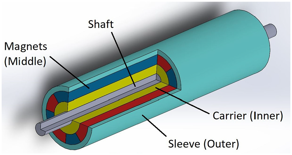
Three cylinder rotor set-up on a HSEM shaft.
Figure 2 shows the configuration and corresponding location nomenclature. While each pair of interfering cylinders meets at a common radius, the initial radial dimensions, before assembly, are shown via the horizontal dashed lines. The overlap of cylinder diameters creates the necessary interference to keep the rotor together at all times. Therefore,
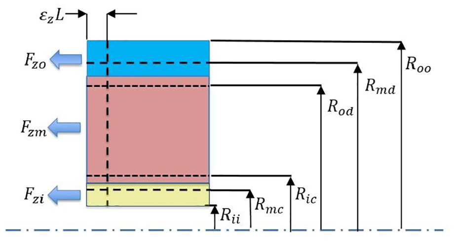
Three cylinder axial cross-section.
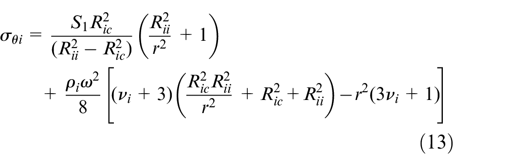
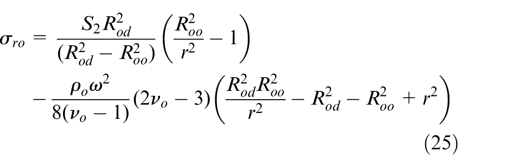
For such three-cylinder rotor configurations: no radial stress is applied to
From this, a set of boundary conditions are derived for each cylinder, where r is the variable radial dimension and
For the inner cylinder:


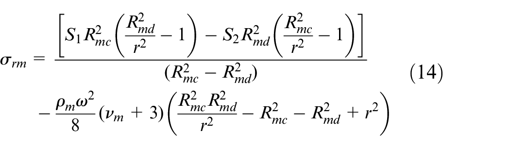
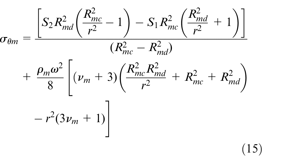
For the magnet cylinder:


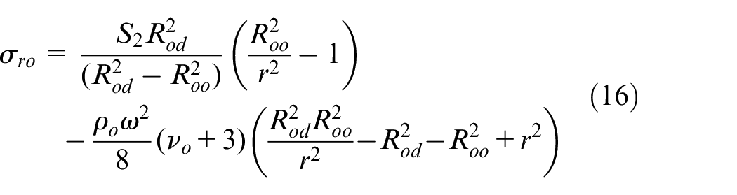
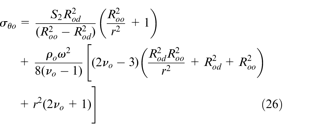
For the outer cylinder:


The boundary conditions are then applied to the corresponding equations for each theoretical approach. The following assumptions are made for the theoretical analyses:
No load is applied to the rotor in the axial direction.
The radial and circumferential stresses are uniform along the length of the rotor.
No interactions with the surroundings for the inner and outer surfaces of the rotor.
The friction between the interfering cylinder surfaces is high enough to prevent slip.
Due to the cylinder interference, compatibility conditions must also be placed on the analyses. These compatibility conditions are:
At the inner common radius:

At the outer common radius:

Where
As shown by Mallin and Barrans, 12 SPM rotor designs often use segmented PMs. The theoretical approaches presented here assume the PM cylinder is a solid body and cannot predict the interactions between each magnet. Therefore, rotor designs with interpole gaps will not be suitable for the calculations. In these rotors, as shown by Chen et al. 18 the stress in the sleeve spikes at the edges of the magnets. To accommodate this high stress, the sleeve has to be strengthened. However, designs without interpole gaps will be suitable for analysis using approaches presented here, despite using segmented magnets. As discussed by Barrans et al., 8 the magnets must always be held in compression; therefore, the PMs are always in contact and can be assumed to act as a solid body.
Plane stress
Plane stress is the simplest and most common theoretical approach to thick-walled cylinder stress approximation. It is a suitable approximation method for cylinders which are short relative to their diameter (i.e. disks). In a thin disk the resistance to change in thickness (the axial dimension) is insignificant. Hence, axial stress,
The radial (
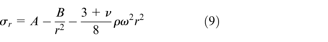
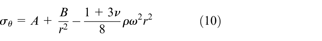

Where
Boundary conditions (1) to (6) are substituted in to (9) for each cylinder to eliminate constants A and B. For each cylinder, equations (9) and (10) can then be rewritten in terms of the shrinkage pressures,

With the stress equations developed, the circumferential strains,
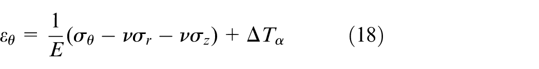
Substituting the circumferential strain equations obtained into the compatibility conditions expressed in equations (7) and (8) allows
Plane strain
Whereas plane stress assumes that there is no restriction to axial deformation, the plane strain assumption is that axial deformation is completely restrained. This modelling approach is used less frequently as discussed in Mallin and Barrans. 12 This method is more complex than plane stress as axial stress will not be zero. However, the assumption that axial strain is zero enables a simplified equation for axial stress.
As shown by Barrans et al., 8 plane strain follows the same method as plane stress but starts with the following equations for circumferential and radial stress, instead of equations (9) and (10).
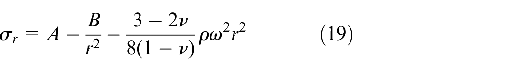
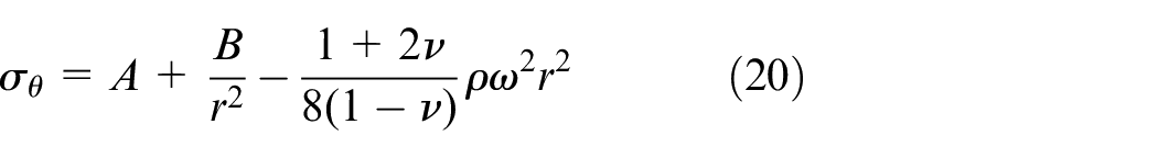
Constants A and B are found by introducing the boundary conditions (1) to (6) depending on the cylinder of interest. The radial and circumferential stresses at key points within the compound cylinder are then given by:
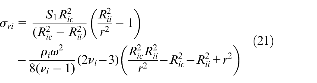
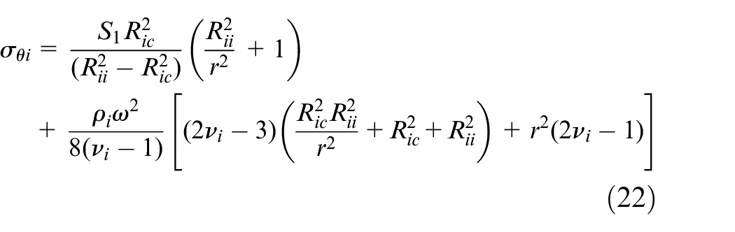
To be able to apply the compatibility conditions, the circumferential strain equations must be derived, as in the plane stress case. The circumferential and radial stress equations for each of the four cylinder surfaces at radii

The radial and circumferential stress equations for a specific surface are then substituted into equation (27) to derive the full axial stress equation. This is then used in (18) along with the circumferential and radial stress equations, to derive the full circumferential strain equation. This is completed for all four cylinder surfaces of interest where the example below, equation (28), shows the circumferential strain at
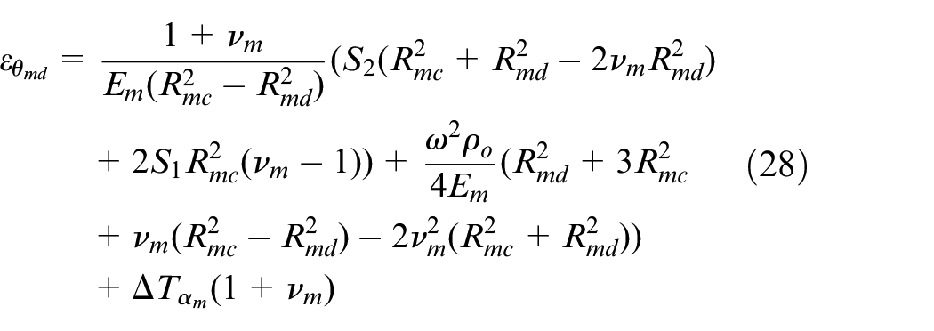
The circumferential strain equations are then substituted into (7) and (8), to enforce the compatibility conditions and can be used to solve for
New theory: Generalised plane strain
Applying the GPS model to rotating thick walled cylinders, it is assumed that the axial strain does not vary with respect to radial or circumferential position. The application to an assembly of three cylinders presented here follows previous work in Barrans et al. 8 for two interfering cylinders. It is assumed that there is a high enough level of friction between the cylinders to avoid slip. Similarly to the plane strain method, axial stress is not assumed to be zero. However, instead of assuming axial strain to be zero, GPS assumes axial strain is also present, but is constant through the wall of the cylinder. In the interest of brevity, an example derivation for the middle cylinder is shown below. The inner and outer cylinders follow a similar method.
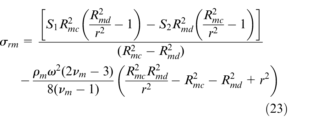
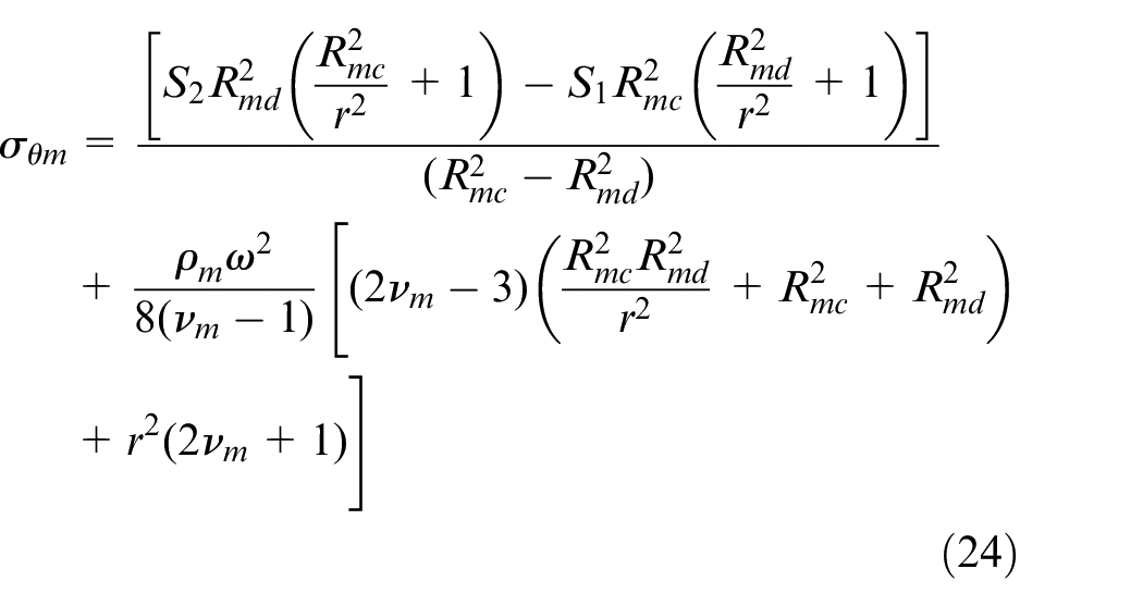
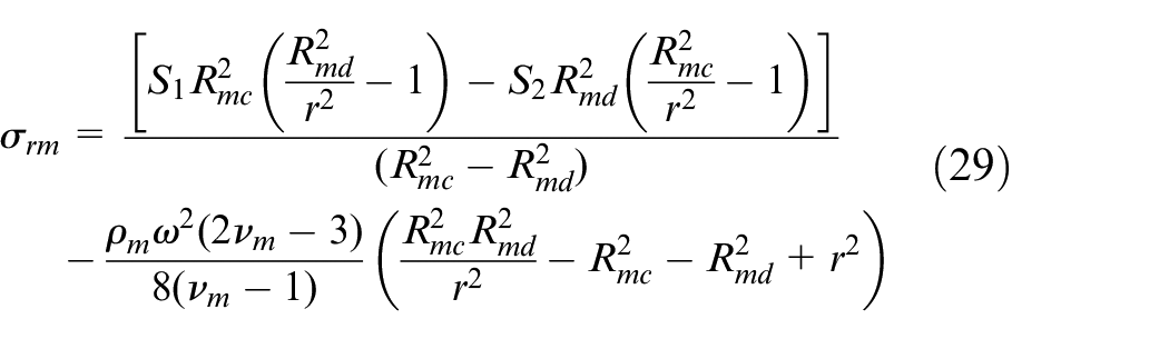
GPS starts with the same initial equations as plane strain, equations (19) and (20), solving for A and B using the boundary conditions (3, 4). A and B are then substituted back into (19) and (20) to give the full radial and circumferential stress equations:

To determine the axial stress the condition of constant axial strain is combined with equations (19) and (20) within Hooke’s law to give:
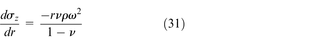
Hence:
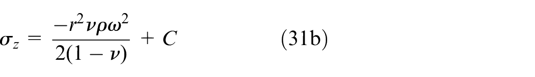
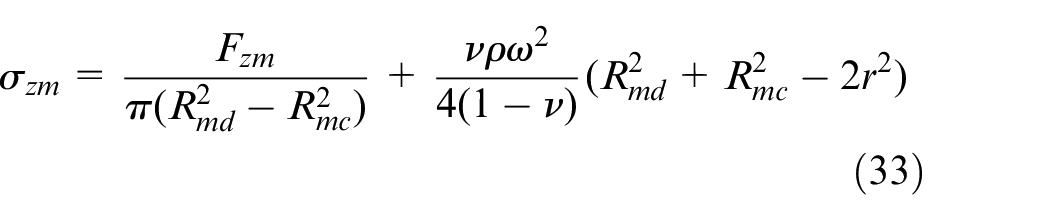
Where C is a constant. The axial force,
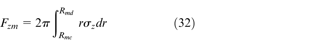
Using this, the constant C in equation (31b) can be determined and that equation can then be written as:
The GPS method has additional unknown values that must be solved to calculate cylinder stresses. These are the axial forces acting on each of the interfering cylinders. Therefore, GPS is subject to more compatibility conditions than plane stress or plain strain. These are:
There must be radial force equilibrium between the interfering cylinder surfaces. This is represented with
There must be circumferential compatibility between the interfering cylinders because in practice, the cylinder surfaces come together at a common radius. Represented by equations (7) and (8).
There must be axial strain compatibility due to the assumption of enough friction to avoid slip.


Where
There must be equilibrium between the axial forces within the three cylinders. This can be given by:


Where
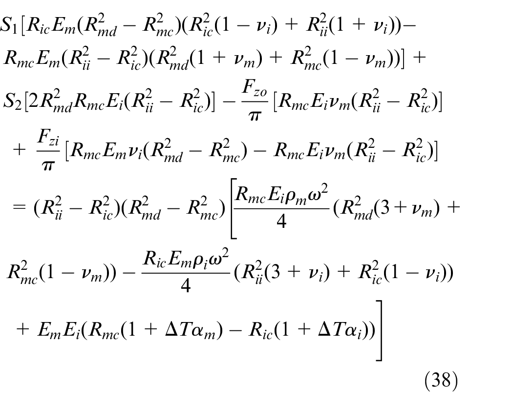
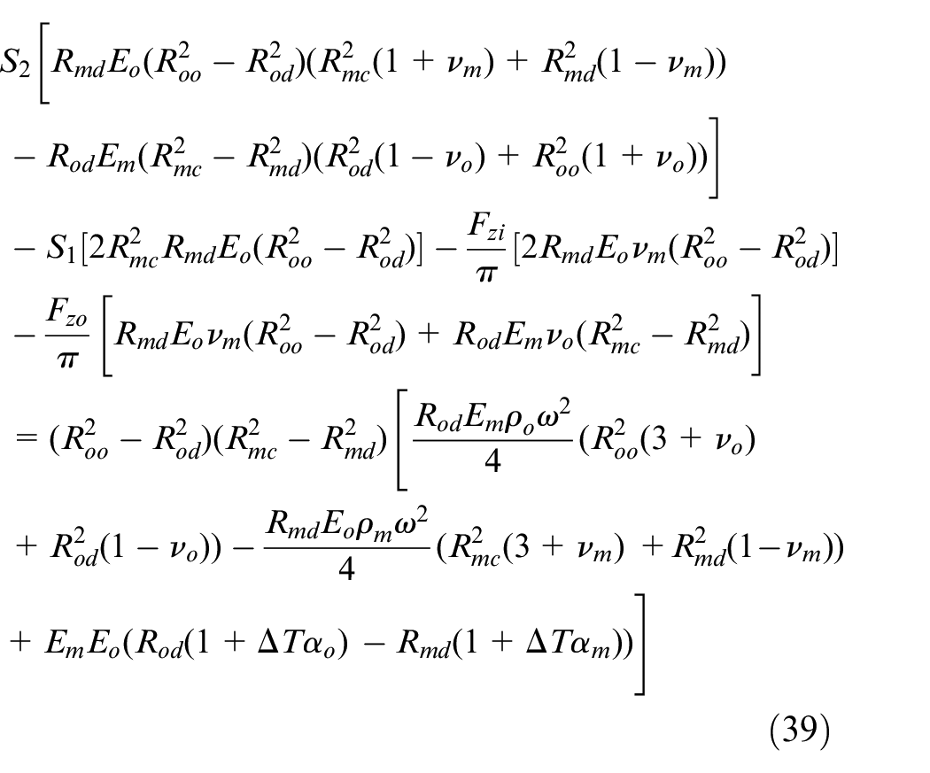
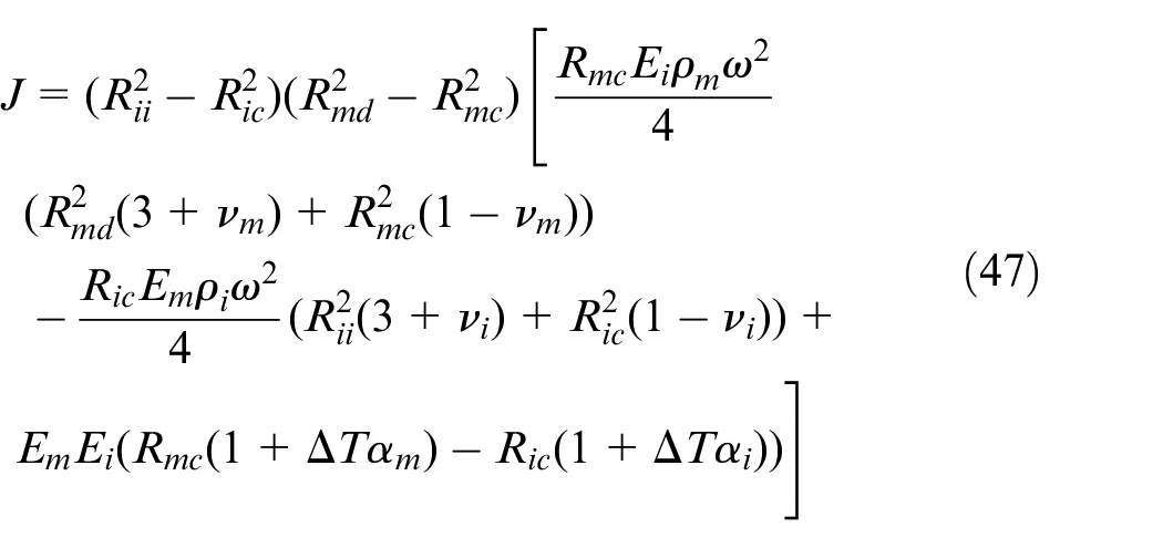
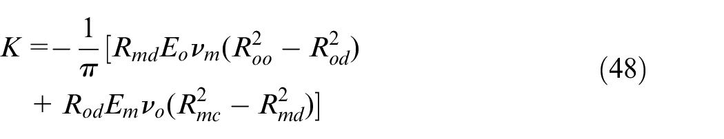
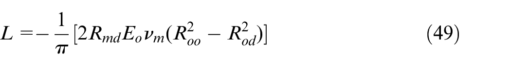
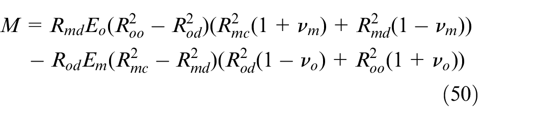
Equations (29), (30) and (33) (and their equivalents for the inner and outer cylinders) and equation (18) can be used to determine the circumferential strains at each interfering surface. These can be combined with equation (37) and then substituted in equations (7) and (8) to enforce conditions B and D, giving:
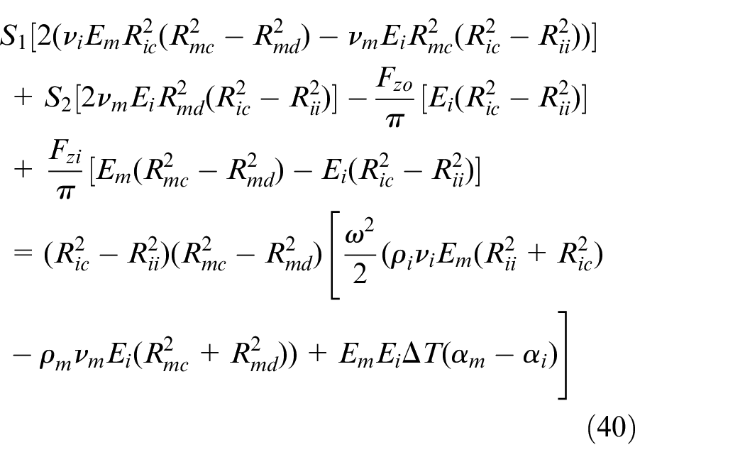
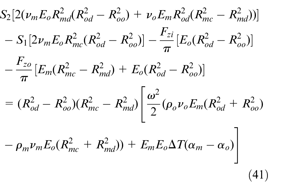
To enforce condition C, axial strain equations for each cylinder are derived using Hooke’s law and are then substituted into (34) and (35) to give:
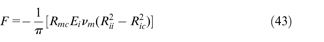
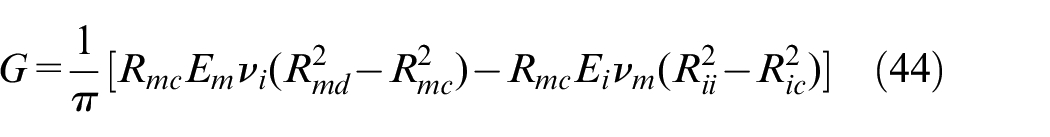
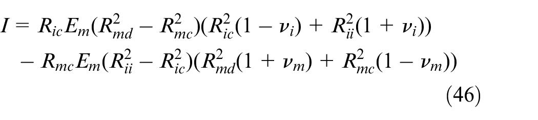
The axial force for the magnet cylinder,
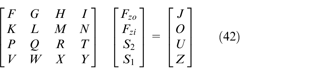
Where:


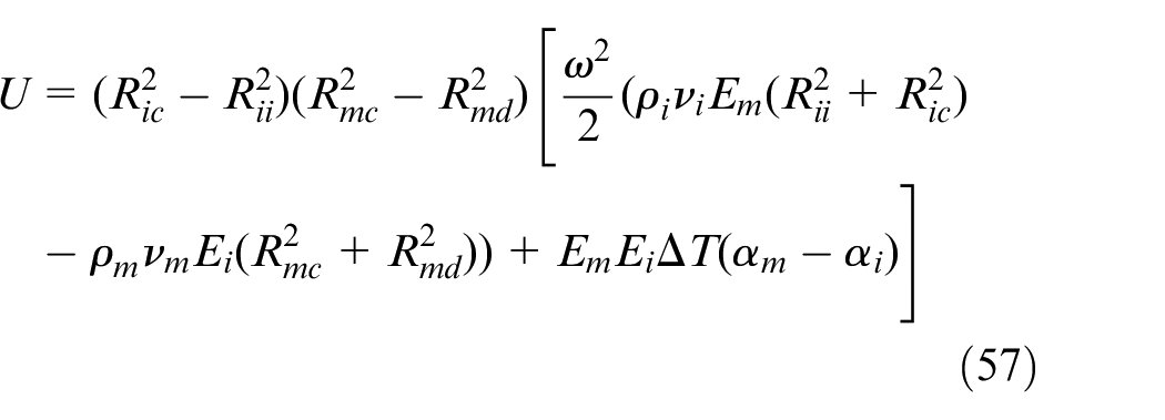
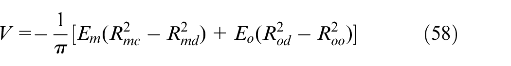
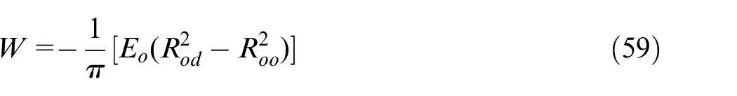
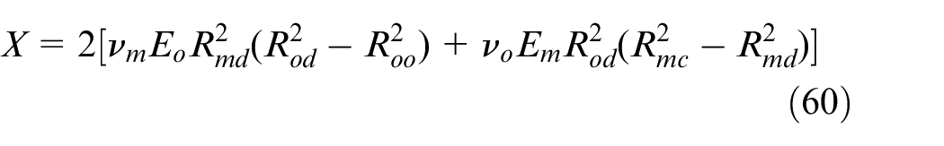

The unknown terms can then be found by inverting the matrix. Having determined these terms, stresses at any location can be found by referring back to equations (29), (30) and (33) and their equivalents for the inner and outer cylinders.
All rotors were simulated at four conditions:
Stationary and ambient temperature.
Maximum speed and ambient temperature.
Stationary at maximum temperature.
Maximum speed and temperature.
Finite element analysis
To investigate possible limitations of the theoretical approaches, a range of finite element analyses were carried out on rotors with the material properties and dimensions shown in Tables 1 and 2 respectively. These geometries were selected recognizing that, as demonstrated by Barrans et al.,
8
the length to diameter ratio of the rotor can have a significant effect on the stress distribution. The rotors were defined as running at
Material properties for each cylinder.
Model rotor parameters.
Based on the review by Mallin and Barrans, 12 an axisymmetric model was selected for the analysis. A 2D radial section analysis would not have been suitable as the change in stresses along the axis could not have been simulated to explore the ‘end-effect’. A full 3D FEA model would have yielded no further information regarding the stress and strain distribution and would therefore have been inefficient. Recognising the axial symmetry present, only half of the rotor length was modelled and an axial displacement constraint applied. Figure 3 shows one of the FEA models with three cylinders and the axial symmetry and displacement conditions in place. The dashed line represents the rotor axis.
FEA model.
Once the rotor was created, the simulation conditions were specified. An interference fit with ‘small sliding’ condition was applied to interfaces c and d. The ‘small sliding’ formulation assumes that there is no significant tangential motion between the two surfaces and is appropriate in this case. During the first analysis step, the interfering surfaces were moved to a common radius. Since the surfaces cannot intersect, ‘hard’ contact was specified between the surfaces. In the tangential direction, a coefficient of friction of 1 was specified. Separation of the surfaces was allowed as this enabled the FEA to predict when the centrifugal force from rotation would become too large for the rotor to withstand.
Figures 4 and 5 show the axial stress results for the long and short thin-rotor simulations respectively at
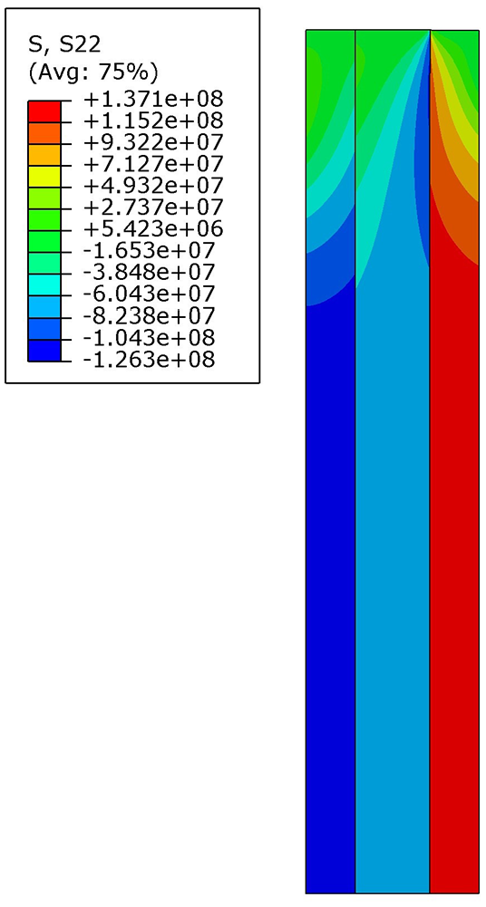
Thin long rotor axial stress results.
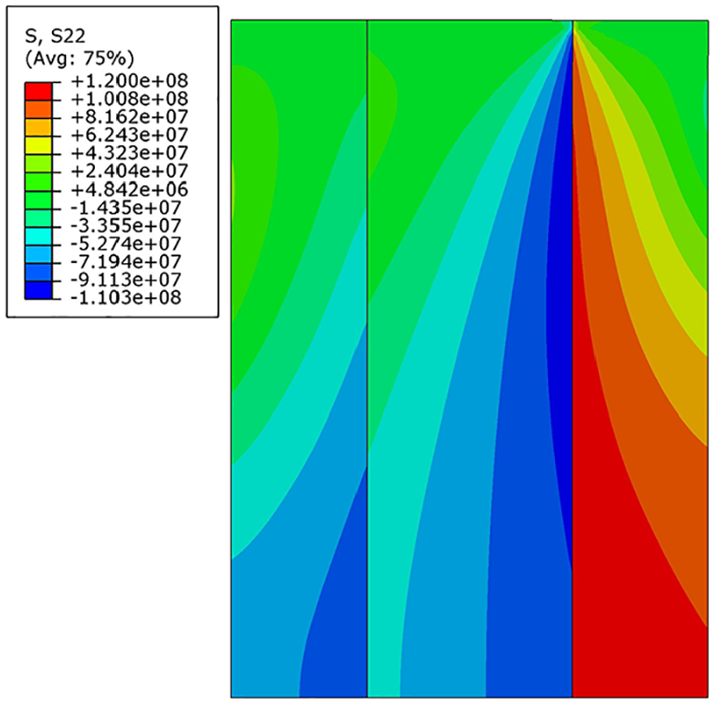
Thin short rotor axial stress results.
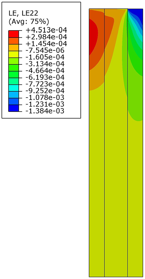
Thin long rotor axial strain results.
Theoretical analysis results
An example of the results gathered from the FEA simulations is shown in Table 3. The probed stress components were: contact pressures at c and d (
FEA probed result example.
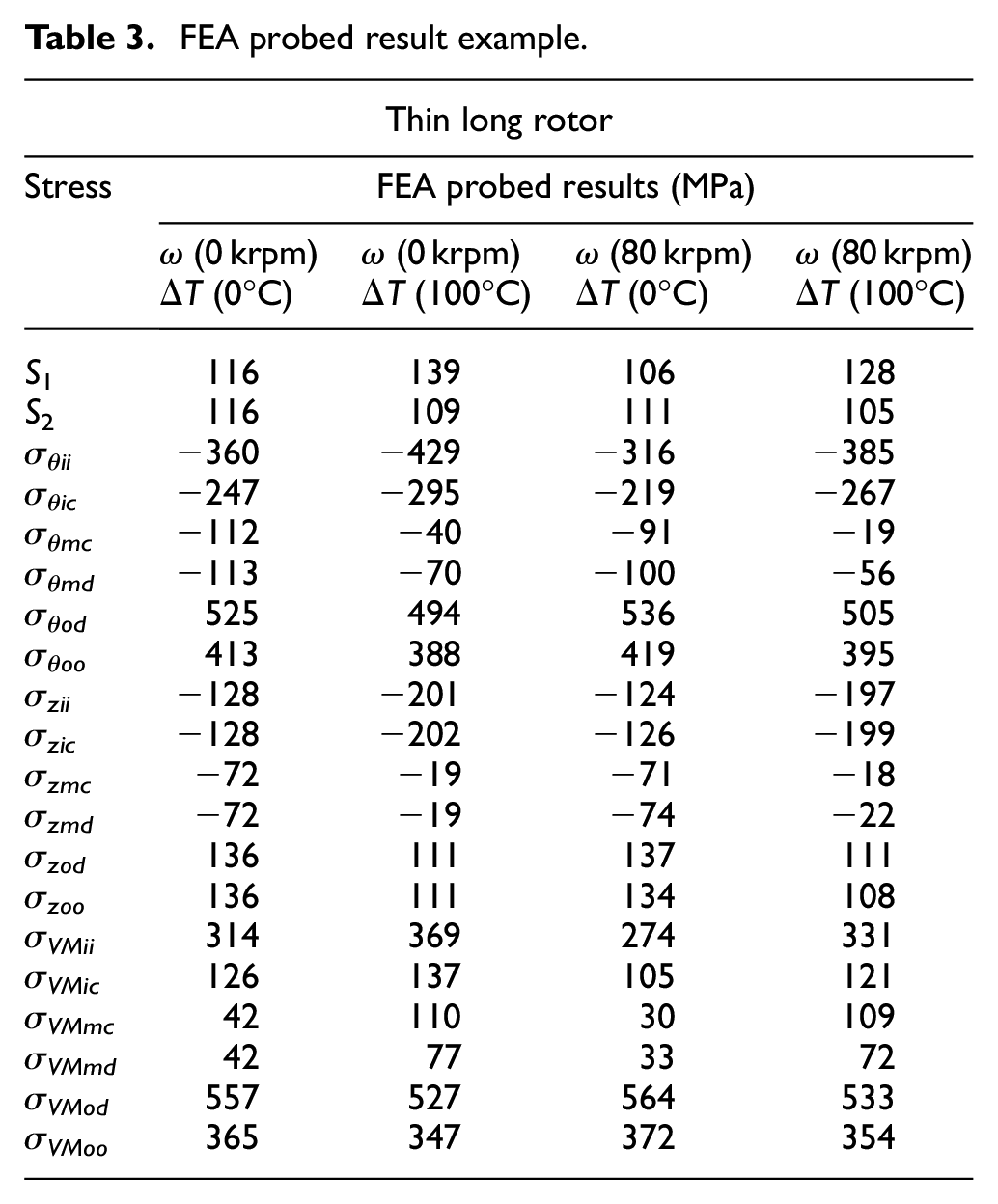
These stresses were selected because:
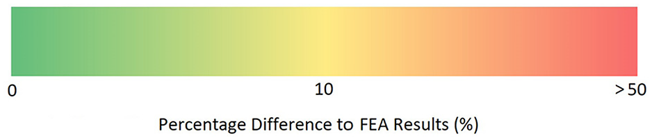
The FEA results presented in this section were compared against the results from each theoretical analysis. Results were probed from the plane of axial symmetry, where end effects not accounted for in the theoretical approaches will be minimal. A percentage difference to the FEA was calculated for each result, to enable easy comparison across analyses. Percentage difference results were also colour coded to highlight which results were close to the FEA using the scale shown in Figure 7.
Long rotor results
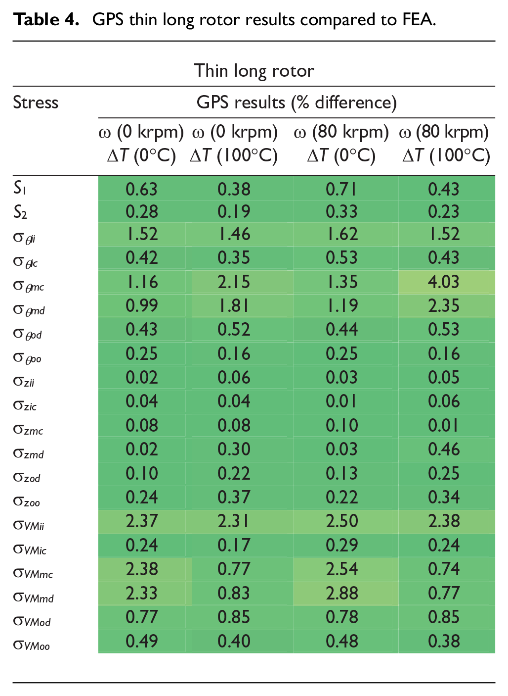
Table 4 shows the GPS results for the thin long rotor. To present the results graphically, a histogram was plotted to display the frequency that a result occurred, shown in Figure 8. The range of results were split into bins and the number of results falling into each bin was tallied, showing how the differences to the FEA results are distributed. For the thin long rotor, 76% of the GPS results are within ±1% of the FEA results, while 86% fall within ±2% of the FEA. This accuracy is similar across all operating conditions, which shows it is a robust theoretical analysis method for thin long rotors. Tables 5 and 6 show the same results for the plane strain and plane stress respectively. They are then compared in Figure 9.
GPS thin long rotor results compared to FEA.
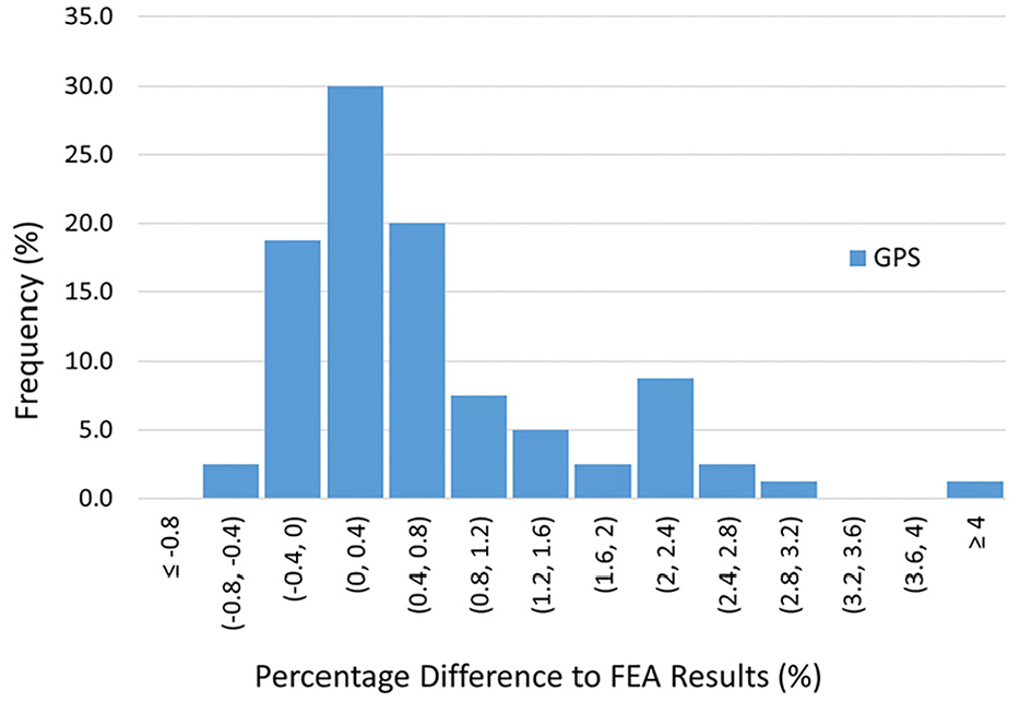
Thin rotor – GPS results histogram.
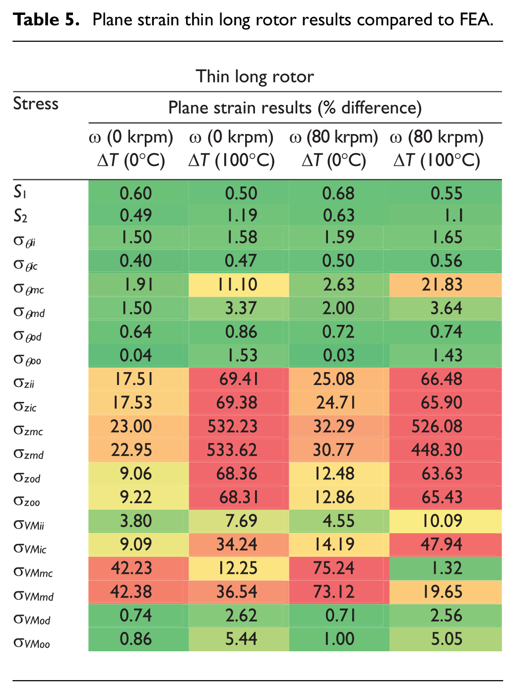
Plane strain thin long rotor results compared to FEA.
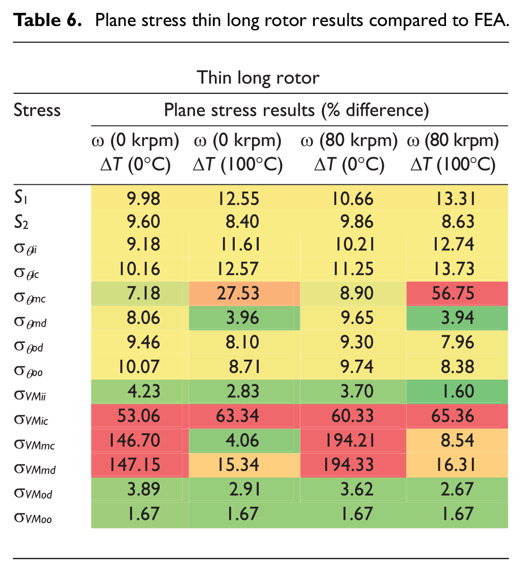
Plane stress thin long rotor results compared to FEA.
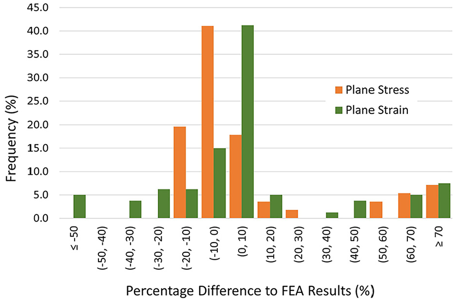
Thin rotor – plane strain and plane stress results histogram.
Table 5 shows that the plane strain theory has similarly accurate results as GPS, for the circumferential stresses, when the rotor is stationary or at speed. However, the axial stress results are much less accurate and when temperature is increased, the accuracy is severely affected further. This is due to plane strain assuming there is no axial strain in the rotor. Effectively, this places the rotor between rigid bodies, inducing compressive stress, affecting the results. The inaccuracies with the axial stress are then carried over into the Von Mises stress. Figure 9 shows both plane stress and plane strain produce much larger differences than the GPS for thin long rotors. The axial stress results were not included for plane stress as the theory assumes axial stress to be zero.
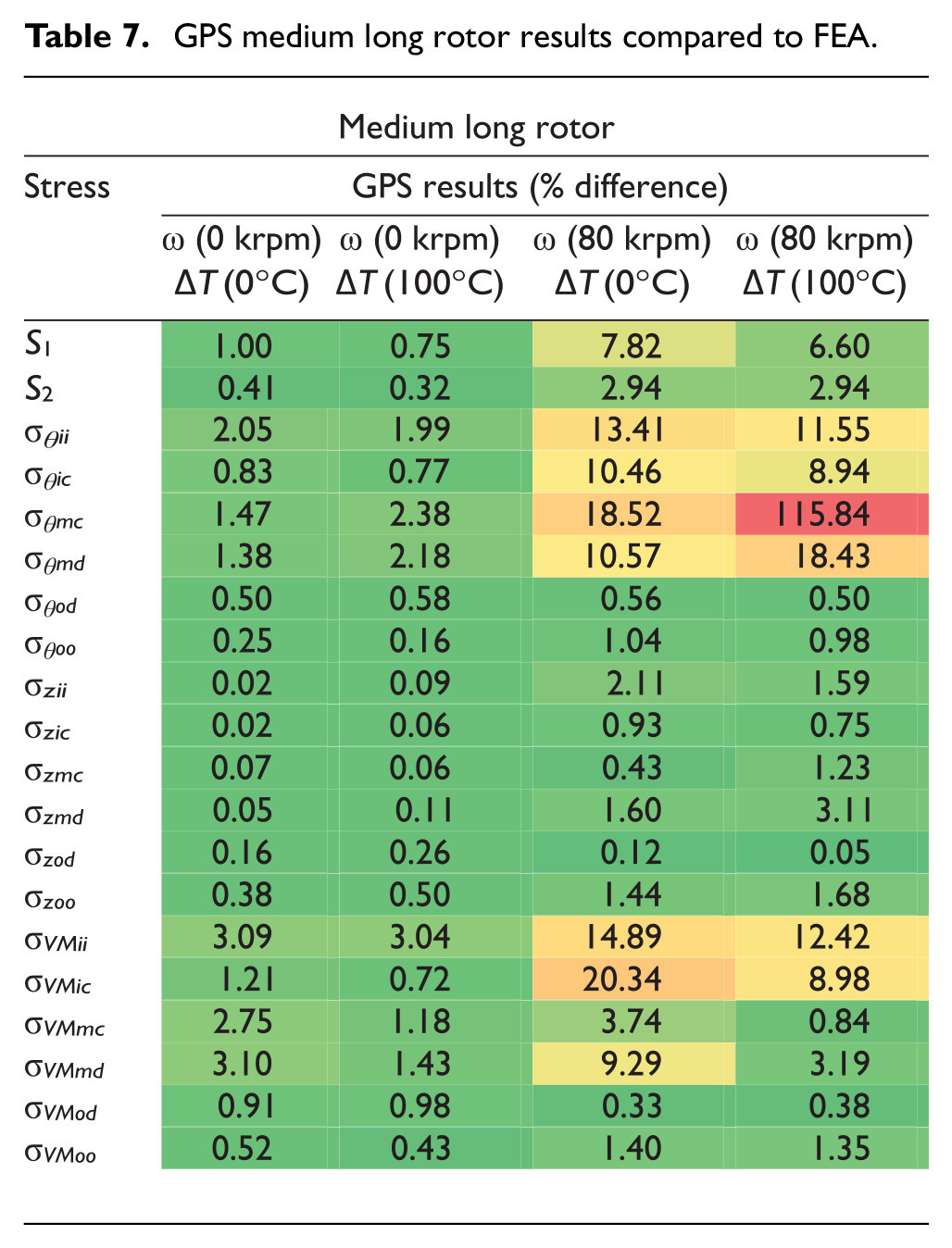
The accuracy shown in Table 4 is closely replicated with the medium and thick versions of the long rotor when stationary. The results are shown in Tables 7 and 8. It is important to note that the FEA simulation for both the medium and thick long rotors, predicted the cylinders would separate at c. This only occurred at the rotor ends and only at full operating speed with no elevated temperature. At operating speed with elevated temperature, the pressure at c at the rotor ends was also significantly reduced. This appears to have affected the accuracy of
GPS medium long rotor results compared to FEA.
GPS thick long rotor results compared to FEA.
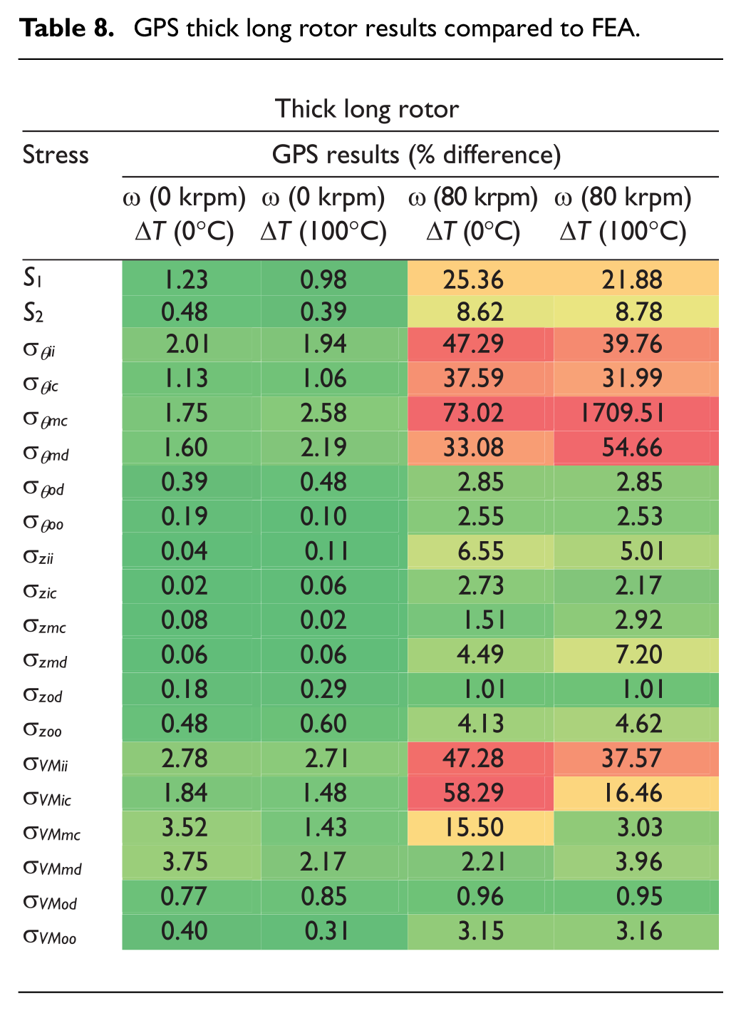
Figure 10 shows the end separation at c predicted by the FEA for the medium and thick rotors from Tables 7 and 8. The thick rotor separates more and this is shown by the larger difference in
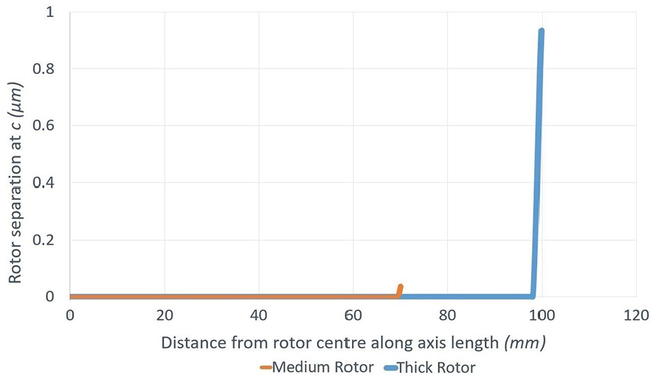
Rotor end separation at c.
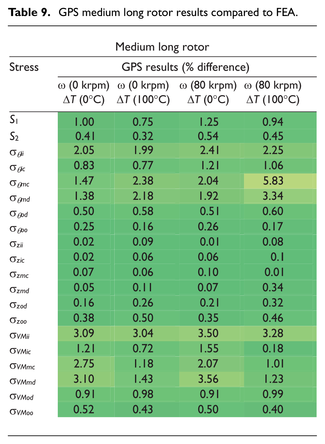
The medium and thick long rotor topologies were then run at a lower speed to avoid separation at the rotor ends and the results accuracy improved greatly. Tables 9 and 10 show the medium long rotor at
GPS medium long rotor results compared to FEA.
GPS thick long rotor results compared to FEA.
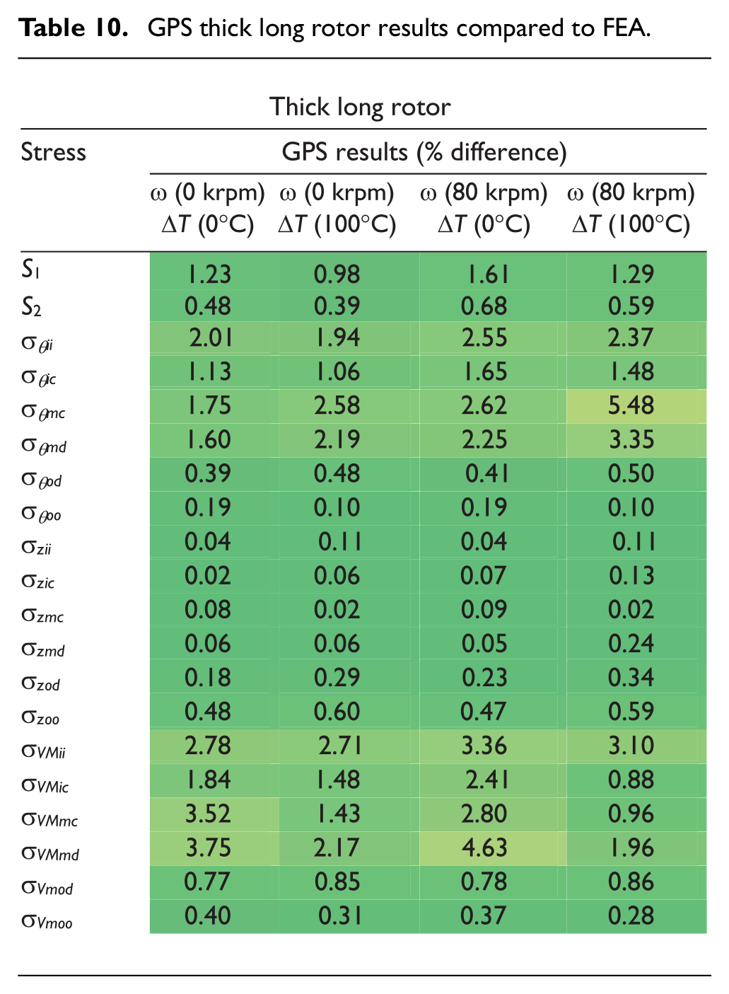
Figure 11 shows the histogram of the GPS results for each cylinder without separation at c. The thin cylinder has more results concentrated towards 0% and the accuracy then decreases slightly as the cylinder thickness increases. The average accuracy shifts further from 0% with each increase in cylinder thickness, reducing the probability of obtaining the most accurate results. However, even the thick cylinder still has 76% of results falling within a ±2% range and 91% within ±3% of the FEA results. This is far more accurate than the corresponding plane stress and plane strain results.
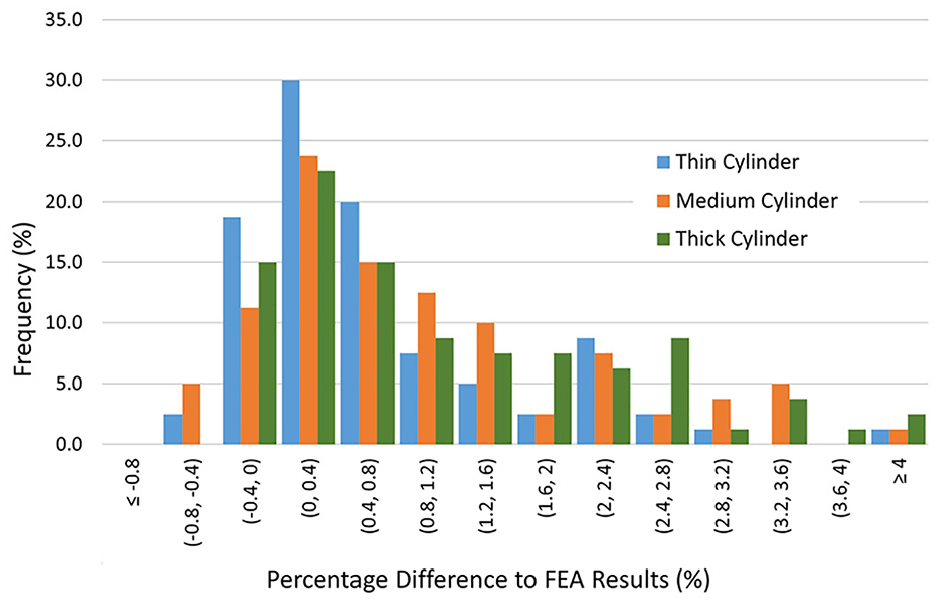
Histogram of GPS long rotor results.
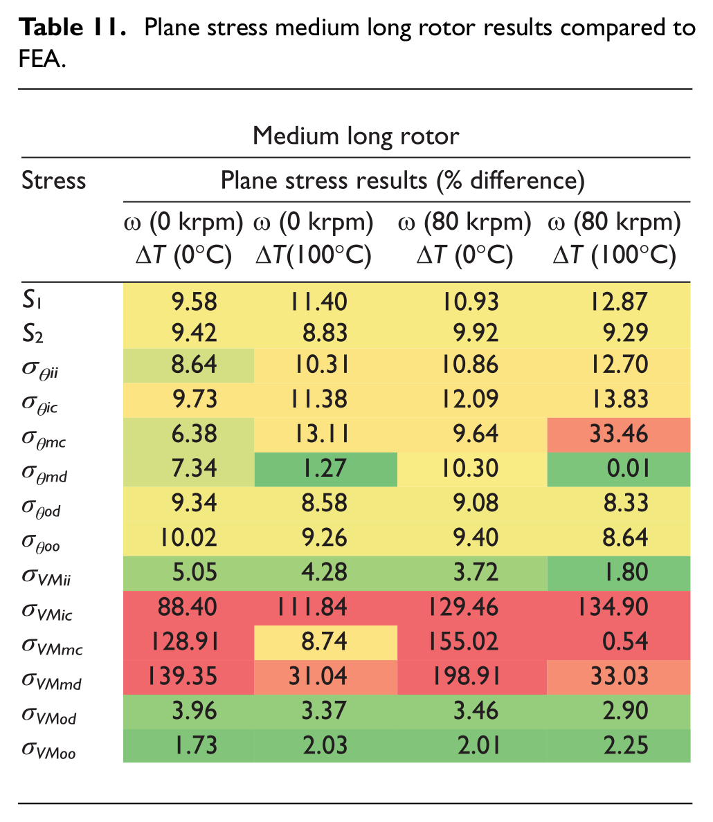
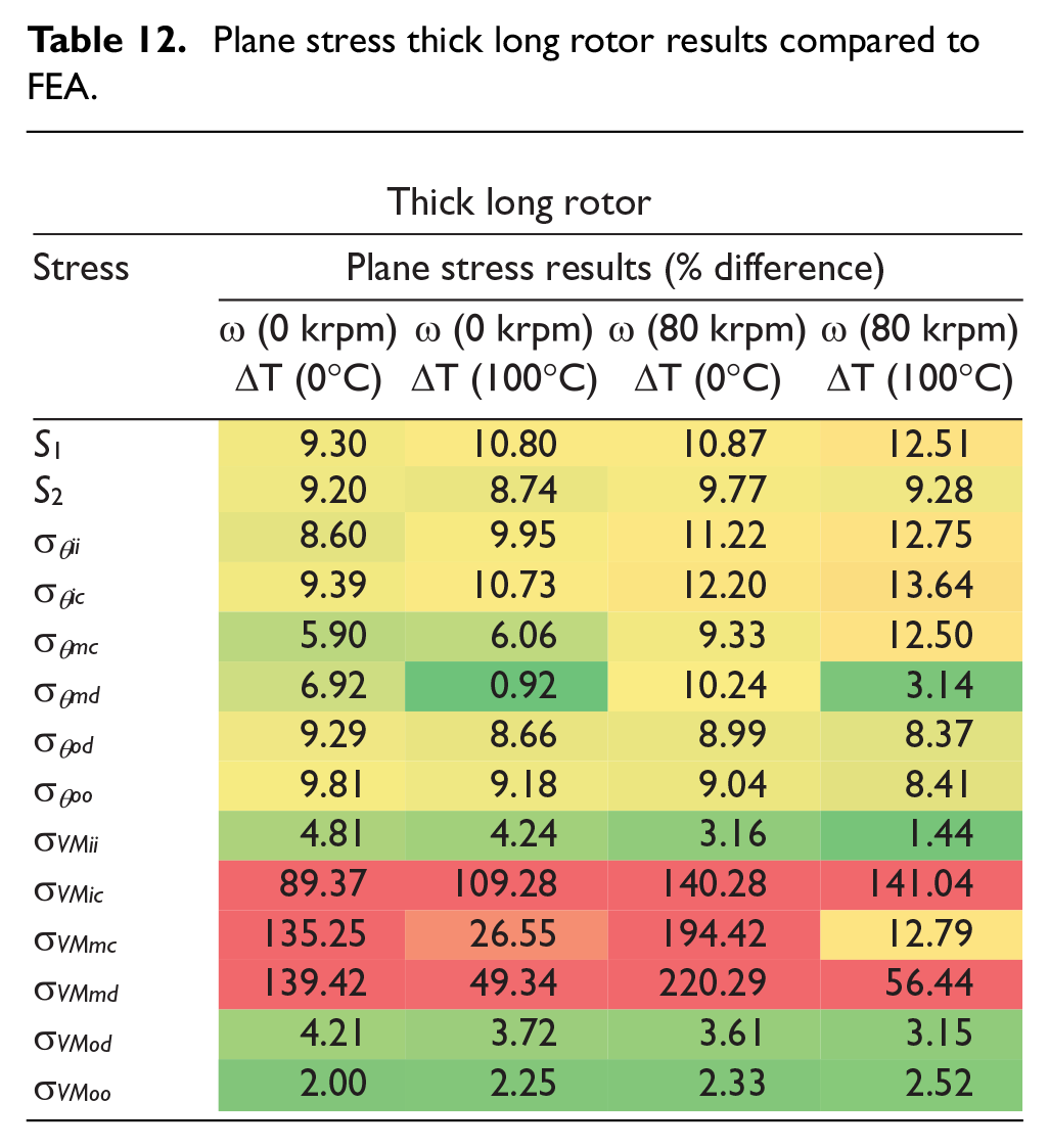
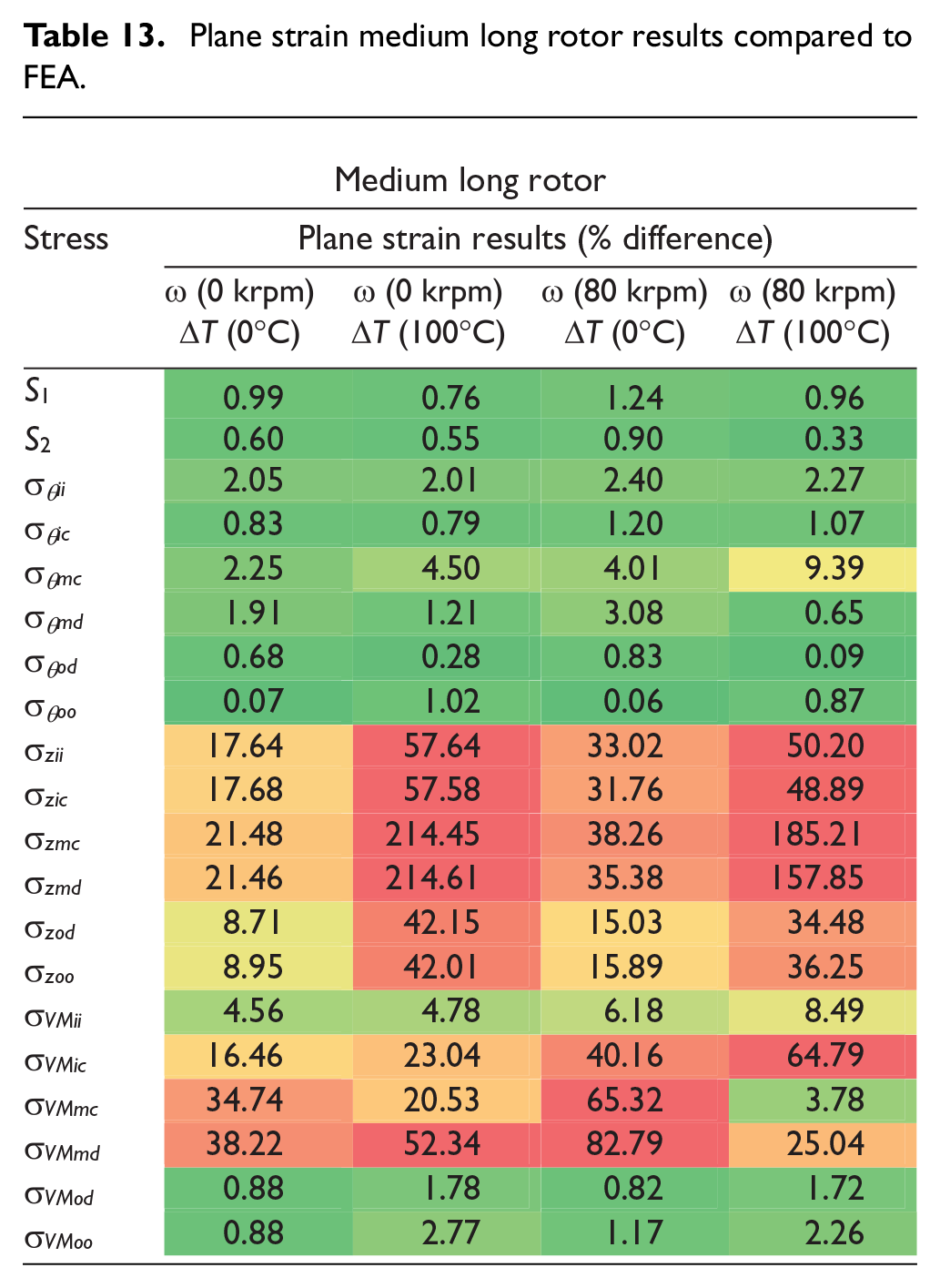
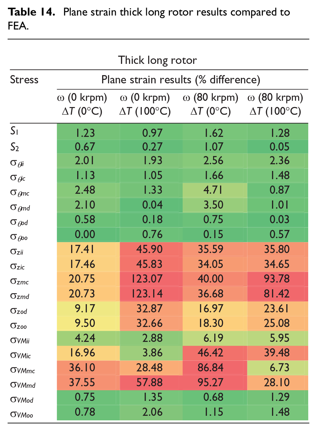
Tables 11 and 12 show the plane stress results for the medium and thick long rotors and Figure 12 compares those against the respective plane strain results from Tables 13 and 14. When comparing the GPS medium and thick long rotor results from Figure 11 to the plane stress, a similar pattern to the thin rotor results is formed. The medium and thick cylinders remaining close, but it appears that the thicker the rotor, the less accurate the results become as the thick rotor results have slightly more occurrences in the higher difference bins. The plane strain results also appear to be closely aligned, but do not follow this pattern as the thick cylinder produces a slightly more accurate result spread than the medium cylinder. This is because the inaccurate axial stress results produced by the plane strain theory, which fall in the highest difference bin, are less extreme for the thick cylinder.
Plane stress medium long rotor results compared to FEA.
Plane stress thick long rotor results compared to FEA.
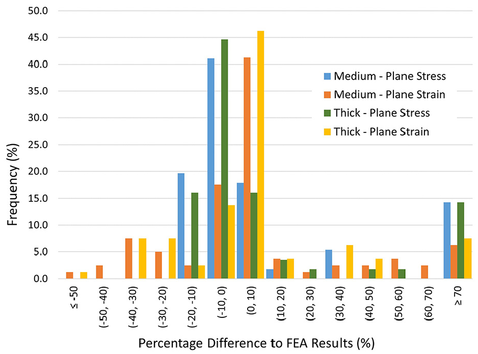
Histogram for medium and thick rotor results – plane stress and plane strain.
Plane strain medium long rotor results compared to FEA.
Plane strain thick long rotor results compared to FEA.
For the medium cylinders, only 25% of plane stress results fall within ±5% of the FEA, compared to only 53% of plane strain results falling within the same range. Neither method from Figure 12 compares to the accuracy of the GPS results shown in Figure 11, which shows 89% of results falling within ±2.5% of the FEA results.
Short rotor results
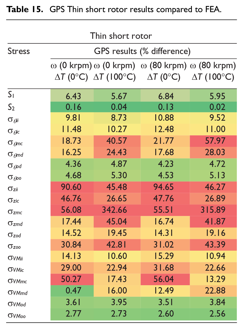
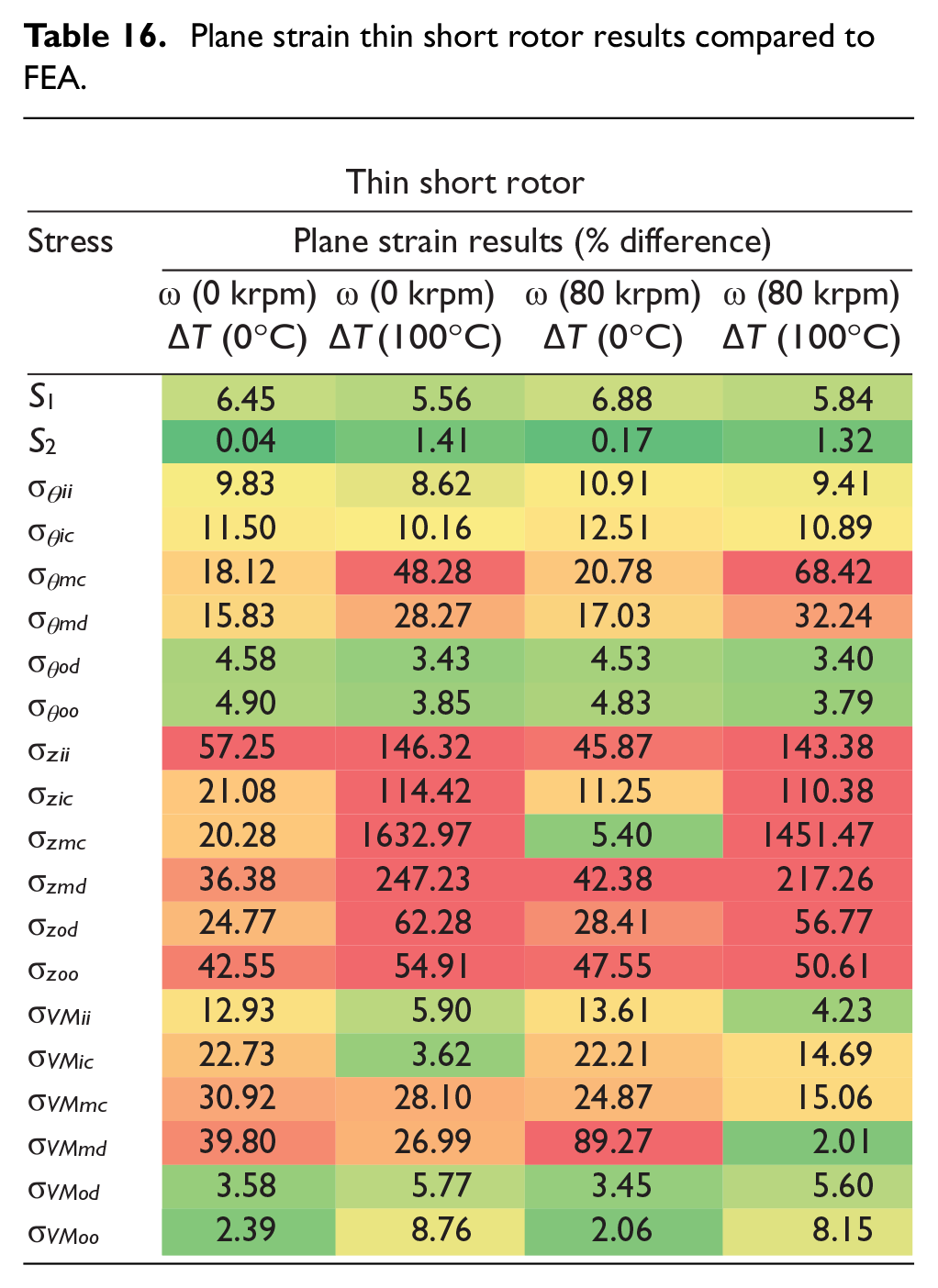
As described in the previous section, an ‘end-effect’ occurs at the rotor ends where axial stress tends to zero. This changes the rotor from a state of GPS to a state of plane stress. When analysing short rotors, it can be seen in Figure 5 that the ‘end-effect’ can affect the whole length of the rotor. The results from all analyses for the thin short rotor can be seen in Tables 15 to 17.
GPS Thin short rotor results compared to FEA.
Plane strain thin short rotor results compared to FEA.
Plane stress thin short rotor results compared to FEA.
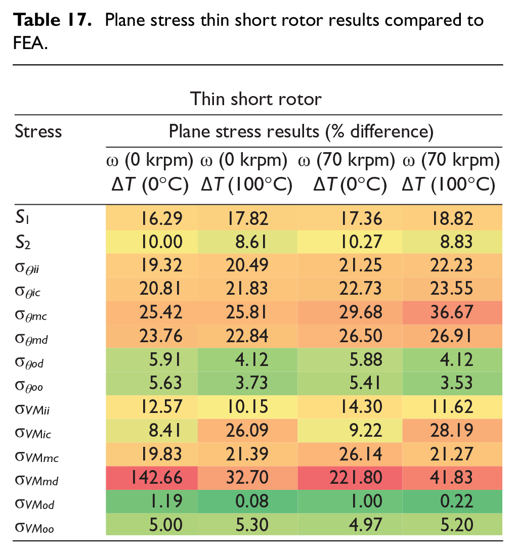
None of the theoretical approaches can be reliably used for short rotors due to being affected by the ‘end-effect’. For thin short rotors, Figure 13 shows the plane stress approach appears to have the most consistent results with less extreme outliers. This is due to the ‘end-effect’ essentially creating a state of plane stress in the rotor. Comparing Figure 13 with Figure 9, the thin long rotor results are more accurate than the thin short rotor results for plane stress, with more results concentrated in the lowest difference bins. When also compared to Figure 12, it is clear that plane stress is consistent over all tested rotor topologies. However, there are still significant errors that make the results unreliable.
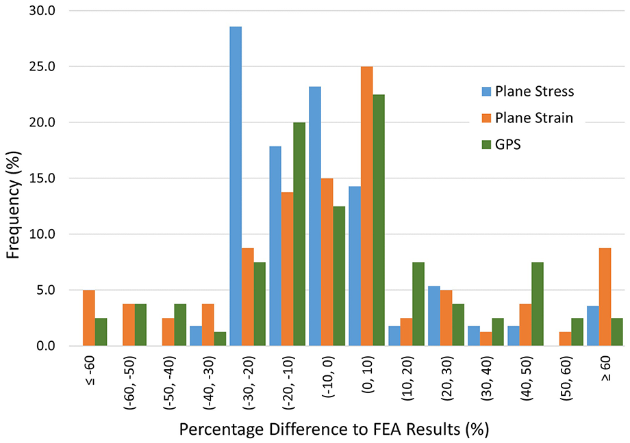
Histogram for thin short rotor results.
Plane strain appears to have a comparable distribution to GPS in Figure 13, but the major axial stress inaccuracies shown in Table 16, are concealed in the highest difference bin. Taking this into account, the GPS distribution of Table 15 has fewer occurrences in the highest difference bin and is more accurate on average than plane strain, but less accurate than plane stress. Sixty-three percent of the GPS results fall within ±20% of the FEA, however there are axial stress calculations that are significantly more inaccurate and fall outside of this range. Each theory has circa 40% of results falling outside of ±20% of the FEA. There is also no clear pattern on which results may be accurate or inaccurate.
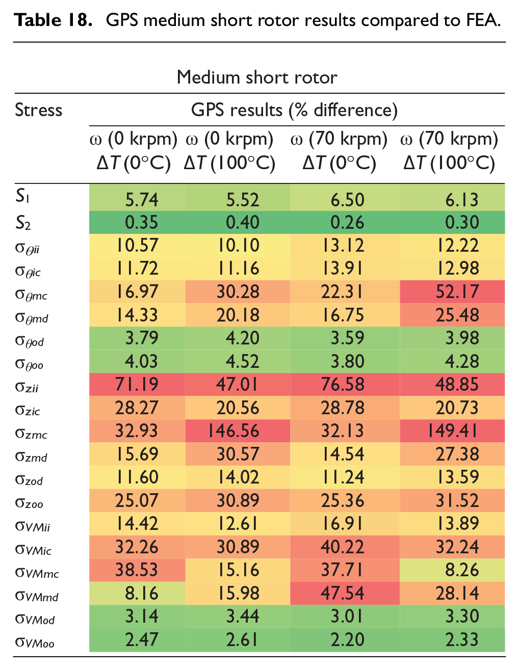
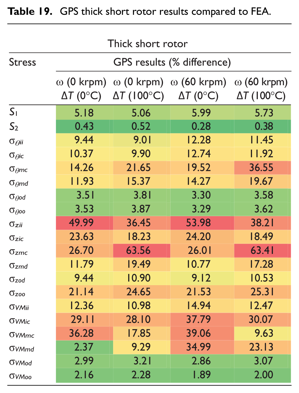
The unpredictability and unreliability in the results remains for the medium and thick short rotors, as shown by Figure 14 which uses the results data from Tables 15, 18 and 19. For the short rotors, GPS appears to increase in accuracy as the rotor thickness increases, with a higher frequency of the most accurate results and less extreme results. Mainly the axial stress results improved as rotor thickness increased.
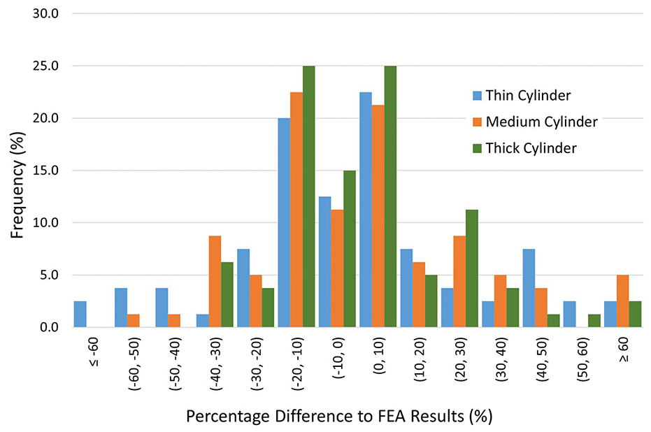
Histogram of GPS short rotor results.
GPS medium short rotor results compared to FEA.
GPS thick short rotor results compared to FEA.
Conclusion
From the results presented, it is clear that the new GPS theory is much more reliable and accurate than either plane stress or plane strain for longer rotors. It also remains accurate when temperature and or speed effects are incorporated into the calculations. The most successful GPS results were for the thin long rotor, but it was also close to the FEA results for the long medium and long thick rotors.
Most of the current research reviewed by Mallin and Barrans 12 used plane stress calculations, while a few used plane strain. Only Barrans et al. 8 had explored GPS, for two-cylinder rotors. When comparing plane strain results to the FEA, it is clear there were significant discrepancies. The axial stress calculations were severely compromised compared to the FEA, by the assumption that there was no axial strain in the rotor. These errors were then carried into the Von Mises stress calculations causing significant errors. The importance of Von Mises stress (e.g. for predicting failure of the sleeve) renders this method unreliable for the types of rotor explored in this paper.
The plane stress results were more consistent when compared against the FEA results as they didn’t fluctuate like the plane strain results. However, there were still significant differences from the FEA across all rotor topologies. These were unpredictable and caused some unreliability with the plane stress method. For long rotors, it was found that only circa 60% of plane stress results fell within ±10% of the FEA values. A 10% difference can limit rotor design or optimisation. For the same long rotors, 59% to 76% of GPS results fell within ±1% of the FEA and over 90% of results within ±3% of the FEA. This accuracy was maintained throughout rotor operating conditions and would allow rotor designs to be optimised.
There are limitations with the GPS theory. GPS results are taken from the centre of the rotor length, where the rotor is in a state of GPS. However, the rotor changes to a state of plane stress at the rotor ends. This ’end-effect’ can generate unpredictable results affecting how the rotor operates. The separation at the rotor ends shown in Figure 10 was not predicted by the GPS theory as the centre of the rotor remained in compression. It is therefore necessary to explore the ‘end-effect’ when analysing stresses in rotors. However the GPS calculations can be relied upon for great accuracy through the majority of the rotor, throughout all operating conditions.
Footnotes
Declaration of conflicting interests
The author(s) declared no potential conflicts of interest with respect to the research, authorship, and/or publication of this article.
Funding
The author(s) received no financial support for the research, authorship, and/or publication of this article.