Sage Journals: Discover world-class research

Abstract

We studied species composition and spatial distributions of tree species, and the underlying topography and soil, in subtropical forests of northwest Belize, a region in the Maya Lowlands. Our goal was to learn how much the spatial distributions of species vary and are predictable over the landscape. The study was done in old-growth, subtropical moist forest on limestone-derived topography and soil. We identified to species all trees ≥10 cm DBH in 209 400-m² plots. For each plot, we characterized topographic setting and analyzed soil nutrients and texture. We recorded 3,984 individual trees of ∼140 tree species and used the 3,775 individuals of the 69 species occurring in ≥5 plots in multivariate analyses, including Nonmetric Multidimensional Scaling (NMS). NMS showed that 73% of the variation in species composition per plot was associated with the first three ordination axes. Sixteen out of the 34 quantitative variables we measured were correlated at R² > 10% with the axes. Of the categorical variables, Topographic Class was strongly associated with species composition, and USDA Texture Class less so. Of the 69 focal tree species, the abundances of 21 were correlated at R² > 10% with one or more axes of the NMS ordination. Importantly, these 21 species accounted for 68% of all individual trees sampled in the 209 plots. Twenty-three species were indicators of particular topographic and soil classes. We conclude that patterns of tree species distribution are strongly and predictably associated with different topographic and soil conditions in this landscape. In the past, the ancient Maya could have used this type of predictable plant–soil relationship to optimize their agriculture. In the future, our results are a basis for predicting local shifts in tree species distributions due to climate change.

Keywords

subtropical forest tree species composition tree species distribution topography soil multivariate analysis indicator species Belize Maya Lowlands

Introduction

The Maya Lowlands extend from the northern end of the Yucatan Peninsula south through northern Guatemala and parts of Belize and Honduras. Research on the Lowlands’ vegetation has a long history (e.g., Bartlett, 1932), but modern quantitative studies are few in such a large region for which there is great interest in ancient Maya land use and modern management (Islebe et al., 2015). Especially informative are multivariate analyses that link data on tree species composition to data on environmental variables in forests. These analyses reveal the numerical strength of relationships between tree composition and the environment. Such results are needed for modeling the response of forest composition to changes in the environment due to disturbance and climate change (e.g., Mod et al., 2016).

In numerous studies across the tropics, the spatial distributions and abundances of a significant portion of tree species are correlated with gradients of topography and soil (reviewed in Baldeck et al., 2013). These correlations likely reflect differential adaptations among species to the variety of topographic settings and soil characteristics in forest landscapes (e.g., Brenes-Arguedas et al., 2008; Palmiotto et al., 2004). Several studies in the Maya Lowlands have described gradients of tree species on the topographic continuum but did not quantitatively link tree and environmental data (Furley and Newey, 1979; Lambert and Arnason, 1978; Lundell, 1937; Shepherd, 1975; Testé et al., 2020; Wright et al., 1959). For the Lowlands, we know of just three previous multivariate studies that do link these data, one of them unpublished (Hightower, 2012; Schulze and Whitacre, 1999; White and Hood, 2004). In this paper, we present multivariate analyses of tree species composition, soil characteristics, and topography in the varied terrain of the Rio Bravo Conservation and Management Area (RBCMA), in northwestern Belize. Our research questions were: Are tree species in the RBCMA distributed randomly, or are they distributed in predictable patterns on the landscape, and, how are tree species distributions and abundances on the landscape quantitatively associated with topographic position and/or soil characteristics?

Based on our results, we comment on how ancient Maya land use may affect the patterns we observe today, and we discuss the significance of those patterns for visualizing ancient Maya land use as a “managed mosaic,” in which the Maya tailored their land use to specific soil types and topographic settings (Fedick, 1996; Ford and Nigh, 2015). We also discuss how these quantitative results can help to predict future spatial distributions and abundances of tree species in a changing climate.

Methods

Study area

We conducted this study in the Rio Bravo Conservation and Management Area (RBCMA) in northwest Belize (Figure 1). The 100,400 ha RBCMA is managed by the Programme for Belize for biodiversity conservation, sustainable uses, and environmental education (Programme for Belize, 2022). The reserve is centered at about 17°50’ N latitude. At La Milpa Lodge in the RBCMA, the mean annual temperature for the period 2006–2014 was 25°C (Programme for Belize, 2022). Total annual rainfall averaged 1499 mm during 2006–2014, with most of the rain falling between May and December, the remaining months being significantly drier. The RBCMA is in the “subtropical moist” life zone (Holdridge Life Zone System, Hartshorn et al., 1984).

Figure 1.

Locations of the western area of the Rio Bavo Conservation and Management Area (RBCMA) and of the Chawak But’o’ob (CB) and Dos Hombres to Grand Cacao Transect (DG) study sites. The RBCMA boundary is in red; the western area is c. 34,000 ha of the 104,000 ha RBCMA. Land surface in dark green is at c. 20 m asl; surface in darker brown near Guatemala border is at c. 200 m. Inset shows approximate coverage of main map. RBCMA boundaries on the map are not official. Study sites are not to scale.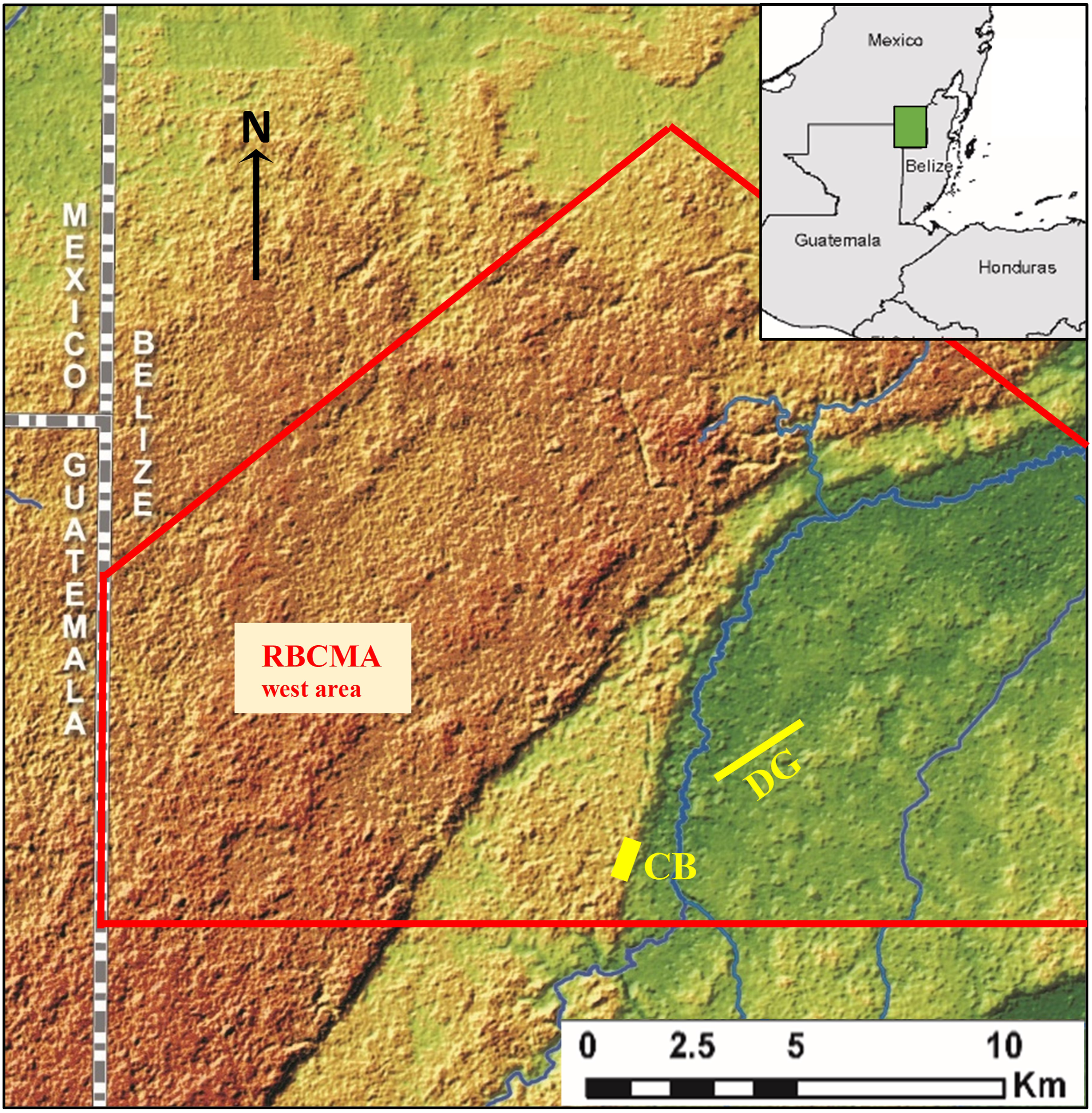

The RBCMA is on the Yucatan Platform, consisting of marine sediments consolidated during the Eocene (Dunning et al., 2003). The Platform began rising from the sea and exposing the area of northern Belize in the Pliocene. Faulting has produced escarpments 30–60 m high, and dissolution of the parent limestone and sedimentation has produced hills and valleys and gently rolling or level areas. Elevation of the RBCMA ranges from about 20 m asl in the northeast to 200 m asl near the Guatemala border. Soil parent materials are “fragmented limestone and chalk” (Wright et al., 1959).

The RBCMA has a mosaic of forest types, including upland forests on hills and other well-drained sites, with upper canopy height mainly 18–20 m and emergent trees 25–30 m tall; “bajos,” which are shallow, poorly drained basins in upland areas, with canopy 6–10 m; riparian forests with a low main canopy 10–15 m but scattered large trees to 30 m; palm-dominated forests with trees to 25 m; and transition forests among these (Brokaw et al., in review). Our study plots (Section 2.2) were mainly in upland forest, with some in transition forests between upland and poorly drained sites. The structure and composition of the RBCMA forest is similar to that of the forest at Tikal, Guatemala (96 km SW of RBCMA), described by Schulze and Whitacre (1999). Dunning et al. (2003) provide an overview of the regional environment.

Environmental history

The climate described above has prevailed since about 4,000 BC and supported subtropical forest (Frappier, 2016; Leyden, 2002). However, this forest has been subjected to hurricanes (Friesner, 1993), decades-long droughts (Hodell et al., 2005), deforestation by the ancient Maya (Beach et al., 2018; Jones, 1994), and natural reforestation after the Maya decline (Anselmetti et al., 2007). Apparently, the most recent hurricane that may have strongly affected the study area passed 65 km to the northeast in 1955 (Friesner, 1993). Hurricane Richard, in 2010, affected areas in the RBCMA but did not significantly affect the study area (Map 1 in Programme for Belize, 2022). Research nearby in Mexico shows that hurricanes typically cause dramatic structural damage but have little effect on dominant tree species composition (Navarro-Martínez et al., 2012; Vandecar et al., 2011).

Judging from land use history and from forest and soil characteristics, we believe that the RBCMA largely supports old-growth forest, having attained great age, with little disturbance. Ancient Maya activity is well-documented in the region (Guderjan, 2007; Scarborough et al., 2003), but since the abrupt decline of the local Maya, c. 950 AD (Hammond et al., 1998) there has been little human disturbance. Early logging for mahogany (Swietenia macrophylla) with axe and oxen transport would have affected a limited area (Weaver and Sabido, 1997). By the era of chainsaws and trucks, the Belize Estate & Produce Company owned the area and logged just a few tree species, causing relatively little forest damage (cf. Whitman et al., 1997). And the Company limited other uses: in 1953, there were only about 10 farming families, clustered in one area of the present RBCMA (Figure IX in Wright et al., 1959). Since the RBCMA was established in 1988 there has been no logging in our study area. During the 1980s, farmers cultivated small plots in three areas of the future reserve but not in our study area (N. Brokaw, personal observation). Present day characteristics that indicate old-growth status (Budowski, 1965) of forest in the RBCMA include (1) tall and large-diameter trees for this environment, (2) complex three-dimensional forest structure, (3) large lianas, and (4) and large fallen trees (N. Brokaw, personal observation). There are also abundant seedlings and saplings of species that will replace abundant conspecifics in the canopy, suggesting stability of species composition (unpublished data). In each of two 1-ha plots in representative upland forest in the RBCMA, eight tree species are among both the 10 most abundant upper canopy species (stems ≥10 cm DBH: diameter at breast height) and among the 10 most abundant species with stems 1–10 cm DBH. Lastly, soil characteristics also indicate old-growth forest (Beach et al., 2018).

Study sites and plots

We established two study sites in old-growth forest in the RBCMA to examine tree distributions in relation to topography and soil. The sites were at locations being mapped and excavated by archaeologists: Chawak But’o’ob and the Dos Hombres to Gran Cacao Transect. The sites are c. 3 km from each other at their closest approach (Figure 1). At both sites, we used a systematic, rather than random, arrangement of sample plots to capitalize on archaeological surveys and to more easily position and relocate points in this dense forest on sometimes steep terrain.

Chawak But’o’ob (CB) extends north–south for 1300 m along the 400-m wide slope (horizontal distance) of the east-facing Rio Bravo Escarpment. The escarpment drops 55 m at an average inclination of 13.7%, which includes steeper slopes and level benches. Near the base of the escarpment, there is an abrupt transition to the Rio Bravo floodplain. Soils are “grey brown or brown grey rocky clay loam” and “grey brown or brown grey gravelly clay loam on rocks,” according to the soil map of Wright et al. (1959). The site was occupied by ancient Maya “commoners” (Walling et al., 2020). Archaeological remains are prevalent but modest. The forest has a main canopy 18–20 m in height and emergent trees to about 25 m, about 52 tree species ha⁻¹ (among all trees ≥10 cm DBH; unpublished data), frequent lianas (large, woody vines), occasional epiphytes, and an understory with many shrubs and small palms.

At CB, we established five parallel north–south transects, each separated by 100 m. The most westerly transect was near the top of the escarpment and the easterly transect was near the escarpment base. The transects varied in length from 150 to 1300 m, to maximize coverage of the irregular shape of the escarpment face. Every 50 m along each of the transects, we established a 400-m² circular tree sample plot, for a total of 88 plots.

At the time of our study, the Dos Hombres to Gran Cacao Transect (DG) was a 2150 m long, 150 m wide “belt” transect, established for an archaeological survey conducted by M. Cortes-Rincon (McFarland and Cortes-Rincon 2019). It passed through scattered hills supporting upland forest, and low-lying terrain mainly supporting forest transitional between upland forests and bajos. Upland forest soils and forest physiognomy are similar to those described above at CB. Bajo soils are “pale brownish-grey or pale grey clay” soils that are sometimes flooded in the wet season and edaphically dry (holding water too tightly for effective plant use) in the dry season (Wright et al., 1959). The wetting and drying creates “gilgai,” a hummocky micro-relief. Bajos support a low forest of dense stems and often a sedge (Cyperaceae) ground cover. Archaeological sites are absent along most of the DG transect, but there are some small plazas with low remains (generally c. 1 m height).

At DG, we established a 400-m² circular sample plot every 50 m along the 2150 m baseline and, with a few exceptions, similar plots at 50 m distance from baseline plots at points on axes perpendicular to and on both sides of the baseline. This made 121 plots at DG and 88 at CB, for a total of 209 400-m² plots, their area summing to 8.36 ha.

Field methods

We defined a tree as a self-supporting, woody plant ≥10 cm DBH (diameter at breast height; i.e., at 130 cm along the tree stem from rooting point). (Archaeological workers did not cut trees ≥10 cm DBH.) At each plot, we counted and identified all trees whose bases were at least half inside the plot. Trees with multiple stems were counted as one individual, but all stems ≥10 cm DBH were measured. We estimated the DBH of palms that had stems sheathed in leaves. Basal area was calculated as the cross-sectional area of stems (including multiple stems), using DBH and the formula area = πr². Most trees were identified to species in the field based on experience and previously collected voucher specimens (Brokaw et al., 2021). We collected unknowns for identification.

We classified the topographic setting of each 400-m² plot as hilltop, rolling to level, slope, slope bottom (on slope but near bottom), hill base (just off slope), lowland (low-lying and level, no sign of flooding), bajo (gilgai and/or sedge evident), or floodplain (sometimes flooded). We measured the predominant inclination (degrees) of the plot (if any) with an inclinometer.

Soil sampling and analysis

We took one soil sample in each 400-m² plot, at 1 m SE of the center point. We removed the surface litter and dug a ∼20 cm wide hole, to the depth of bedrock or a maximum of 20 cm, from which we removed soil from the top to the bottom of the hole, to sample more completely the soil zone used by tree roots. We mixed the sample in the field and extracted from the mix about one cup (∼237 cc) of soil. Soil samples were air dried, complete drying being impossible under field conditions. (Remaining moisture in the samples may have limited the precision of soil parameter measurements. With more precision, we might have seen stronger associations of environmental variables with plot species composition.) We did not measure soil water since it is highly variable temporally, and thus is difficult to measure meaningfully in the field (Kursar et al., 2005).

We sent the 209 samples to the Cornell Nutrient Analysis Laboratory (Ithaca, New York) for analysis. Analysis of soil particle composition (soil texture) (Kettler et al., 2001 in Moebius-Clune et al., 2016) included determination of percent sand, silt, and clay, and USDA Soil Texture Class (USDA, 1987). Total nitrogen and total carbon were determined following Zimmerman et al. (1997). Loss on ignition (LOI) and organic matter were determined after Schulte and Hoskins (2009). The Mehlich III extraction (Mehlich, 1984; Wolf and Beegle, 2009) was used for standard nutrient analysis, which was carried out following U.S. EPA (1996).

Analysis

Our analysis followed this sequence, explained in more detail below: (1) we arranged the 209 sample plots in a primary matrix of plot species composition (presence and abundance of each tree species per plot) and a secondary matrix of the measured values of environmental variables per plot; (2) using the primary matrix we created an ordination that arrayed the sample plots along several axes in proportion to their similarity in tree species composition (comparing each plot with all other plots); (3) using the secondary matrix, we identified which quantitative environmental variables were correlated (Pearson) with the axes of the tree plot ordination; (4) we associated individual tree species abundances with the ordination axes and with the quantitative and categorical environmental variables; and (5) we determined which species were Indicator Species (strongly associated with certain categorical variable classes).

Data arrangement

Data from the two study sites were combined for analysis, because the sites were near each other in space and on the same parent material, only differing in that DG had more plots in low-lying topographic classes than did CB. For the primary matrix, we included only tree species that occurred in ≥5 of the 209 plots and that were identified at least to family level. We constructed three primary matrices, one each based on: the number of individuals, presence versus absence, or basal area, for each species in each plot.

The environmental data for the secondary matrix included 34 quantitative variables (degrees inclination, soil particle composition, and content of various nutrients) and two categorical variables (Topographic Class, USDA Soil Texture) (Table 1). The number of plots in different classes of categorical variables ranged from 2 to 84 (Table 2). We emphasize the distinction between quantitative and categorical variables because the two types of variables are analyzed differently.

Table 1.

Environmental variables included in the analysis.

Variable (unit)	Variable type	Variable (unit)	Variable type
Topographic Class	C	Chromium	Q
USDA Soil Texture	C	Copper	Q
Inclination (degrees)	Q	Iron	Q
Clay%	Q	Potassium	Q
Sand%	Q	Magnesium	Q
Silt%	Q	Manganese	Q
Total nitrogen	Q	Molybdenum	Q
Total carbon	Q	Sodium	Q
Moisture%	Q	Nickel	Q
Organic matter%^a	Q	Phosphorus	Q
pH	Q	Lead	Q
Aluminum	Q	Sulfur	Q
Arsenic	Q	Selenium	Q
Boron	Q	Silicon	Q
Barium	Q	Strontium	Q
Calcium	Q	Titanium	Q
Cadmium	Q	Vanadium	Q
Cobalt	Q	Zinc	Q

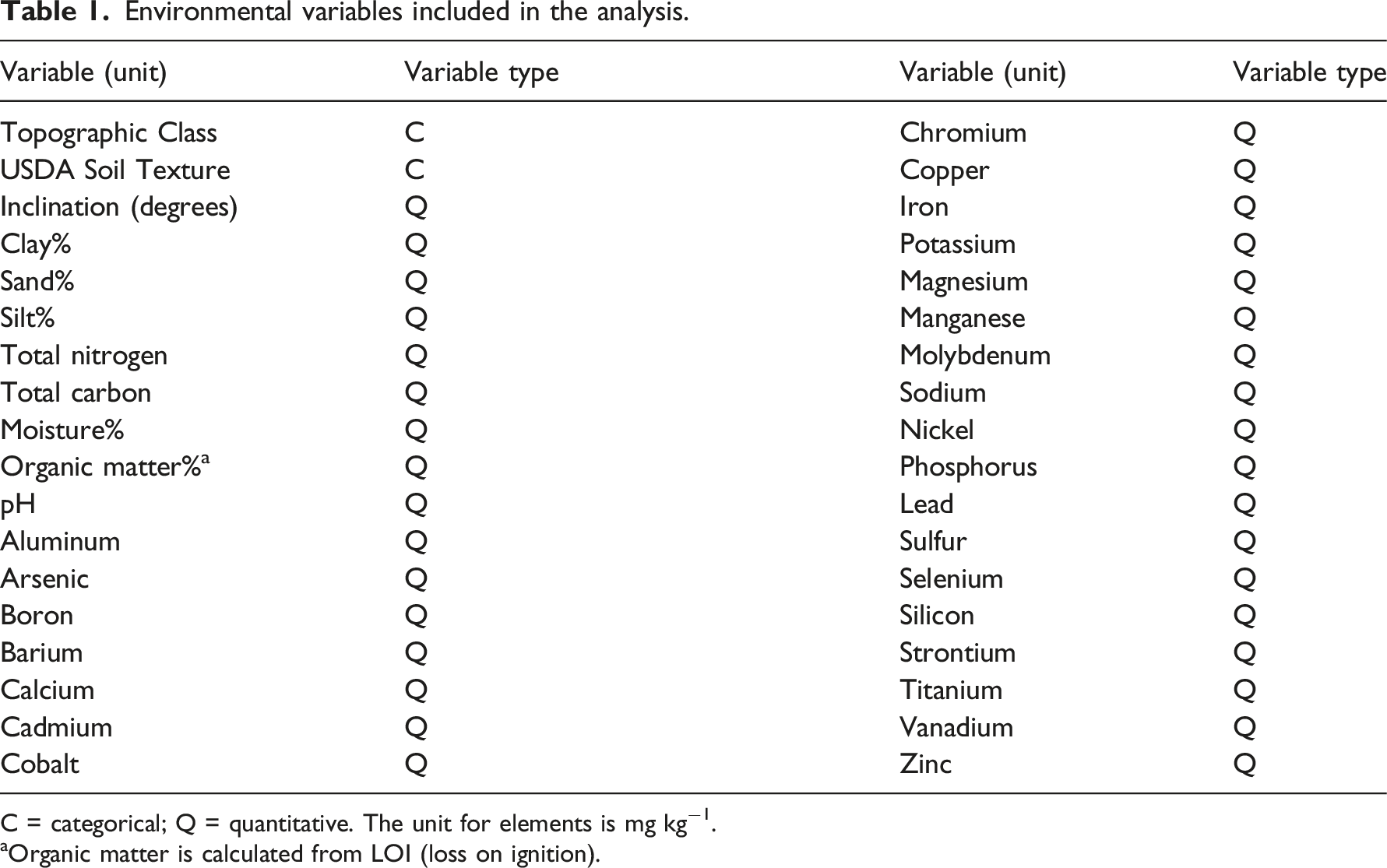
C = categorical; Q = quantitative. The unit for elements is mg kg⁻¹.

^aOrganic matter is calculated from LOI (loss on ignition).

Table 2.

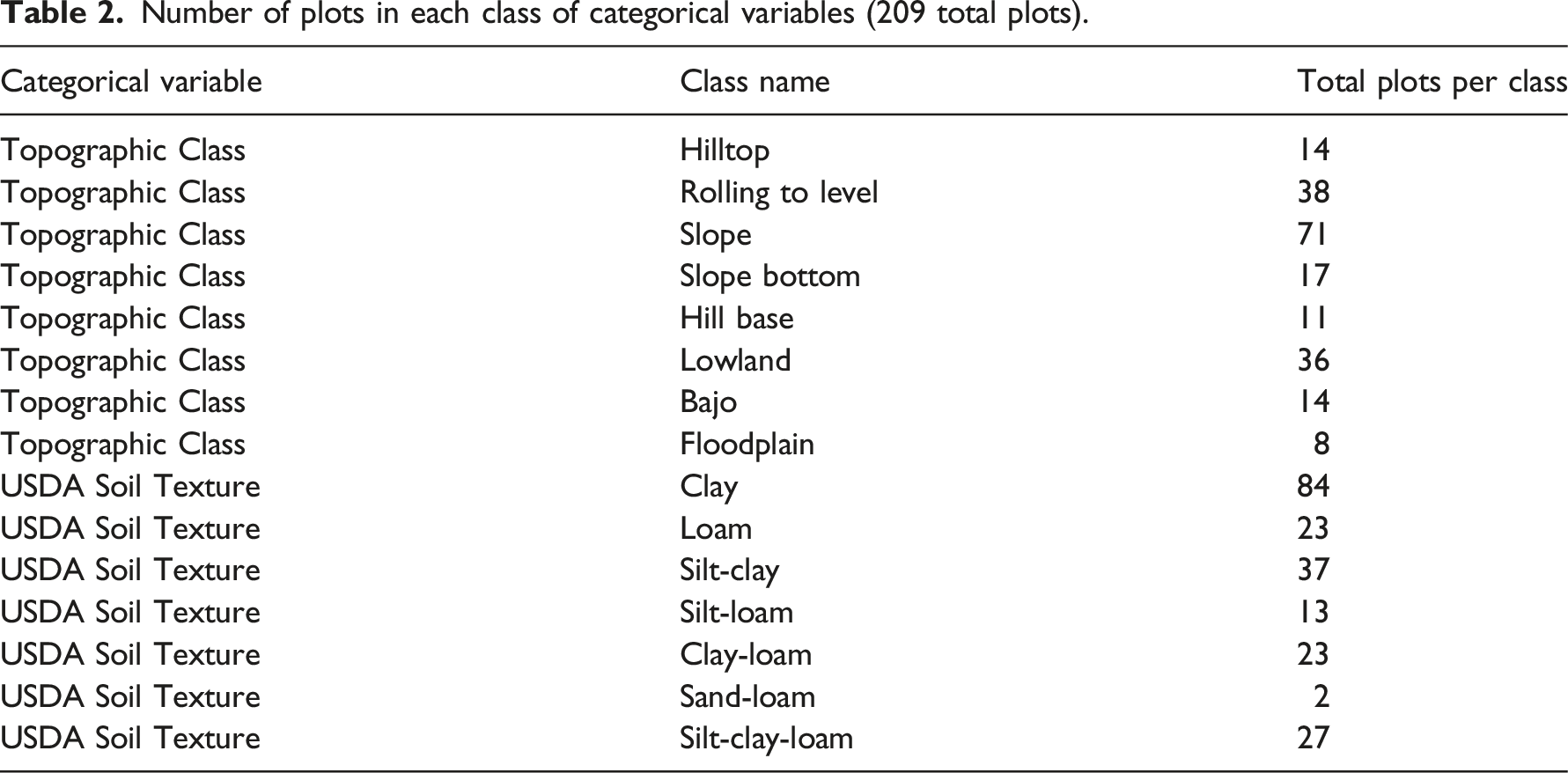
Number of plots in each class of categorical variables (209 total plots).

Categorical variable	Class name	Total plots per class
Topographic Class	Hilltop	14
Topographic Class	Rolling to level	38
Topographic Class	Slope	71
Topographic Class	Slope bottom	17
Topographic Class	Hill base	11
Topographic Class	Lowland	36
Topographic Class	Bajo	14
Topographic Class	Floodplain	8
USDA Soil Texture	Clay	84
USDA Soil Texture	Loam	23
USDA Soil Texture	Silt-clay	37
USDA Soil Texture	Silt-loam	13
USDA Soil Texture	Clay-loam	23
USDA Soil Texture	Sand-loam	2
USDA Soil Texture	Silt-clay-loam	27

Ordination of plots based on tree species composition

To determine if tree species are distributed randomly or in consistent, predictable patterns on the landscape, we created ordinations of the 209 tree plots. Ordination is a technique that arranges sample plots along axes in one or more dimensions, in proportion to plot similarity (each plot compared to all other plots) in tree species composition in primary matrices. Axes are orthogonal, that is, not correlated with each other, and represent dimensions that account for major fractions of the differences among plots. The first axis accounts for the highest proportion of variation among plots, with the second axis accounting for part of the residual variation, and so on for subsequent axes. For our ordinations, we used Nonmetric Multidimensional Scaling (NMS), which is suitable for non-normally distributed data. We used PC-ORD 7.08 (McCune and Mefford, 2018) for all ordinations in this paper.

The first step in our NMS was to determine Sørenson (Bray-Curtis) “distances” between plots (Peck, 2016), based on the degree of plot similarity in the three primary matrices: tree species composition, frequency, and basal area, respectively. The second step used these distances to perform the ordinations and determine the number and importance of axes for each of the three primary matrices.

The importance of an axis is based on the percent variation among plots accounted for by that axis, measured as R². How well the NMS ordination preserves the observed rank-order distances between plots is evaluated as “stress,” or distortion in the data (Peck, 2016), with lower values indicating less distortion. NMS performs numerous iterations of the ordination, in which one to six axes are sequentially computed and compared for the amount of variation explained and the amount of stress.

In our study, ordination based on species composition resulted in lower final stress than ordinations based on species frequency or basal area, that is, species composition provided the best association of plot distances with the axes; so we used species composition for all analyses. For the species composition data, three axes had the best combination of variation in species composition and low stress. Stress decreased from 38.009 to a minimum of 18.453, or to below 20.0, as recommended (Peck, 2016). The inclusion of a fourth axis decreased stress by 3.45, below the recommended minimum stress reduction of 5, so adding a fourth axis was not justified (Peck, 2016). We repeated the NMS ordinations based on species composition five times to verify the consistency of the stress calculations. The final stress for all five runs ranged from 18.453 to 18.459, indicating consistency of the NMS. One NMS, with final stress = 18.458, is featured in the results of this paper. The selected NMS ordination also yielded “plot scores,” that is, plot positions on each axis, to be used in further analyses.

The third step in NMS is to test whether the ordination of observed data could have been produced at random. We used a Monte Carlo test to compare the results of 250 iterations of the observed data with 249 iterations of randomized data (no penalty for ties, and using time as the random number seed [Peck, 2016]). The p value indicates the probability of obtaining a lower final stress in an iteration using randomized data (i.e., by chance alone) than using the observed data (McCune et al., 2002). A p ≤ 0.05 indicates that species composition differs significantly (is not random) among the plots.

In our ordination diagrams, the points represent the 209 plots, and the distance from one point to another in the diagram indicates the degree of similarity among plots in tree species composition (close points more similar, distant points less similar). The ordination axes can be correlated with independently measured environmental factors.

Species composition and quantitative variables

To assess the association between the primary matrix of species composition and the quantitative environmental variables in the secondary matrix (Table 1), we used a Mantel Test (Peck, 2016). Because the quantitative environmental variables were measured on different scales, we relativized their values as percent of the maximum value for each variable (0–100%). For the Mantel test, we used Sørenson distances for both the species data (primary matrix) and quantitative environmental data (secondary matrix), and we used a Monte Carlo test for significance of the association.

To further characterize the relationships between species composition and quantitative environmental variables, we also used the Mantel test to assess the strength of association between plot scores on each axis in the NMS ordination and the matrix of quantitative environmental variables. For this test, we reversed the matrices. For the primary matrix, we used Sorenson distances among plots in terms of relativized quantitative environmental variables. For the secondary matrix, we use plot scores on each axis separately. We adjusted negative values in the NMS plot scores and potential outliers by using relative Euclidean distances (Peck, 2016). We also determined the Pearson correlations (R² >10%) between individual quantitative variables per plot and each of the three axes of the NMS ordination. Tests of significance were not carried out, since with a sample size of 209 plots, correlations will be significant at a low value, possibly below ecological relevance (McCune and Grace, 2002).

Species composition and categorical variables

The association of tree species composition per plot with Topographic Class or USDA Soil Texture (Tables 1 and 2) was evaluated using Multi-response Permutation Procedure (MRPP; Peck, 2016), a non-parametric test of differences among groups (Mielke, 1984; McCune and Grace, 2002). MRPP yields A values, a statistic that describes effect size. When within-group heterogeneity equals that expected by chance, A = 0; when sample units within groups are identical, A = 1. The p value is for δ, a measure of within-group distance, which is used to calculate A (McCune and Grace, 2002). For this test, rank-transformed Sørenson distances between plots were used with the recommended weights. MRPP was also used to determine if plot scores for each axis from the NMS ordination differed among classes of the categorical variables Topographic Class and USDA Soil Texture. For these MRPPs, plot scores on axes were adjusted using relative Euclidean distances, with the recommended weights on distance (Peck, 2016).

The association between quantitative environmental variables per plot and the categorial variables of Topographic Class and USDA Soil Texture (Tables 1 and 2) were also evaluated using MRPP. The quantitative variables were relativized as described for the Mantel test, and Sørenson distances were used with the recommended weights.

Individual species analysis

We determined the Pearson correlations (R² >10%) between individual tree species abundances per plot and each of the three axes of the NMS ordination, as stated above for quantitative environmental variables.

To evaluate the association of individual tree species with the categorical variables Topographic Class and USDA Soil Texture, we used Indicator Species Analysis, based on relative abundance and constancy (Peck, 2016). Constancy is the proportion of sample units in each class in which a species occurs. Indicator values (IVs) were calculated for each species for each categorical variable class (Peck 2016) to yield a maximum IV (IVmax) among those classes (Dufrêne and Legendre, 1997). The significance of the IVmax for each species was determined with a Monte Carlo randomization test. The significance of the sum of all species IV (Sum IVmax) for a given categorical variable was also determined with a Monte Carlo test.

Results

Tree species composition among plots

Sixty-nine tree species were identified and present in ≥5 plots (Table 3). These represented 49.2% of the total number of species (69 of c.140) and 94.8% of the total individual trees (3775 of 3984) recorded in the 209 plots. For these 69 species, the selected NMS ordination showed that tree species composition was not random among the plots (Figure 2; p = 0.004). Axis 1 accounted for 39.9% of the variation in tree species abundances in the ordination, while Axis 2 accounted for 18.7% and Axis 3 for 14.5%, for a sum of 73% of the total variation in species composition.

Table 3.

The 69 tree species (stems ≥10 cm DBH and present in ≥5 of the 209 plots) used in NMS ordination tree plots in the Rio Bravo Conservation and Management Area, Belize.

Species, botanical author	Abundance	Frequency %	Basal area, m²
Alseis hondurensis Standl.	94	24	5.40
Aspidosperma cruentum Woodson	137	41	4.60
A. megalocarpon Müll. Arg.	50	20	3.50
Astronium graveolens Jacq.	36	13	1.95
Attalea cohune Mart.	24	5	2.55
Blomia prisca (Standl.) Lundell	42	16	2.84
Brosimum alicastrum Sw.	281	60	25.45
Bursera simaruba (L.) Sarg.	45	15	2.92
Calophyllum brasiliense Camb.	10	4	1.04
Cassipourea guianensis Aubl.	15	7	0.27
Cecropia peltata L.	27	9	0.46
Chrysophyllum mexicanum Brandegee ex Standl.	10	5	0.36
Coccoloba sp.	7	3	0.15
Cojoba arborea (L.) Britt. and Rose	10	5	1.29
Coussapoa oligocephala Donn. Sm.	6	2	0.75
Croton sp.	6	2	0.07
Cupania belizensis Standl.	13	5	0.35
C. rufescens Triana and Planch.	16	6	0.25
Dendropanax arboreus (L.) Decne. and Planch.	7	2	0.69
Drypetes brownii Standl.	360	59	15.76
D. lateriflora (Sw.) Krug. and Urb.	26	9	0.64
Exostema mexicanum A. Gray	6	2	0.19
Fabaceae	5	2	0.11
Ficus costaricana (Liebm.) Miq.	5	2	0.45
Ficus sp.	6	2	0.43
Guarea glabra Vahl	31	11	0.79
Guettarda combsii Urb.	16	7	0.58
Havardia albicans (Kunth) Britton and Rose	16	5	0.58
Hirtella americana L.	24	11	0.80
Laetia thamnia L.	10	4	0.18
Leptolobium panamense (Benth.) Yakoul.	21	7	0.85
Licaria peckii (Johnst.) Kosterm.	17	8	0.97
Lonchocarpus castilloi Standl.	14	6	0.81
L. luteomaculatus Pittier	7	3	0.17
Manilkara zapota (L.) van Royen	90	23	5.72
Mariosousa usumacintensis (Lundell) Seigler and Ebinger	55	22	6.69
Matayba oppositifolia (A. Rich) Britton	8	3	0.74
Melicoccus oliviformis (Kunth) Radlk.	33	14	0.95
Ottoschulzia pallida Lundell	8	4	0.44
Pimenta dioica (L.) Merrill	36	12	1.65
Pouteria amygdalina (Standl.) Baehni	107	33	7.87
P. campechiana (HBK.) Baehni	126	40	9.82
P. durlandii (Standl.) Baehni	127	37	3.19
P. reticulata (Engler) Eyma	513	76	14.78
Protium copal (Schlect. and Cham.) Engl.	108	33	4.28
Pseudolmedia spuria (Sw.) Griseb.	214	52	5.18
Quararibea funebris (Llave) Vischer	7	2	0.25
Rinorea hummellii Sprague	6	2	0.09
Rubiaceae	6	3	0.09
Sabal mauritiiformis (H. Karst.) Griseb. and H. Wendl.	301	58	7.86
Sapium lateriflorum Hemsl.	13	5	0.72
Sideroxylon foetidissimum Jacq.	62	24	4.25
Simarouba amara Aubl.	20	9	1.39
Simira salvadorensis (Standl.) Steyerm.	71	27	2.89
Spondias mombin L.	31	11	3.28
S. radlkoferi Donn. Sm.	21	9	0.93
Swartzia cubensis (Britt. and Rose) Standl.	12	5	0.72
Swietenia macrophylla King	19	8	3.33
Tabernaemontana donnell-smithii Rose	29	10	1.75
Tabebuia sp.	8	3	0.22
Terminalia amazonia (Gmel.) Exell	13	5	0.81
T. buceras (L.) C. Wright	14	5	4.81
Trichospermum lessertianum (Hochr.) Dorr	6	2	0.37
Trichilia minutiflora Standl.	160	37	2.44
Trophis racemosa (L.) Urb.	65	21	1.81
Vachellia gentlei (Standl.) Seigler and Ebinger	44	18	0.62
Vitex gaumeri Greenm.	20	8	2.74
Zanthoxylum acuminatum Sw. (Sw.)	15	6	0.84
Zuelania guidonia (Sw.) Britt. and Millsp.	7	3	0.15

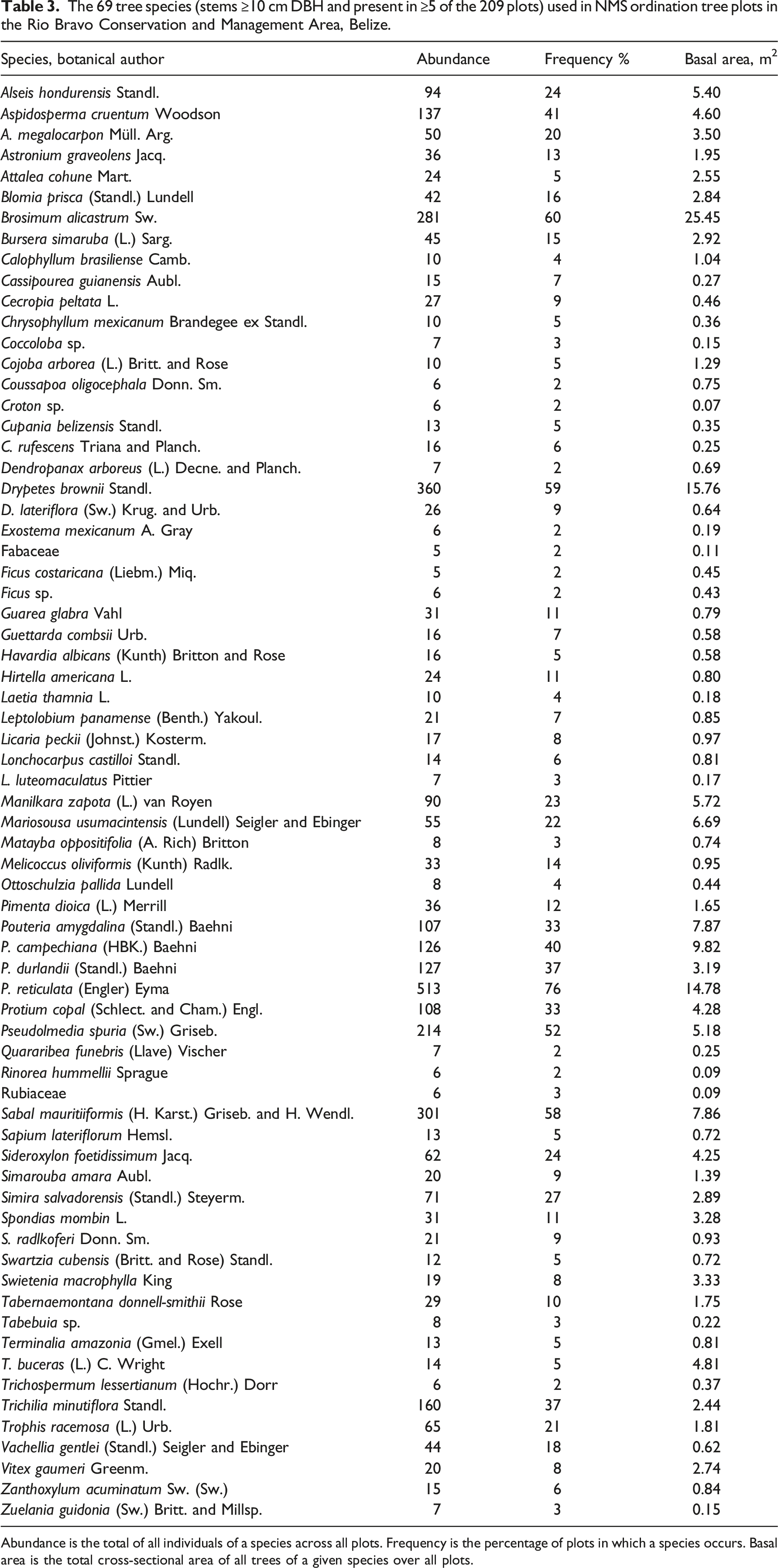
Abundance is the total of all individuals of a species across all plots. Frequency is the percentage of plots in which a species occurs. Basal area is the total cross-sectional area of all trees of a given species over all plots.

Figure 2.

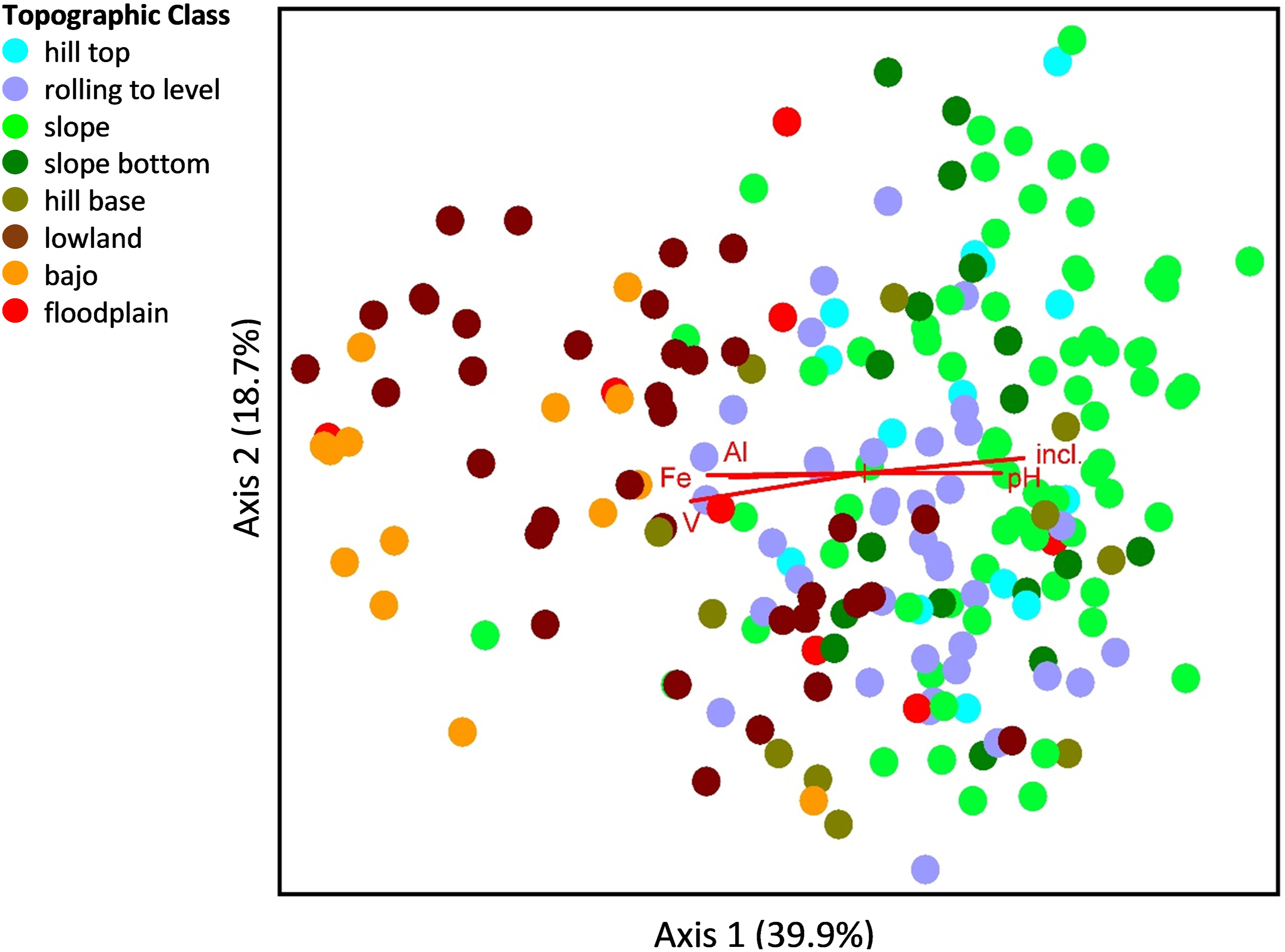
Ordination of tree species composition in 209, 400-m² plots in Belize. Each plot is shown as a dot. The dots are colored according to their Topographic Class and arranged according to their similarity in tree species composition along two axes. A gradient in species composition along Axis 1 is evidently related to the topographic gradient, from lowland and bajo on the left to hilltop and slope on the right. The red lines show the quantitative variables pH, V (vanadium), Al (aluminum), Fe (iron), and degrees inclination (incl.) that were highly correlated with Axis 1 (R² > 0.25). The percentage of variation accounted for by each axis is shown in parentheses on the axis label.

Species composition and quantitative variables

Several tests indicated strong relationships between species composition and quantitative environmental variables. In the NMS ordination, the pattern of species abundances was significantly related to the pattern of quantitative environmental variables (Standardized Mantel Statistic: r = 0.254, p for Type I error = 0.001). Other Mantel tests for the three different NMS axes showed that the matrix of relativized, quantitative environmental variables was most strongly associated with NMS plot scores on Axis 1 (Axis 1: Standardized Mantel Statistic: r = 0.184, p for Type I error = 0.001) and less so for Axis 2 (r = 0.0600, p = 0.001) and Axis 3 (r = 0.020, p = 0.017).

Almost all correlations accounting for 10% or more of the variation (R² > 0.10) between the NMS axes and individual quantitative environmental variables were with Axis 1 (15 out of the 34 quantitative environmental variables) (Table 4). The quantitative environmental variables pH, soil elements (vanadium, aluminum, and iron), and degrees inclination (overlaid on Figure 2) were significantly correlated with Axis 1 at R² > 0.25 (Table 4). Only one variable (phosphorus) was correlated at R² > 0.10 with Axis 2, and none with Axis 3. Along Axis 1 (moving from lower to higher classes on the topographic gradient) degrees inclination, pH, total carbon, total nitrogen, calcium, silt%, and titanium all increased; whereas vanadium, iron, aluminum, barium, strontium, nickel, clay%, and molybdenum all decreased (Table 4). Iron and calcium, portrayed on the NMS ordination, exemplify these patterns (Figure 3).

Table 4.

Pearson correlations (R² > 0.10) of NMS axes with relativized nutrient values, degrees inclination, and soil particle composition.

Variable	Axis	r	R ²
Vanadium	1	−0.605	0.365
Inclination	1	0.579	0.335
Iron	1	−0.577	0.333
pH	1	0.539	0.290
Aluminum	1	−0.535	0.286
Barium	1	−0.479	0.229
Total carbon	1	0.478	0.228
Strontium	1	−0.442	0.195
Total nitrogen	1	0.431	0.186
Nickel	1	−0.404	0.164
Calcium	1	0.379	0.144
Clay%	1	−0.377	0.142
Molybdenum	1	−0.371	0.138
Silt%	1	0.339	0.115
Titanium	1	0.335	0.112
Phosphorus	2	0.323	0.105

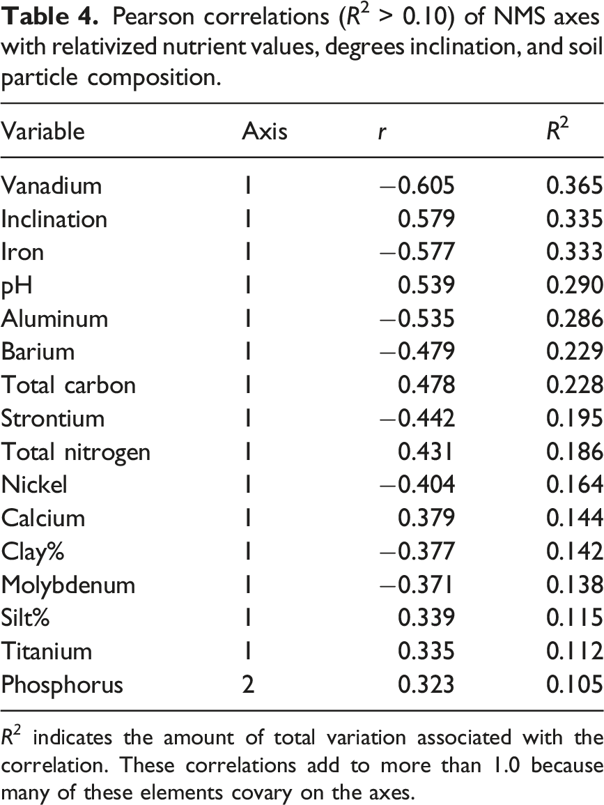
R² indicates the amount of total variation associated with the correlation. These correlations add to more than 1.0 because many of these elements covary on the axes.

Figure 3.

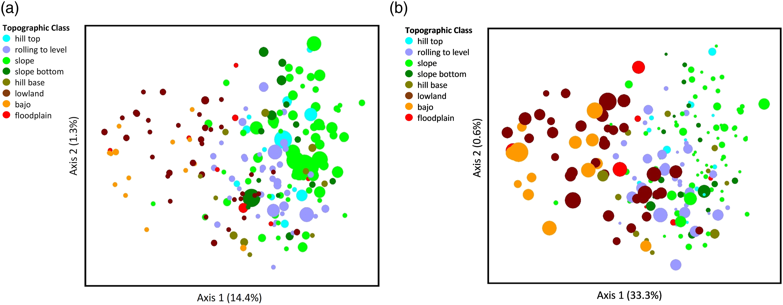
Ordination of soil elements: (a) calcium and (b) iron. The graphs depict the same ordination of plots arranged according to similarity in species composition as in Figure 2, with dots (study plots) colored according to Topographic Class. But the dots here are sized to indicate the relativized value of soil characteristics (larger dots = larger values). The amount of variation accounted for by each axis is shown as a percentage in parentheses on the axis label.

Species composition and categorical variables

Species composition was also strongly but differently associated with categorial variables. Plot scores from the NMS (based on differences in species compositions) showed stronger differentiation among Topographic Classes (A = 0.194, p < 0.001) than among USDA Soil Texture classes (A = 0.082 p < 0.001). Plot scores on individual NMS axes were also strongly associated with Topographic Class and USDA Soil Texture, with Axis 1 having the strongest associations with both categorical variables (Table 5). Overall, the NMS axes were more strongly associated with Topographic Class than with USDA Soil Texture. Separate MRPP analyses showed that the associations of quantitative environmental variables with USDA Soil Texture (A = 0.174 p < 0.001) and Topographic Class (A = 0.153, p < 0.001) were similar and significant.

Table 5.

MRPP results for association of Axes 1, 2, and 3 of the NMS ordination with categorial variables. (For explanation of the test statistic A, see Methods.)

Categorial variable	Axis	A	P
Topographic Class	1	0.434	0.000
Topographic Class	2	0.011	0.237
Topographic Class	3	0.020	0.140
USDA Soil Texture	1	0.108	0.000
USDA Soil Texture	2	0.061	0.004
USDA Soil Texture	3	−0.014	0.766

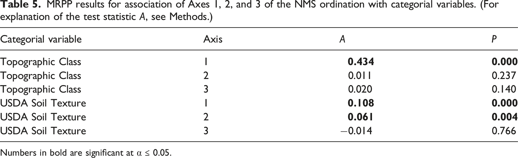
Numbers in bold are significant at α ≤ 0.05.

Individual species

Of the 69 species included in the analysis, 21 were significantly correlated (Pearson, R² > 0.10) with one or more NMS axes: 16 with Axis 1, 7 with Axis 2, and 1 species with Axis 3, and 3 were correlated with both Axes 1 and 2 (Table 6). Despite the strong correlation of Axis 3 with Pouteria reticulata, no environmental variables were strongly correlated with this axis (Table 6). These nonrandomly distributed species and individuals were 15.0% of the total number of species (21 of c.140) and 68.2% of the total individuals (2719 of 3984) recorded in the 209 plots.

Table 6.

Twenty-one species whose abundances correlated (R² > 10%) with one or more axes of NMS ordination.

Species	Axis	r	R ²
Sabal mauritiiformis	1	−0.677	0.458
Cupania rufescens	1	−0.476	0.227
Pouteria campechiana	1	0.447	0.200
Trophis racemosa	1	−0.438	0.192
Trichilia minutiflora	1	0.420	0.176
Terminalia buceras	1	−0.404	0.163
Simira salvadorensis	1	−0.402	0.162
Brosimum alicastrum	1	0.391	0.153
Swietenia macrophylla	1	−0.374	0.140
Croton sp.	1	−0.367	0.134
Drypetes brownii	1	0.342	0.117
Leptolobium panamense	1	−0.338	0.114
Pouteria amygdalina	1	0.337	0.114
Manilkara zapota	1	0.325	0.106
Blomia prisca	1	0.322	0.103
Sapium lateriflorum	1	−0.319	0.102
Pseudolmedia spuria	2	−0.537	0.288
Drypetes brownii	2	−0.536	0.287
Brosimum alicastrum	2	0.465	0.216
Pouteria durlandii	2	−0.439	0.192
Trichilia minutiflora	2	0.426	0.182
Aspidosperma cruentum	2	−0.380	0.144
Melicoccus oliviformis	2	0.380	0.144
Pouteria reticulata	3	−0.673	0.453

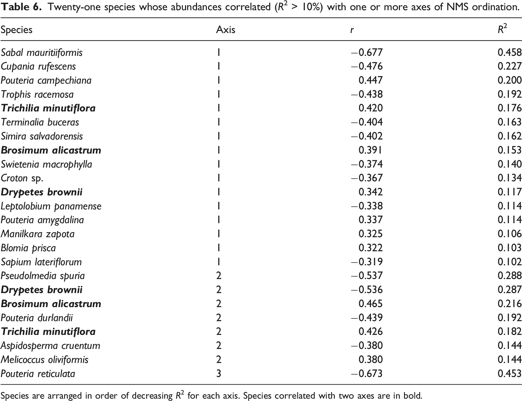
Species are arranged in order of decreasing R² for each axis. Species correlated with two axes are in bold.

Indicator Species Analysis based on categorical variables showed that 23 species were significantly associated with Topographic Class and USDA Soil Texture, based on relative abundance and constancy in each class. Seventeen species were strongly associated with particular Topographic Classes (Sum IVmax across all species = 767.94, p = 0.0002; Table 7). Six species were strongly associated with particular USDA Soil Textures (Sum IVmax across all species = 750.77, p = 0.084). Those species that were associated with USDA Soil Texture were not associated with any Topographic Class.

Table 7.

Indicator species: Tree species associated with a particular Topographic Class or with USDA Soil Texture.

Species	Topogr.	IVmax	p	Text.	IV	p
Blomia prisca	Hilltop	16.3	0.030	—	—	—
Brosimum alicastrum	Hilltop	27	0.001	—	—	—
Cassipourea guianensis	Bajo	14.7	0.022	—	—	—
Croton sp.	Bajo	26.5	0.001	—	—	—
Cupania rufescens	Bajo	31.4	0.000	—	—	—
Drypetes lateriflora	Slope	14.2	0.037	—	—	—
Guettarda combsii	—	—	—	s. loam	32.2	0.018
Havardia albicans	Lowland	17.4	0.013	—	—	—
Leptolobium panamense	Bajo	22.7	0.003	—	—	—
Lonchocarpus castilloi	Bajo	25.5	0.001	—	—	—
Manilkara zapota	—	—	—	s. loam	33.1	0.033
Melicoccus oliviformis	—	—	—	Loam	23.6	0.042
Pouteria campechiana	—	—	—	s. loam	40.2	0.022
Pouteria reticulata	Hilltop	20.1	0.022	—	—	—
Quararibea funebris	Flood.	25.3	0.001	—	—	—
Rubiaceae	—	—	—	s. loam	42.8	0.003
Sabal mauritiiformis	Lowland	23.9	0.006	—	—	—
Sapium lateriflorum	Bajo	13.2	0.034	—	—	—
Swietenia macrophylla	Bajo	12.4	0.041	—	—	—
Trichospermum lessertianum	Lowland	13.9	0.023	—	—	—
Trichilia minutiflora	Slope	19.8	0.021	—	—	—
Trophis racemosa	Bajo	32.1	0.000	—	—	—
Zanthoxylum acuminatum	—	—	—	s. loam	37.4	0.009

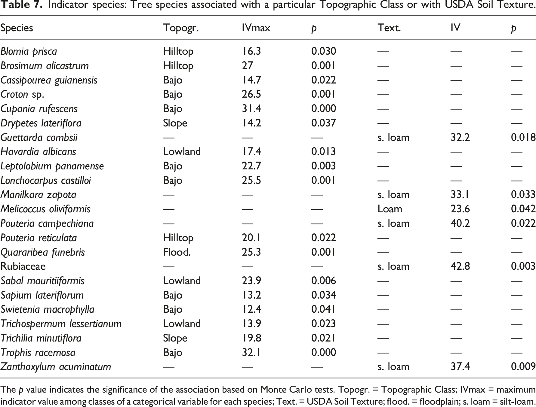
The p value indicates the significance of the association based on Monte Carlo tests. Topogr. = Topographic Class; IVmax = maximum indicator value among classes of a categorical variable for each species; Text. = USDA Soil Texture; flood. = floodplain; s. loam = silt-loam.

Three abundant species were chosen to portray contrasting patterns in the ordination (Figure 4). Brosimum alicastrum is an indicator most abundant in sites high on the topographic gradient (Figure 4(a); Sabal mauritiiformis, a palm, is an indicator more abundant lower on the gradient (Figure 4(b)); and Aspidosperma megalocarpon is not an indicator species and is more broadly distributed on the gradient (Figure 4(c)). The axes explain a substantial amount of the variation of the indicator species B. alicastrum and S. mauritiiformis but explain little of the generally distributed A. megalocarpon.

Figure 4.

Representation in ordination space of (a) Brosimum alicastrum, (b) Sabal mauritiiformis, and (c) Aspidosperma megalocarpon. The graphs depict the same ordination of plots arranged according to similarity in species composition as in Figure 2, with dots (study plots) colored according to Topographic Class. But the dots here are sized to indicate the relative abundance of three tree species in each study plot (B. alicastrum, smallest to largest dots = 0–7 individuals per plot; S. mauritiiformis, 0–9 individuals per plot; A. megalocarpon, 0–3 individuals per plot). The amount of variation accounted for by each axis is shown as a percentage in parentheses on the axis label.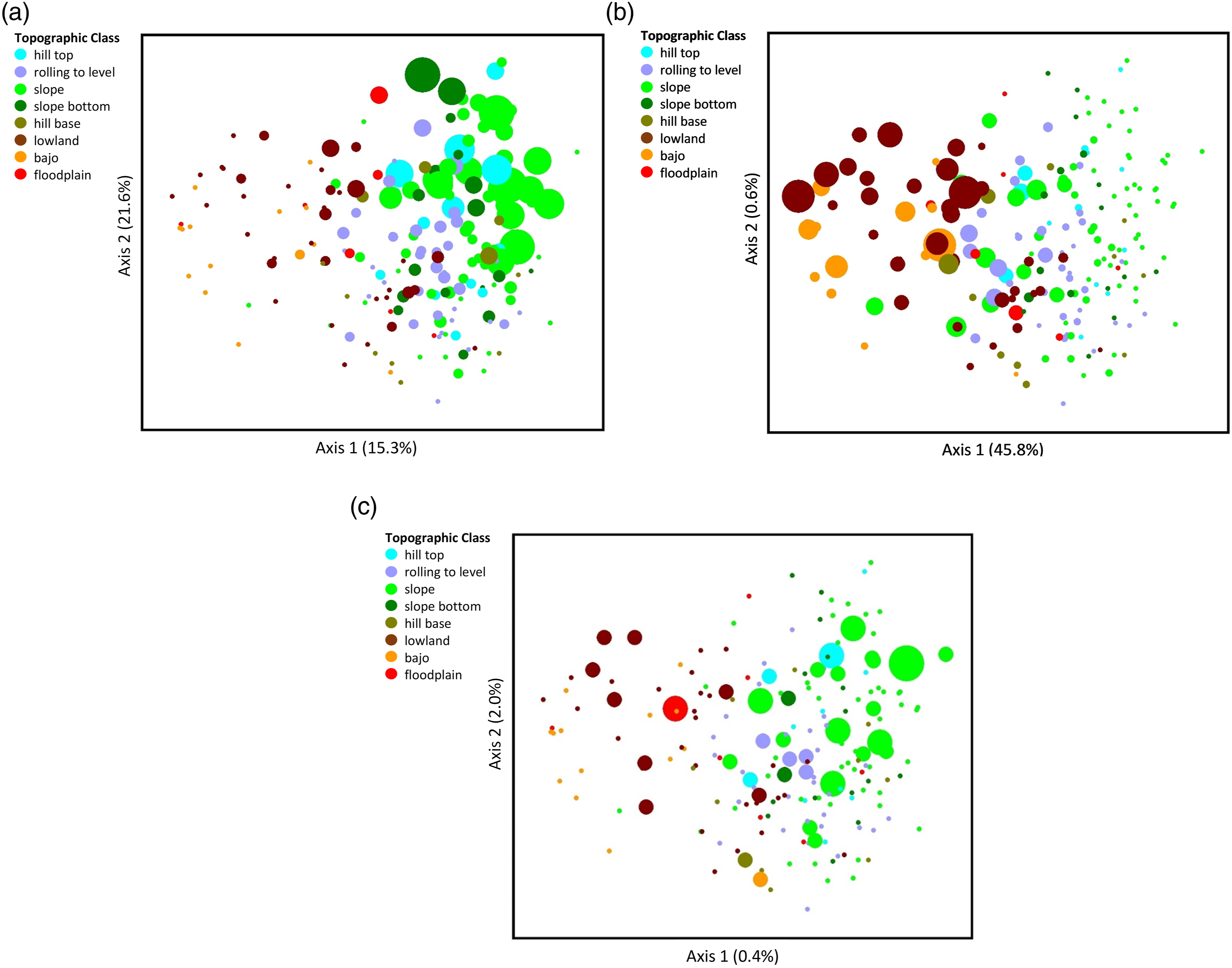

Discussion

More than 60 years ago Charles Wright described “… the remarkable correlation between the ecology of the natural vegetation on the one hand and the soil pattern on the other [in Belize]” (Wright et al., 1959). Our study supports this generalization. We found that tree species composition and the spatial distributions of many individual tree species were significantly associated with quantitative soil variables and Topographic Class in northwest Belize. Twenty-one tree species, representing 68% of all individual trees sampled in our 209 plots, exhibited consistent, non-random distributions along the three axes of the NMS ordination. Twenty-three Indicator Species were significantly associated with the categorical variables Topographic Class and USDA Soil Texture.

Mantel and MRPP tests indicated that plot species composition was strongly associated with patterns in quantitative and categorical environmental variables, both for the overall NMS analysis and for individual NMS axes. Of the variation in tree species abundances among plots, 39.9% was accounted for by Axis 1 from the NMS ordination. This axis was correlated at R² > 10% with 15 of the 34 quantitative variables we measured, the most important variables being pH, vanadium, aluminum, iron, and degrees inclination. Axis 2 accounted for 18.7% and was correlated only with phosphorus. But phosphorus is important; it limits productivity in many tropical forests (Hou et al., 2020), and its variation across the landscape could affect species composition and distribution. Axis 3 accounted for 14.5% of variation in tree abundances, and no environmental variable was correlated with it. Overall, 27% of the variation in species composition among plots was not accounted for by the NMS ordination. This remaining variation could be related to unmeasured environmental variables, small sample size of many uncommon species, stochastic effects, or unstudied biological traits and interactions.

The categorical variable, Topographic Class, was strongly associated with species composition on Axis 1. The strength of this variable reflects the fact that position along a topographic gradient is consistently associated with trends in soil moisture, depth, nutrient content, and other environmental variables (Furley and Newey, 1979). In our study, higher topographic positions had greater degrees inclination, pH, total carbon, total nitrogen, calcium, silt%, and titanium (most of these important for plant growth), and lower amounts of various elements and clay%, than did lower topographic positions (Figure 2, Table 4). Thus, the variable Topographic Class integrates different variables that are likely associated with species composition. In our study, the association of Topographic Class with species was stronger than the association of USDA Soil Texture with species. However, the associations of Topographic Class and USDA Soil Texture with quantitative soil variables were more similar. This may partly reflect the impact of soil particle composition on element or nutrient retention (Leinweber et al., 1995).

The distributions of 16 individual tree species were associated Axis 1, which in turn was associated with degrees inclination and 14 quantitative soil variables. Pouteria reticulata, the most common species on the plots, was the only species correlated with Axis 3 and had the strongest association of any species with an axis. Yet no measured environmental variable was correlated with Axis 3, suggesting that P. reticulata abundance reflects some unmeasured variable. Three species (Drypetes brownii, Brosimum alicastrum, and Trichilia minutiflora) were strongly correlated with both Axes 1 and 2, suggesting multiple environmental influences on their distributions.

Consistent with the strong association of species composition with Topographic Class, there were 17 Indicator Species associated with different Topographic Classes. Indicator Species tended to be located at the ends of the topographic gradient: in the hilltop class at the upper end (Brosimum alicastrum and Pouteria reticulata) and in bajo or lowland classes at the lower end (Havardia albicans and Sabal mauritiiformis) (Table 3). These species seem to specialize in, or are restricted by competition to, the presumably extreme conditions found at topographic end points. The six Indicator Species for USDA Soil Texture classes were not associated with any Topographic Class.

We know of four multivariate studies linking tree and environmental data in the Maya Lowlands (including ours, with the most detailed soil analysis). These four studies indicate that topography, pH, soil organic matter, key nutrients, soil depth, and clay and rock content are associated with tree species composition (Table 8). We can generalize from these studies that upper topographic positions have more basic soils, with higher content of organic matter and higher key nutrients; lower positions have more acidic soils and more of other elements, and these gradients are associated with patterns of tree species composition and tree species distributions.

Table 8.

Studies of tree species composition in the Maya Lowlands using multivariate analysis of both tree and environmental data.

Location	Analysis	Variation accounted for, number axes	Important variables	Reference
RBCMA, Belize^a	NMS	73%, 3 axes	Topography, degrees inclination, clay%, silt%, pH, total nitrogen, total carbon, calcium, other elements	Present study
Caracol, Belize^b	NMS	70%, 2 axes	Topography, organic matter, pH, bases, copper	Hightower, 2012
Across the north central Yucatan Pen., Mexico^c	DCA	61%, 2 axes	Degrees inclination, soil depth, rock%, pH, organic matter	White and Hood, 2004
Tikal, Guatemala^d	CCA	27%, 4 axes	Topography, soil depth, clay content	Schulze and Whitacre, 1999

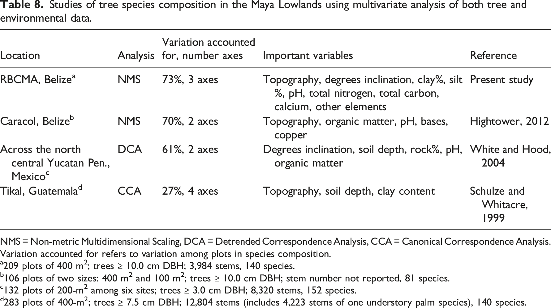
NMS = Non-metric Multidimensional Scaling, DCA = Detrended Correspondence Analysis, CCA = Canonical Correspondence Analysis. Variation accounted for refers to variation among plots in species composition.

^a209 plots of 400 m²; trees ≥ 10.0 cm DBH; 3,984 stems, 140 species.

^b106 plots of two sizes: 400 m² and 100 m²; trees ≥ 10.0 cm DBH; stem number not reported, 81 species.

^c132 plots of 200-m² among six sites; trees ≥ 3.0 cm DBH; 8,320 stems, 152 species.

^d283 plots of 400-m²; trees ≥ 7.5 cm DBH; 12,804 stems (includes 4,223 stems of one understory palm species), 140 species.

These studies (Table 8) are foundational for future research on factors that control tree species composition. So far, these studies suggest, but do not prove, that soil characteristics affect tree species distributions. To clearly determine causes of distribution, we need experiments. For example, in forests of Borneo (Born et al., 2014; Palmiotto et al., 2004) and Panama (Brenes-Arguedas et al., 2008; Kitajima, 1994), controlled field and growing-house experiments on tree seedlings revealed species-specific growth responses to variation in light, water, or nutrients that help explain species-specific distributions of adult trees in the forest. For other future studies, multivariate analysis of species and the environment can be coupled with measurements of species traits, such as “specific leaf area” and growth rate, to better understand the causes of species distributions and abundances (Meyer and Seifan, 2019).

Although we think our study sites have been free of significant human impacts for c. 1000 years, the ancient Maya were present in our area (Scarborough et al., 2003), and researchers have shown local effects of ancient Maya land use on modern tree species composition at comparable sites (Hightower, 2012; Ross, 2011; see Supplemental Material regarding a study on the Maya legacy in the RBCMA but lacking adequate design). Such an effect of ancient Maya land use would reinforce our results showing predictable tree composition, if we assume the ancient Maya farmed consistently according to topography and soil and this had persistent effects on modern tree distributions. For instance, ancient farming was closely adapted to local soil types in the Puuc region of Mexico and the Pasión region of Guatemala (Dunning, 1996), and the modern Maya of Motul de San José in Guatemala apply a detailed soil classification to their agriculture (Jensen et al., 2007). Not inconsistent with local effects of ancient land use, two studies at Tikal, both covering large areas, concluded that modern spatial distributions of tree species were largely explained by current environmental conditions (Schulze and Whitacre, 1999; Thompson et al., 2015). Either way, our study shows how predictable the effects of topography and soil are for vegetation, whether it be modern forest or ancient crops. It reveals a basis for the informed land use—a “managed mosaic” of local soils and plants—attributed to the ancient Maya (Fedick, 1996; Ford and Nigh, 2015) and which some suggest strongly contributed to their success (Demarest, 2004). Also, the predictable variation in the distributions of numerous tree species versus micro-environmental variables indicates habitat specialization, which can partly explain the richness of species in this region (e.g., Paoli et al., 2006).

While our study of the modern forest helps us visualize the environment of the ancient Maya, our quantitative results can also help us visualize a future forest shaped by climate change. “Species distribution modeling” (Franklin, 2009) can use known correlations between species distributions and environmental variables to predict future distributions under environmental change. For example, a drier climate is predicted for Central America (Hidalgo et al., 2013). This could exaggerate the comparative lack of soil water on upper slopes (García-Gamero et al., 2021), which, in turn, can affect nutrient availability (Marschner and Rengel, 2012; Viets, 1967). In particular, soil water is known to affect the availability of the key element phosphorus (O’Connell et al., 2018), and therefore possibly the distributions of species sensitive to phosphorus, along the topographic gradient. Modeling future species distributions, based on results like ours that reveal the strength of environmental associations with species distributions, can be a basis for planning agriculture and conservation.

Supplemental Material

Supplemental Material - Tree species on environmental gradients in subtropical forest of northwest Belize, in the Maya Lowlands

Supplemental Material for Tree species on environmental gradients in subtropical forest of northwest Belize, in the Maya Lowlands by Sheila E Ward, Nicholas Brokaw, Stanley Walling, and Marisol Cortes-Rincon in Progress in Physical Geography: Earth and Environment

Footnotes

Acknowledgements

Fieldwork in Belize was undertaken under a permit issued to Fred Valdez for the Programme for Belize Archaeological Project (PfBAP) by the Institute of Archaeology of the Belize National Institute of Culture and History. The Rio Bravo Conservation and Management Area (RBCMA) is managed by the Programme for Belize (PfB), a Belizean organization dedicated to tropical forest conservation, sustainable management, and environmental education. We thank PfB for permission to do research in the RBCMA and for logistical support. The PfBAP (director Fred Valdez) has been the base for our field work. Many people have helped us in the field. The authors would like to acknowledge the field directors, student interns, and volunteers of the Rio Bravo Archaeological Survey under the direction of Stanley Walling, and of the Dos Hombres-Gran Cacao Transect project directed by Marisol Cortes-Rincon, and student interns from the University of Puerto Rico and the College of St. Benedict, all of whom have contributed to this research over a number of research seasons. Thanks also go to the able field workers from the community of San Felipe, Belize, who have assisted in excavation, survey and clearing operations. We thank Elizabeth Mallory for the base map in Figure 1 and unnamed reviewers for suggesting substantial improvements to the manuscript.

Declaration of conflicting interests

The authors declared no potential conflicts of interest with respect to the research, authorship, and/or publication of this article.

Funding

The authors disclosed receipt of the following financial support for the research, authorship, and/or publication of this article: the United States National Science Foundation (DEB-1114947), United States Department of Agriculture (2017-38422-27131), and a University of Puerto Rico-Río Piedras Small Summer Grant. The research was also partly funded by a Google Arts and Heritage Grant, National Geographic Society Grant 8266-07, the Montclair State University Foundation, The Community College of Philadelphia, and the Belize Archaeology Annual Field School of Humboldt State University.

ORCID iD

Sheila E Ward

Supplemental Material

Supplemental material for this article is available online.

References

Anselmetti

Hodell

Ariztegui

, et al. (2007) Quantification of soil erosion rates related to ancient Maya deforestation. Geology 35: 915–918.

Baldeck

Harms

Yavitt

, et al. (2013) Soil resources and topography shape local tree community structure in tropical forests. Proceedings of the Royal Society B: Biological Sciences 280(1753): 20122532.

Bartlett

(1932) A biological survey of the Maya area. Bulletin of the Torrey Botanical Club 59: 7–20.

Beach

Luzzadder-Beach

Cook

, et al. (2018) Stability and instability on Maya Lowlands tropical hillslope soils. Geomorphology 305: 185208.

Born

Pluess

Burslem

, et al. (2014) Differing life history characteristics support coexistence of tree soil generalist and specialist species in tropical rain forests. Biotropica 46(1): 58–68.

Brenes-Arguedas

Marcos Ríos

Rivas-Torres

, et al. (2008) The effect of soil on the growth performance of tropical species with contrasting distributions. Oikos 117: 1453–1460.

Brokaw

Ward

Pacheco

, et al. The natural environment of northwest Belize. In review.

Brokaw

Peña-Chocarro

Knapp

, et al. (2021) Trees of La Milpa: A Field Guide to Trees of La Milpa, Rio Bravo Conservation and Management Area, Belize. Available at: https://mayaforestbelize.files.wordpress.com/2022/10/trees-of-la-milpa-ed-1-ver-8-24oct2022-1.pdf (accessed October 2022).

Budowski

(1965) Distribution of tropical American rain forest species in the light of successional processes. Turrialba 15: 40–42.

10.

Demarest

(2004) Ancient Maya: The Rise and Fall of a Rainforest Civilization. Cambridge: Cambridge University Press.

11.

Dufrêne

Legendre

(1997) Species assemblages and indicator species: the need for a flexible asymmetrical approach. Ecological Monographs 67: 345–366.

12.

Dunning

(1996) A reexamination of regional variability in the prehistoric agricultural landscape. In: Fedick

(ed) The Managed Mosaic: Ancient Maya Agriculture and Resource Use. Salt Lake City, UT: University of Utah Press.

13.

Dunning

Jones

Beach

, et al. (2003) Physiography, habitats, and landscapes of the Three Rivers Region. In: Scarborough

Valdez

Dunning

(eds) Heterarchy, Political Economy, and the Ancient Maya: The Three Rivers Region of the East-Central Yucatán Peninsula. Tucson, AZ: University of Arizona Press.

14.

Fedick

(1996) Conclusion: Landscape approaches to the study of ancient Maya Agriculture and resource use. In: Fedick

(ed.) The Managed Mosaic: Ancient Maya Agriculture and Resource Use. Salt Lake City, UT: University of Utah Press.

15.

Ford

Nigh

(2015) The Maya Forest Garden: Eight Millenia of Sustainable Cultivation of the Tropical Woodlands. Walnut Creek, CA: Left Coast Press.

16.

Franklin

(2009) Modeling Species Distributions: Spatial Inference and Prediction. Cambridge: Cambridge University Press.

17.

Frappier

(2016) Climate. In: Witschey

WRT

(ed) Encyclopedia of the Ancient Maya. Lanham, MD: Rowman & Littlefield.

18.

Friesner

(1993) Hurricanes and the Forests of Belize. Forest Planning and Management Project Occasional Series. Belmopan: Ministry of Natural Resources.

19.

Furley

Newey

(1979) Variations in plant communities with topography over tropical limestone soils. Journal of Biogeography 6: 1–15.

20.

García-Gamero

Vanwalleghem

Peña

, et al. (2022) Modelling the effect of catena position and hydrology on soil chemical weathering. SOIL 8(1): 319–335.

21.

Guderjan

(2007) The Nature of an Ancient Maya City: Resources, Interaction, and Power at Blue Creek, Belize. Tuscaloosa, AL: University of Alabama Press.

22.

Hammond

Tourtellot

Donaghey

, et al. (1998) No slow dusk: Maya urban development and decline at La Milpa, Belize. Antiquity 72: 831–837.

23.

Hartshorn

Nicolait

Hartshorn

, et al. (1984) Belize Country Environmental Profile: A Field Study. Belize City: Robert Nicolait and Associates, Ltd.

24.

Hidalgo

Amador

Alfaro

, et al. (2013) Hydrological climate change projections for Central America. Journal of Hydrology 495: 94–112.

25.

Hightower

(2012) Relating Ancient Maya Land Use Legacies to the Contemporary Forest of Caracol, Belize. Master’s Thesis, University of Central Florida, Orlando, FL.

26.

Hodell

Brenner

Curtis

(2005) Terminal classic drought in the northern Maya lowlands inferred from multiple sediment cores in Lake Chichancanab Mexico. Quaternary Science Reviews 24: 1413–1427.

27.

Hou

Luo

Kuang

. et al. (2020) Global meta-analysis shows pervasive phosphorus limitation of aboveground plant production in natural terrestrial ecosystems. Nature Communications 11(637).

28.

Islebe

Calme

León-Cortés

, et al. (eds) (2015) Biodiversity and Conservation of the Yucatán Peninsula. Switzerland: Springer International Publishing AG.

29.

Jensen

Moriarty

Johnson

, et al. (2007) Soil resources of the Motul De San José Maya: Correlating soil taxonomy and modern Itzá Maya soil classification within a classic Maya archaeological zone. Geoarchaeology: An International Journal 22: 337–357.

30.

Jones

(1994) Pollen evidence for early settlement and agriculture in northern Belize. Palynology 18: 205–211.

31.

Kettler

Doran

Gilbert

(2001) Simplified method for soil particle-size determination to accompany soil-quality analyses. Soil Science Society of America Journal 65(3): 849–852.

32.

Kitajima

(1994) Relative importance of photosynthetic traits and allocation patterns as correlates of seedling shade tolerance of 13 tropical trees. Oecologia 98: 419–428.

33.

Kursar

Engelbrecht

BMJ

Tyree

(2005) A comparison of methods for determining soil water availability in two sites in Panama with similar rainfall but distinct tree communities. Journal of Tropical Ecology 21: 297–305.

34.

Lambert

JDH

Arnason

(1978) Distribution of vegetation on Maya ruins and its relationship to ancient land-use at Lamanai, Belize. Turrialba 28: 33–41.

35.

Leinweber

Paetsch

Schulten

(1995) Heavy metal retention by organo‐mineral particle‐size fractions from soils in long‐term agricultural experiments. Acta Anaesthesiologica Scandinavica Supplementum 39(4): 271–285.

36.

Leyden

(2002) Pollen evidence for climatic variability and cultural disturbance in the Maya lowlands. Ancient Mesoamerica 13: 85–101.

37.

Lundell

(1937) The Vegetation of Petén. Washington, DC: Carnegie Institution of Washington.

38.

McCune

Mefford

(2018) PC-ORD. Multivariate Analysis of Ecological Data. Version 7.09. Corvallis, OR: Wild Blueberry Media, LLC.

39.

McCune

Grace

Urban

(2002) Analysis of Ecological Communities. Gleneden Beach, OR: MJM Software Design.

40.

McFarland

Cortes-Rincon

(2019) Mapping Maya Hinterlands: LiDAR derived visualization to identify small scale features in northwestern Belize. Humboldt Journal of Social Relations 1(41): 46–58.

41.

Marschner

Rengel

(2012) Nutrient availability in soils. In: Marschner

(ed) Marschner’s Mineral Nutrition of Higher Plants. Amsterdam: Elsevier.

42.

Mehlich

(1984) Mehlich 3 soil test extractant: A modification of Mehlich 2 extractant. Communications in Soil Science and Plant Analysis 15(12): 1409–1416.

43.

Meyer

Seifan

(2019) Trait-based modelling in ecology: A review of two decades of research. Ecological Modelling 407: 108703.

44.

Mielke

(1984) 34 Meteorological applications of permutation techniques based on distance functions. In: Handbook of Statistics. New York, NY: Elsevier Science Publishers.

45.

Mod

Scherrer

Luoto

, et al. (2016) What we use is not what we know: environmental predictors in plant distribution models. Journal of Vegetation Science 27(6): 1308–1322.

46.

Moebius-Clune

Gugino

, et al. (2016) Comprehensive Assessment of Soil Health – the Cornell Framework, Edition 3.2. Geneva, NY: College of Agriculture and Life Sciences, Cornell University.

47.

Navarro-Martínez

Durán-García

Méndez-González

(2012) El impacto del huracán Dean sobre la estructura y composición arbórea de un bosque manejado en Quintana Roo, México. Madera y Bosques 18(1): 57–76.

48.

O’Connell

Ruan

Silver

(2018) Drought drives rapid shifts in tropical rainforest soil biogeochemistry and greenhouse gas emissions. Nature Communications 9: 1348.

49.

Paoli

Curran

Zak

(2006) Soil nutrients and beta diversity in the Bornean Dipterocarpaceae: evidence for niche partitioning by tropical rain forest trees. Journal of Ecology 94: 157–170.

50.

Peck

(2016) Multivariate Analysis for Ecologists. Step-by-Step. Gleneden Beach, OR: MjM Software Design.

51.

Palmiotto

Davies

Vogt

, et al. (2004) Soil-related habitat specialization in dipterocarp rain forest tree species in Borneo. Journal of Ecology 92: 609–623.

52.

Programme for Belize (2022) Management plan 2015–2019: Rio Bravo conservation and management area. Available at: pfbelize.org (accessed October 2022).

53.

Ross

(2011) Modern tree species composition reflects ancient Maya “forest gardens” in northwest Belize. Ecological Applications 21: 75–84.

54.

Scarborough

Valdez

Dunning

(eds) (2003) Heterarchy, Political Economy, and the Ancient Maya: The Three Rivers Region of the East-Central Yucatán Peninsula. Tucson, AZ: University of Arizona Press.

55.

Schulte

Hoskins

(2009) Chapter 8: Recommended soil organic matter tests. In Recommended Soil Testing Procedures for the North Eastern USA. Newark, DE: Northeastern Regional Publication.

56.

Schulze

Whitacre

(1999) A classification and ordination of the tree community of Tikal National Park, Petén, Guatemala. Bulletin of the Florida Museum of Natural History 41: 169–297.

57.

Shepherd

(1975) The Phytosociology of a Tropical Seasonal Forest in Southeastern Mexico. Master’s Thesis, University of Wisconsin-Madison, USA.

58.

Testé

Garnier

Limondin-Lozouet

, et al. (2020) The phytoliths of Naachtun (Petén, Guatemala): Development of a modern reference for the characterization of plant communities in the Maya Tropical Lowlands. Review of Palaeobotany and Palynology 272: 104130.

59.

Thompson

Hood

Cavallaro

, et al. (2015) Connecting contemporary ecology and ethnobotany to ancient plant use practices of the Maya at Tikal. In: Lentz

Dunning

Scarborough

(eds) Tikal: Paleoecology of an Ancient Maya City. New York, NY: Cambridge University Press, pp.124–151.

60.

USDA (1987) Soil Mechanics Level 1: Module 3 - USDA Textural Soil Classification, Study Guide. United States Department of Agriculture, Soil Conservation Service.

61.

U.S. EPA (1996) Method 6010B (SW-846): Inductively Coupled Plasma-Atomic Emission Spectrometry. Washington, DC: U. S. Environmental Protection Agency.

62.

Vandecar

Lawrence

Richards

, et al. (2011) High mortality for rare species following hurricane disturbance in the southern Yucatán. Biotropica 43: 676–684.

63.

Viets

(1967) Nutrient availability in relation to soil water. In: Hagan

Haise

Edminster

(eds) Irrigation of Agricultural Lands. Hoboken, NJ: John Wiley & Sons.

64.

Walling

Hanna

Taylor

, et al. (2020) Ancient commoner agency and inter-site alignment in northwest Belize. Research Reports in Belizean Archaeology 17: 119–134.

65.

Weaver

Sabido

(1997) Mahogany in Belize: A Historical Perspective. General Technical Report IITF-2. Ashville, NC: USDA Forest Service.

66.

White

Hood

(2004) Vegetation patterns and environmental gradients in tropical dry forests of the northern Yucatan Peninsula. Journal of Vegetation Science 15: 151–160.

67.

Whitman

Brokaw

NVL

Hagan

(1997) Forest damage caused by selection logging of mahogany (Swietenia macrophylla) in northern Belize. Forest Ecology and Management 92: 87–96.

68.

Wolf

Beegle

(2009) Chapter 5: Recommended soil tests for macro and micronutrients. In Recommended Soil Testing Procedures for the North Eastern USA. Newark, DE: Northeastern Regional Publication.

69.

Wright

ACS

Romney

Arbuckle

, et al. (1959) Land in British Honduras. Surrey, United Kingdom: Her Majesty’s Stationery Office [The National Archives].

70.

Zimmerman

Keefe

Bashe

(1997) Method 4J 40.0 Determination of Carbon and Nitrogen in Sediments and Particulates of Estuarine/Coastal Waters Using Elemental Analysis. Washington, DC: U.S. Environmental Protection Agency.

Supplementary Material

Please find the following supplemental material available below.

For Open Access articles published under a Creative Commons License, all supplemental material carries the same license as the article it is associated with.

For non-Open Access articles published, all supplemental material carries a non-exclusive license, and permission requests for re-use of supplemental material or any part of supplemental material shall be sent directly to the copyright owner as specified in the copyright notice associated with the article.

0.00 MB

0.08 MB

Tree species on environmental gradients in subtropical forest of northwest Belize,in the Maya Lowlands

Abstract

Keywords

Introduction

Methods

Study area

Environmental history

Study sites and plots

Field methods

Soil sampling and analysis

Analysis

Data arrangement

Ordination of plots based on tree species composition

Species composition and quantitative variables

Species composition and categorical variables

Individual species analysis

Results

Tree species composition among plots

Species composition and quantitative variables

Species composition and categorical variables

Individual species

Discussion

Supplemental Material

Supplemental Material - Tree species on environmental gradients in subtropical forest of northwest Belize, in the Maya Lowlands

Footnotes

Acknowledgements

Declaration of conflicting interests

Funding

ORCID iD

Supplemental Material

References

Supplementary Material