
Abstract
This study aims to advance the spatial conceptualization of ‘social homophily’ by relating the match, or mismatch, between a household’s social and sociocultural characteristics and the characteristics of the neighbourhood of residence to the probability of moving away from that neighbourhood. Three matching dimensions were investigated: economic status, ethnic background and sociocultural disposition. This paper’s focus is on the sociocultural dimension because this has not been included extensively in large-scale research so far. Initially we investigate how level of education at the household level interacts with education composition at the neighbourhood level. To further investigate the sociocultural dimension, we then include the share of each partner’s income in the total household income in our analyses. Based on the spatial literature at the intersections of class, gender and family, we assume that, together with higher education, the intra-household distribution of income reflects a broader set of sociocultural values. We make use of large-N register data to analyse the residential and mobility behaviour of all registered stable couples in the four largest Dutch urban regions between 2008 and 2009. Our analyses indicate that the degree to which a household ‘matches’ its social surroundings negatively affects its probability of leaving. This is the case for all three dimensions, with sociocultural disposition having the largest effect. The conclusion reflects on the importance of these findings for social homophily, sorting and residential segregation, and proposes directions for further research.
Introduction
Notions of self-selection and self-sorting in spatial behaviour refer to the tendency of similarly disposed households to congregate, live in close proximity and make use of the same spaces. In sociological literature this has been referred to as social homophily (McPherson et al., 2001; Sampson, 2012). Often stated colloquially as ‘birds of a feather flock together’, this seems relatively straightforward in principle, yet it quickly becomes more complicated when its causes and most salient social dimensions are considered. Urban stratification studies typically focus on socioeconomic, demographic and ethnic-cultural distinctions. These have long been used to analyse the social geography of cities (e.g. Robson, 1975), as is witnessed in many residential mobility studies that seek to understand residential segregation. Indeed, several mobility studies have tried to explain the tendency towards homogeneity – through choice or constraints – as based on economic resources and ethnic backgrounds (e.g. Clark, 2017; Galster and Magnusson Turner, 2017; Ibraimovic and Masiero, 2014; Musterd et al., 2016; Smith et al., 2014). To understand residential segregation, it is important to grasp to what degree people cluster based on social traits (Fossett, 2006). We argue that such endeavours should include a major source of distinction: social cultural dispositions.
Marxist and Weberian class theory established long ago that class cannot be reduced to income and wealth (i.e. economic capital) alone; rather, it should include a distinctive sociocultural dimension. Pierre Bourdieu (1984) has argued that the upper and middle classes are fractured along sociocultural lines. Class distinctions are established, reproduced and recognized through attitudes, moral values, dispositions and consumption practices. As such, the ‘choice’ of housing and residential environment is an integral part of class dynamics. Several urban and housing studies have confirmed that there are demonstrable differences in residential behaviour and attitudes between segments of the middle class. This research emphasizes differences between the ‘new’ urban middle class and suburban-oriented middle classes, and also documents a variety of attitudes towards urban and suburban neighbourhoods (e.g., Allen, 2008; Boterman, 2012; Bridge, 2006; Butler and Robson, 2003; Hanquinet et al., 2012; Savage, 2011). Allen (2008) theorizes that fractions of the middle class tend to view urban regions as ‘space of positions’, as spatial hierarchies with neighbourhoods ranked according to respectability and desirability of their housing, amenities and population. Hence, shared knowledge and reputations are important in neighbourhood selection (also Sampson, 2012). Consequently, we expect to find spatial differences between the lower and middle classes, and between fractions of the middle class, as they distinguish themselves through both means and preferences. It is unclear, however, how sociocultural differences compare to other dimensions of residential mobility (income and ethnicity) and to what degree the sociocultural dimension produces residential patterns.
Our aim is to shed light on how sociocultural disposition – next to income and ethnicity – may contribute to sorting in residential mobility and, consequently, may sustain patterns of segregation. Cities are known to be highly dynamic, but simultaneously they are surprisingly stable in terms of stratification (Bailey et al., 2017; Sampson, 2012; Zwiers et al., 2017). Populations sort themselves into specific neighbourhoods. Using longitudinal register data, we will analyse individual-level residential behaviour within the four largest urban regions in the Netherlands. This study builds on our earlier work that focused on mobility behaviour in response to the discrepancy between an individual’s income position and that of his or her neighbourhood of residence (Musterd et al., 2016). The current study extends our inquiry into the residential tendencies towards social homogeneity by highlighting the sociocultural dimension. To the best of our knowledge, this is the first study to be based on individual register data for the integral population (not a sample) that stresses the importance of the sociocultural dimension while also controlling for other impacts. For this reason, this study seeks to contribute to new segregation research that makes use of increases in available data and computing power to compare and understand mobility and spatial sorting of social groups relatedly (e.g. Clark et al., 2014; Galster and Magnusson Turner, 2017; Hedman et al., 2011; Musterd et al., 2016).
To analyse sociocultural differences, this study will solely consider stable couples (with or without children) and will use the level of education and the type of distribution of income between partners as markers of sociocultural differentiation. Two questions will be addressed:
What is the relation between stable couples’ probability of moving out of their neighbourhood of residence and the share of couples in the neighbourhood of their own ‘type’ – that is, couples with similar sociocultural, economic or ethnic characteristics? When couples move, do they tend to move to a neighbourhood with a higher proportion of couples of their own type compared to the neighbourhood of origin?
While we analyse individual behaviour, we should note that sorting processes are not only driven by individual choices, preferences or means; they are also structured by the range of possibilities an urban region has to offer (types of housing and residential milieus), and by economic structures, housing systems, the functioning of housing markets, welfare regimes, and changes therein (Burgers and Musterd, 2002; Fossett, 2006; Tammaru et al., 2016).
The next section covers literature on sorting processes, with a particular emphasis on the sociocultural dimension. This is followed by a discussion of the data and methods used, as well as the selections made to ensure sufficient focus in the analyses. The paper ends with a discussion of the findings and a conclusion with suggestions for further research.
Literature review
Residential mobility and sorting
Seminal studies of the life course and the environment by, among others, Rossi (1955), Wolpert (1965) and Michelson (1977) have led to the development of models that seek to understand the relationships among household, environment and the decision to move (e.g. Huff and Clark, 1978). These relationships may change over time due to a range of dynamics within the household as well as in the neighbourhood, potentially resulting in some degree of ‘mismatch’ between the individual household and the neighbourhood of residence. Such a mismatch could be conducive to moving. More recently, some have proposed that residential sorting could be seen as a specific form of a broader ‘social homophily’ phenomenon. McPherson et al. (2001) argue that social homophily may include a wide range of social dimensions and domains. In terms of residential mobility, the expectation is that similarly disposed people tend to gather together in the same neighbourhoods because they are similarly embedded in housing market contexts, economic structures and social networks. Sampson (2012) argues that these spatially defined social structures are so resilient in their outcomes that neighbourhoods ‘select’ people rather than the other way around. Yet, given the variance in a wide range of social dimensions (e.g. sociocultural disposition, income ethnicity, gender, sexuality, life course), it is impossible to reside in a neighbourhood of perfect equals. This implies that not all dimensions are equally important for each social group when sorting into neighbourhoods. Moreover, for many people, and particularly for socially marginalized groups, a lack of choice may result in sorting into more heterogeneous milieus (Ibraimovic and Masiero, 2014).
In recent years, several residential mobility and segregation studies have highlighted the importance of ‘social homophily’ along various social dimensions, particularly economic and ethnic or immigrant status. Newly available individual-level register and census data allow researchers to follow individual households in greater detail and to compare households’ characteristics with those of their neighbourhoods. Using Swedish register data, Hedman et al. (2011) have found strong indications that demographic, economic and ethnic sorting take place simultaneously. Other studies have paid closer attention to the socioeconomic or ethnic dimensions of homophily in sorting. Musterd et al. (2016) used individual-level longitudinal data to measure the gap between an individual’s income position and that of the residential neighbourhood; they connected that gap with the probability of moving and also analysed the extent of the mismatch before and after the move (see also Clark et al., 2014; Galster and Magnusson Turner, 2017). The relation between an individual’s economic status and that of the neighbourhood may become more evident in later life, as parental support may allow relatively poor young adults to live in more affluent areas, and the intergenerational transfer of housing wealth may reproduce spatial patterns (Van Ham et al., 2014). Like studies of economic status, some studies of household–neighbourhood matching have focused on households that belong to specific ethnic or immigrant groups (e.g. Clark, 2002, 2017; Massey, 1985; Sampson and Sharkey, 2008). Recently, Górny and Toruńczyk-Ruiz (2014) found that, in six European cities, there was a negative association between ethnic diversity and neighbourhood attachment, which is suggestive of forces leading to ‘ethnic homophily’. Smith et al. (2014) confirmed this finding for the USA. Looking at a 20-year period, they found stable rates of spatial sorting for race. Although the identified trends may be related to choice, they are also likely the result of constraining factors related to housing accessibility and discrimination (Burgers and Musterd, 2002; Fossett, 2006).
Sociocultural dimension
Next to income and ethnic differences, the current study seeks to highlight the role of sociocultural differences in residential sorting. Although it has received considerably less attention in residential mobility studies, the sociocultural dimension is potentially very important in spatial orientations. For the purpose of our study, we highlight two elements of this dimension: the amount of cultural capital households possess, here expressed by the level of education; and whether a household arrangement of income-earning is more ‘traditional’ or ‘modern’.
Regardless of class, the neighbourhood of residence is a matter of efficient time-space strategies, housing affordability and quality (Pinkster, 2014); however, for some fractions of the middle class, it may have a broader social significance. For these groups, neighbourhood preference is influenced by easy access to cultural amenities and services, which are often located in city centres. Urban living and cultural consumption not only fulfil residents’ needs and preferences for (more) cultural capital, but also serve as a way to demonstrate distinction (Allen, 2008; see also Bridge, 2006; Butler and Robson, 2003).
While a good indicator of class, education alone is insufficient to assess the spatiality of sociocultural dispositions. Not only because it correlates with economic status, but also because it does not allow differentiation within the middle classes. Yet, the interplay between class and space is also tied to economic household arrangements.
In his study of labour, Ray Pahl (1984) noted that vast amounts of work are being carried out in the domestic sphere. In addition to formal employment, households engage in home maintenance, self-provisioning and domestic labour. Pahl’s work contributed to a growing awareness of the diversity in work which was due to ‘socio-cultural changes’ in gender relations and in consumption (Warde, 1990). Since then, economists, sociologists and geographers have studied how households divide their labour. Overall, these studies have shown that decision-making on ‘work strategies’ cannot be reduced to economic rationalism (i.e. optimum outcomes), but is also structured by local labour markets, gender relations and time-space constraints.
First, household strategies are contingent on opportunities for women to work. Employers have to accept women, but also the availability of part-time work may allow for new arrangements (Warde, 1990; Winslow-Bowe, 2009). With the advent of part-time work and service-sector jobs, often concentrated in urban centres, more women have entered the labour market in Western Europe, yet full-time employment is often still lagging (see Thévenon, 2013).
Second, arrangements between different-sex partners are influenced by gendered expectations with regard to work. Yet, these are not the only explanations for gender differences. One partner tends to focus on housework when earnings are skewed (‘bargaining and exchange theory’; Bittman et al., 2003). Multiple studies have found that women who earn less reduce paid work hours over time, leading to ‘traditional’ arrangements. Yet, when women earn more, they tend to reduce work hours over time, and men do not do more housework; here, ‘gender trumps money’ (Bittman et al., 2003; see also Bertrand et al., 2015; Brines, 1994). A Dutch study by Stam et al. (2014) indicated that women’s decisions to work fewer hours or stop working are positively related to holding traditional gender role values. Given the few structural constraints for female labour participation, these authors underscore the role of sociocultural dispositions related to ‘moral views about the ideal division of tasks between men and women within a family, pointing at a male provider role and a female caring role’ (Stam et al., 2014: 594). These findings indicate the potency of traditional norms and values. Yet, men’s and women’s ‘gender ideology’ are important in non-traditional, or ‘modern’, arrangements. Egalitarian values have an effect on amount of working hours and distribution of earnings (Presser, 1994). These values are also related to class – particularly, middle-class women are less likely to do house work than working-class women (Perry-Jenkins and Folk, 1994; see also Legerski and Cornwall, 2010). Within class, we may see differences as well (see below).
Third, distribution of work is also contingent on time-space constraints. ‘Modern’ household arrangements require specific coping strategies, affecting their geography. Residential locations that allow smooth commuting and reduce the time spent on home-to-work trips as well as the accessibility and proximity of supportive services and amenities are important for dual-income households (Boterman and Karsten, 2014). Choosing a neighbourhood of residence is a spatial strategy for addressing time-space management issues, particularly in conjunction with family life (Jarvis, 2005; Schwanen, 2007). Context is important here. A study of middle-class households in Amsterdam and London indicated that Dutch households have more opportunities for ‘modern’ arrangements. The close-knit urban fabric offered housing and facilitated everyday mobility. Furthermore, the institutional context makes part-time work possible and child care affordable (Boterman and Bridge, 2015).
The importance of residential environments for household arrangements has been noted in view of class. Early accounts of gentrification have highlighted the steady increase in women gaining access to employment and developing professional careers as a driving force behind gentrification. Increased labour market participation has meant more single women working and more couples with dual incomes. These groups preferred urban neighbourhoods rather than suburban areas, as the city gave access to employment and allowed for effective time-space management (Bondi, 1999; Karsten, 2003; Rose, 1984). Yet, Butler and Hamnett (1994) note that female labour participation and modern arrangements alone are insufficient to understand residential behaviour. Circling back to class and consumption, they argue that ‘female gentrifiers (and their male counterparts and partners) are part of a particular fraction of the middle class, with specific cultural practices’ (Butler and Hamnett, 1994: 477; see also Boterman, 2012).
Data and methods
We make use of the System of Social Statistical Datasets from Statistics Netherlands. This database consists of longitudinal integral data at the individual level for each registered resident of the Netherlands from 1999 onwards. This study uses data from two reference dates: the end of September 2008 and the end of September 2009. This coincided with the start of the financial crisis in the Netherlands, leading to a sharp decline in housing prices and sales. While the low point of the crisis did not occur until 2014, the situation had a dampening effect on residential mobility (Hochstenbach et al. 2018). However, due to Dutch mortgage regulations, hardly any moves were caused by foreclosures. The analytical focus is on the residential behaviour of opposite-sex cohabiting couples (both married and unmarried, with or without children) who were living in the four largest urban regions of the Netherlands (Amsterdam, Rotterdam, The Hague and Utrecht) on both reference dates. Our study looks at urban regions as defined by Statistics Netherlands because they align better with housing market areas. The urban regions form the so-called Randstad, the most urbanized western part of the Netherlands, which is also the key economic area of the country (see maps in the Supplemental Material).
We investigate residential moves within the urban region. Moves outside the urban region are excluded from the analysis; they are considered long-distance moves, which are more likely related to economic or educational reasons. Conversely, short-distance residential moves are more likely to be influenced by household characteristics, housing quality, neighbourhood composition and housing markets (Musterd et al., 2016). Additionally, within the urban region, the existence of local social ties, as well as more knowledge and better understanding of the region’s neighbourhood structure, may exert an influence on mobility flows between neighbourhoods (Sampson, 2012).
Moves related to life course events (household formation and dissolution) are not the focus of this study and may distort our findings. To rigorously control for life course-induced moves, we limited our study population to stable couples who were cohabiting on both reference dates. The data included people who did not move (93.8%), people who moved within the neighbourhood (0.9%), people who moved within the four urban regions (4.0%) and people who moved out of these regions (1.3%).
We limited the analysis to couples in which both partners were aged 25–48. We excluded young adults because they may not have finished their education and their residential situation tends to be more reflective of parental support than of their own economic situation (Hochstenbach and Boterman, 2017). The 48-year age cut-off point is related to data availability concerning educational level. Same-sex couples had to be excluded because of our operationalization of sociocultural categories. For the variables age and ethnicity, within each household, one adult person was randomly selected to serve as a reference person for that household. Individuals living in institutions or in large non-family households, such as student housing, were excluded.
We used statistical neighbourhoods as defined by municipalities and Statistics Netherlands based on some level of physical or social homogeneity. Their population numbers varied from 1 to 13,500 households, with an average of 1300 households per neighbourhood. Neighbourhoods with fewer than 100 households (20% of the neighbourhoods) were excluded to avoid fluctuations in social compositions. The dependent variable was split into two categories:
moves within the urban region but outside the neighbourhood; and moves within the neighbourhood or not moving (reference category)
Our main question of interest was whether a better ‘match’ with the neighbourhood leads to a lower probability of moving. We constructed three key independent variables that reflect the match between a couple and their neighbourhood in 2008 along three dimensions.
Sociocultural match
The main variable of interest for this study was the sociocultural match. Research on sociocultural orientations typically measures attitudes, tastes, lifestyles and stated preferences through the use of interviews and surveys (notably Bourdieu, 1984). Information on stated preferences is, however, not included in the register datasets. Given the nature of the data, we therefore operationalize the sociocultural dimension through two concepts: the level of education, and the balance between partners in the household regarding the share of income earned. We will first analyse how education at the household level interacts with the share of highly educated individuals in the neighbourhood and then relates to mobility behaviour. To further refine our analysis of the sociocultural dimension and differentiate from the economic, we have categorized five sociocultural categories that reflect sociocultural differentiation in the Netherlands:
Not active: neither partner has paid work. Traditional, not highly educated: neither partner is highly educated. Male partner earns 60% or more of the combined wages of the partners. Modern, not highly educated: neither partner is highly educated. Male partner earns less than 60% of the combined wages of the partners. Traditional, highly educated: one or both partners are highly educated (degree at university or higher vocational education; HBO and WO).
1
Male partner earns 60% or more of the combined wages of the partners. Modern, highly educated: one or both partners are highly educated. Male partner earns 60% or less of the combined wages of the partners.
2
For each couple, the sociocultural match was defined as the percentage of couples within the neighbourhood belonging to the same sociocultural group as the couple themselves, out of the total number of households in the neighbourhood. We should note that our use of labels such as ‘modern’ or ‘traditional’ does not imply that these categories are more or less preferable or advanced. Dual-income households may also experience their situation as a necessity. This may be particularly true for lower educated partners, who are more likely to require high levels of labour market participation to make ends meet.
3
Income and ethnicity match
The second ‘neighbourhood match’ variable was the income match variable. Household incomes of couples were categorized into four quartiles. For each couple, the income match was defined as the percentage of couples within the neighbourhood belonging to the same income quartile as the couple themselves, out of the total number of households in the neighbourhood. Household income was calculated as the equivalized yearly income of households – the spendable income as defined by Statistics Netherlands, corrected for number of household members. 4
The third ‘neighbourhood match’ variable was the ethnicity match variable. For each couple, the ethnicity match was defined as the percentage of couples within the neighbourhood belonging to the same ethnicity as the reference person in the couple, out of the total number of households in the neighbourhood. As a proxy for ethnicity, we used the country of origin of the parents, collapsed into six categories representing the four major immigrant groups in the Netherlands (Turkey, Morocco, Surinam, (former) Dutch Antilles) and others, divided into other non-Western countries and Western countries.
The denominator of the three ‘neighbourhood match’ variables consisted of the total number of households. This variable design best reflects the actual chances of a resident encountering a member of that group. However, using the total number of households means that the sociocultural match variable is influenced by residents who are excluded from the study population of stable couples: most notably, singles and people under 25 or over 48 years of age. If people select neighbourhoods based on their age composition or household composition, this would lead to an overestimation of the effect of the sociocultural match. 5 To address this potential problem, we included the percentage of singles in the neighbourhood as well as the percentage of residents within their own age group (25–29; 30–34; 35–39; 40–48) as control variables.
Other variables
We also included a series of control variables (measured in 2008 unless otherwise noted) that are known or likely to play a role in the residential mobility process and its underlying motives: age group (25–29; 30–34; 35–39; 40–48) and ethnicity (of the reference person); household income in quartiles; sociocultural group to which the couple belonged; housing tenure (own or rent); household status regarding children (presence or absence, age, transitions from childless household to household with child and vice versa); and whether someone lived in the core municipality or in one of the surrounding areas within the urban region. The control variable ‘mismatch income/housing’ represented the level of mismatch between the household income and the housing value (Musterd et al., 2016). 6 This variable has been shown to be highly relevant in residential mobility research where matching between neighbourhoods and individuals is the key independent variable, because people often move in order to match the quality of their house to their income. It is important to correct for this. The variable is defined as the household income divided by the value of the dwelling, in 10 categories, with equal numbers of households 7 in each category (deciles). Households in the low deciles live in relatively expensive dwellings 8 compared to their household income and compared to other urban households. Households in the high deciles live in relatively inexpensive dwellings. Households in the highest and lowest deciles may have a relatively higher probability of moving, the former because they may seek better-quality housing, and the latter out of necessity if they cannot afford to remain in their dwelling.
To answer our main research question about the influence of the share of ‘own group’ on the probability of moving, we used mixed-effects logistic regression models with random intercepts for neighbourhood units. 9 The first model included only the controls; the second model looked at the share of highly educated individuals at the neighbourhood level and its interaction with household education; the third model introduced our social cultural categorization at the household level; in the fourth model, the main independent variable ‘percentage of own sociocultural group in neighbourhood’ was added; and the fifth full model contained all controls and all three neighbourhood match variables. We also present a sixth model, in which we add the income distance to the neighbourhood median as another neighbourhood match variable. The impact of this variable was the central focus in Musterd et al. (2016). Adding this variable, while maintaining the ‘percentage of own group’ variables for sociocultural, income and ethnic groups, allows us to investigate how these neighbourhood match variables behave in the model when included together.
Findings
Table 1 shows the descriptives for our sample of couples. Couples in which neither partner is highly educated constitute the majority. About half are ‘traditional’ (30.6%) and half are ‘modern’ (31.1%). Among couples with at least one highly educated partner, there are slightly more ‘modern’ couples (19.1%) than ‘traditional’ couples (15.4%).
Descriptive data of research population, stable couples, 2008
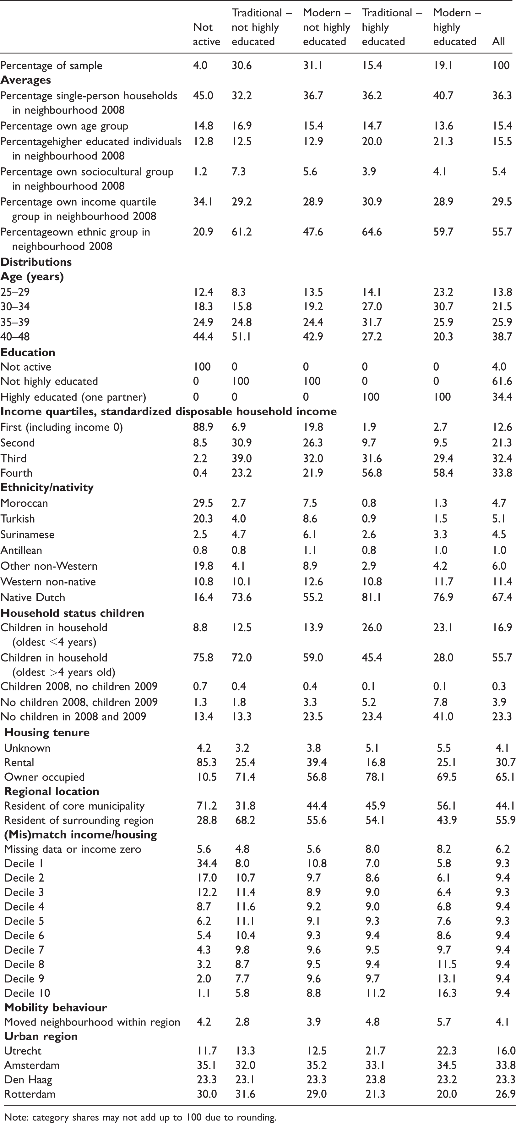
Note: category shares may not add up to 100 due to rounding.
Not active couples have, on average, the lowest percentage of their own group in the neighbourhood, which is due to the small size of this group (4% of the sample). They are ethnically diverse: the largest group (29.5%) has a Moroccan background. As expected, they are the poorest group, mostly living in rented dwellings (85.3%) that are relatively expensive compared to their income (34.4% in the lowest decile). For tenants, this discrepancy is likely compensated by rent regulation in social housing and by housing subsidies. Traditional not highly educated couples are the oldest group, and they are the least mobile within the urban region (2.8% moved), which is likely related to age and the high share of owner occupancy. Modern not highly educated couples are poorer and ethnically more diverse than the other economically active groups. The relatively low income of these couples indicates that female labour market participation might also be an economic necessity. Traditional highly educated couples often have young children (26.0%) or became parents during the observation period (5.2%). This group contained the highest share of homeowners (78.1%). Modern highly educated couples are the youngest group, and they have the highest incomes. They more often lived in dwellings that are relatively inexpensive compared to their incomes (16.3% in decile 10). They are more often childless (41.0%) but also more likely than other groups to have become parents between 2008 and 2009 (7.8%). They are the most mobile group within the urban region (5.7%).
Table 1 also reveals that sociocultural groups have specific geographies. Not active and modern highly educated couples are comparatively urban-oriented, while traditional not highly educated couples mostly live in suburban municipalities (68.2%). Additionally, we see differences across the four regions. There is an overrepresentation of both higher educated groups in the Utrecht region and an underrepresentation in the Rotterdam region. Not active and lower educated couples are overrepresented in the Rotterdam and Amsterdam regions (see Supplemental Material for more fine-grained geographies).
In sum, we see distinct sociocultural characteristics geographies, yet concentrations may overlap, Below, further analyses will establish whether sociocultural orientation is a salient dimension.
Multivariate regression
Model 1 (Table 2) shows the effect of the control variables on the probability of moving without any of the ‘neighbourhood match’ variables of interest. The model reveals that highly educated couples are more likely to move than not highly educated couples. Couples with children are more likely to move than couples without children. Moroccan, Turkish and other non-Western couples are less likely to make such moves. Couples outside the core municipalities (in the more suburban areas) move less often than couples in the core urban municipalities. Couples that live in relatively inexpensive dwellings (compared to their income) move more often, whereas couples that live in relatively expensive dwellings move less often. As expected, homeowners move less often than others. Couples living in neighbourhoods with a high share of single households move neighbourhoods more often, and contrary to expectations, couples living in neighbourhoods with a high share of similarly aged neighbours move more often as well.
Logistic regression multilevel models.
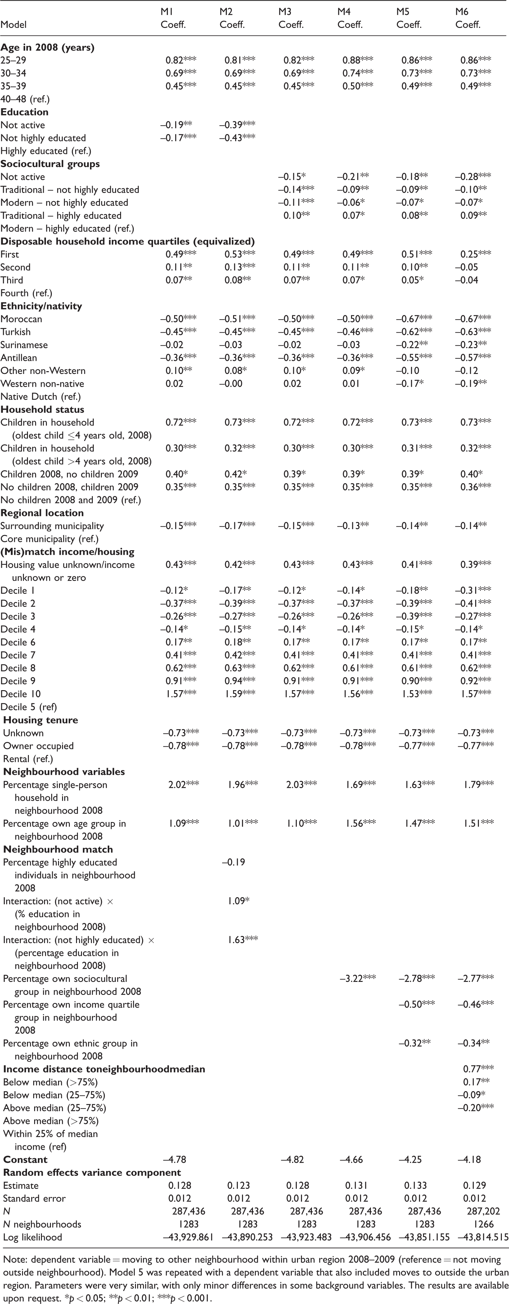
Note: dependent variable = moving to other neighbourhood within urban region 2008–2009 (reference = not moving outside neighbourhood). Model 5 was repeated with a dependent variable that also included moves to outside the urban region. Parameters were very similar, with only minor differences in some background variables. The results are available upon request. *p < 0.05; **p < 0.01; ***p < 0.001.
Model 2 introduces an interaction between education categories and share of highly educated at the neighbourhood level. The differences at the household level remain significant but the model also reveals an interaction with neighbourhood characteristics. For ease of interpretation, Figure 1 presents estimated probabilities (if p < 0.001) for these two variables in model 2. 10 The probability of not highly educated and not active couples moving out of the neighbourhood increases substantially as their neighbours are less similar. As the share of highly educated around them increases, the probability more than triples for not highly educated couples (from 3.3% to 10.4%). Highly educated couples see the reverse trend, yet less dramatically so. They are less likely to move as their neighbours are similarly educated.
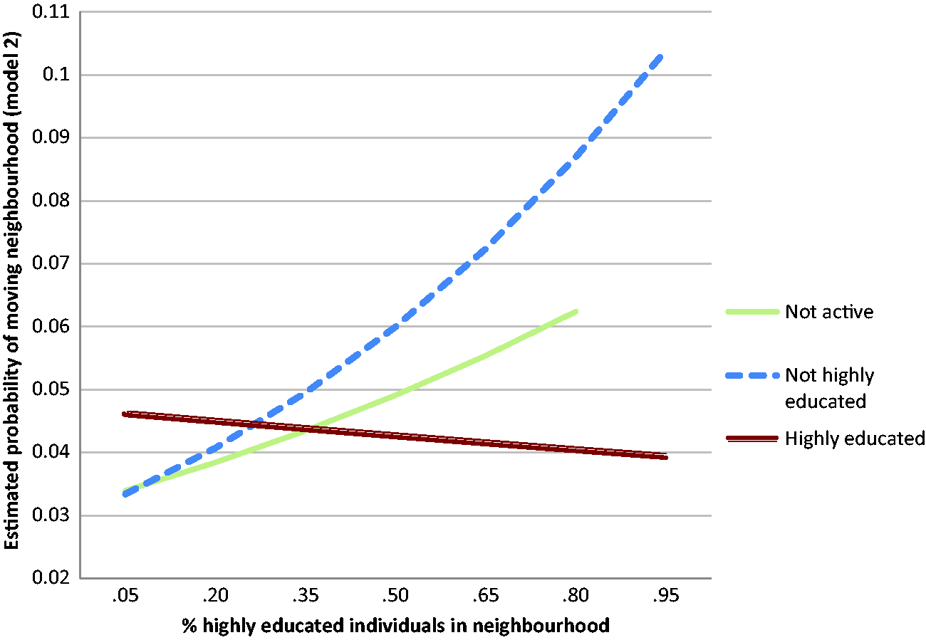
Predicted margins for education and percentage of highly educated individuals in the neighbourhood, 2008 (model 2).
The interaction effect gives us a clear image of how ‘neighbourhood match’ may impact mobility behaviour. Yet, this analysis is only possible with a binary variable, whereby a high share of one group implies a low share of the other. As mentioned, we are looking to refine our sociocultural analysis by introducing balance in income from work. This allows us to differentiate within education groups, and to estimate the sociocultural and the economic dimension separately in further models.
Model 3 shows estimates for the sociocultural categorization without any matching variables. The model indicates that these sociocultural groups show differences in mobility behaviour. Traditional highly educated couples are more likely to move than modern highly educated couples. All other groups are less likely to move.
Model 4 introduces the sociocultural match variable. As hypothesized, couples move less often when they live in neighbourhoods with high shares of other couples of the same sociocultural group. Model 5 adds the two other neighbourhood match variables: income match and ethnicity match. 11 These have similar effects: higher shares of the own group in the neighbourhood are associated with lower probabilities of moving. The effect of similar sociocultural composition decreases somewhat but remains strong and seems to be the most important determinant for couples.
To compare the effects of the three match variables, Figure 2 charts the estimated probabilities for model 5. All match variables have a negative effect on changing neighbourhood within the region. The slopes indicate that sociocultural match is estimated to have the largest negative effect. The steep slope is also the result of the comparatively low neighbourhood shares of our specific categorization. Also for this reason, we cannot estimate significant (p < 0.001) margins beyond 50% of own sociocultural group. Nevertheless, models with normalized and standardized match variables confirm that sociocultural match has the strongest impact on moving probability (additional models not shown).
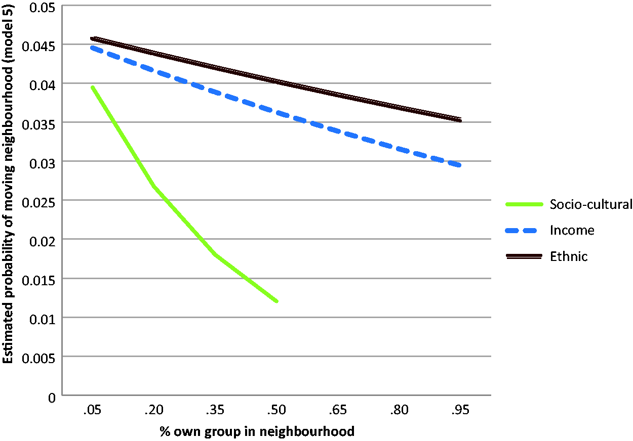
Predicted margins for percentage of own group in the neighbourhood, 2008 (model 5).
In model 6 we add the distance-to-median income variable as used by Musterd et al. (2016). This offers the opportunity to see how the distance variable ‘performs’ when controlling for the presence of own-group categories in the neighbourhood. It turns out that this and other matching coefficients all remain significant (p < 0.05). Adding the distance variable shows that the three ‘share of own group’ variables maintain their parameter values, while the distance variable adds somewhat to the model’s strength. Notably, while in the Musterd et al. (2016) paper (uncontrolled for own-group impact) the impact of the distance categories was U-shaped – larger distances from the median on both ends of the distribution added to the probability to move – the effect is now more linear. After controlling for the impact of the share of own group in the neighbourhood, for sociocultural, income and ethnic dimensions, having an income below the neighbourhood median still predicts moving away, yet having an above-median income is now a predictor for staying. This result may be explained by the inclusion of the own-group variables. For couples to have an above-median income is not a reason to leave when we take into account the presence of similarly disposed households. This model thus adds depth to our understanding of the effect of co-presence of ‘own group’ others, and of the distance between one’s income and the neighbourhood median on the probability to move (see also Galster and Magnusson Turner, 2017).
Key findings
Our models estimated the probability of couples moving neighbourhood within the urban region, controlling for individual-level attributes known for their potential impact, as well as for several ‘neighbourhood match’ variables. These variables represent the gap between the household’s own sociocultural disposition – operationalized in two ways – its own income status and one’s own ethnic or immigrant background, and the share of people in the neighbourhood with a similar sociocultural disposition, status or background. Accounting for household background and housing characteristics, we found that couples moved less often when they lived in neighbourhoods with high shares of other couples of the same education level and sociocultural group; the same was true for the two other neighbourhood match variables: income match and ethnicity match. The higher the share of own group in the neighbourhood, the lower the probability of moving. Predicted margins demonstrate that the sociocultural match has the largest effect. Living in a neighbourhood with a very low share of own-group sociocultural households would yield an estimated probability of moving that is substantially higher compared to living in a neighbourhood with a very high share of own-group sociocultural households. The absolute differences in moving probability may seem minor, but even mild preferences or small structural tendencies towards social homogeneity are potentially strong determinants for spatial segregation (Clark and Fossett, 2008; Schelling, 1971).
The outcome of segregation does require, however, that households move towards places where they find more similar neighbours. Paired t tests of the moves of sociocultural groups indicate that after moving, couples generally arrive in destination neighbourhoods with higher shares of own-group sociocultural households and in neighbourhoods with higher shares of own-group ethnic households (see the analyses in the Supplemental Material). Table 3 also shows that households tend to move to neighbourhoods with higher regional representations of their own group. In view of the low average shares of our sociocultural categories in neighbourhoods, we should note that these couples are likely not only drawn to our quite specific categorization. The found homogeneity and matching tendencies should be viewed as indicative of sorting among sociocultural groups that also include single-person households, ‘unstable’ and same-sex couples, and those outside our age categories. While not wholly separated, each group investigated has a specific and distinctive geography (see the Supplemental Material), thus confirming the literature on the fractious nature of class spatiality.
Shares of moving couples of departure neighbourhoods by destination neighbourhood.
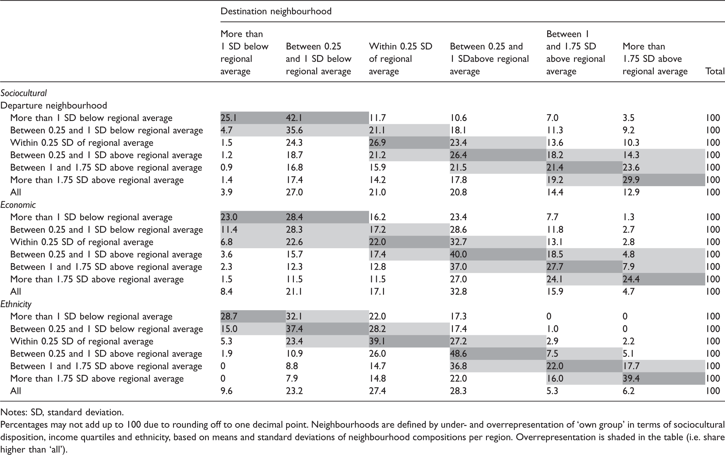
Notes: SD, standard deviation.
Percentages may not add up to 100 due to rounding off to one decimal point. Neighbourhoods are defined by under- and overrepresentation of ‘own group’ in terms of sociocultural disposition, income quartiles and ethnicity, based on means and standard deviations of neighbourhood compositions per region. Overrepresentation is shaded in the table (i.e. share higher than ‘all’).
Conclusions
We believe that our findings open new directions for research, as they confirm that economically active couples show a tendency towards homogeneity in their residential behaviour on three key dimensions. Each of the three dimensions has a significant effect on the probability of moving neighbourhood. When moving neighbourhood, couples tend to adapt by resettling in locations that contribute to closing the gap between themselves and their neighbours. Moreover, there is compelling evidence for our population that sociocultural fractures within and between classes not only play out spatially but even outweigh income or ethnic background as an explanation for residential mobility and spatial sorting. Of course, spatial class theory holds that these three dimensions are interdependent and mutually constitutive. Furthermore, our descriptive data and supplemental analyses indicate that, while dispositions produce distinctive patterns, sociocultural groups also overlap and may live in the same neighbourhoods (cf. Hanquinet et al., 2012).
The tendencies towards social homogeneity in residential sorting have implications for understanding urban stratification. While realizing that future studies would need to look at arrival neighbourhoods more closely, also in view of locally different housing market dynamics, our findings suggest that there are strong tendencies towards homogeneous neighbourhoods. This is similar to saying that, ceteris paribus, social homophily may produce segregation (Clark and Fossett, 2008; Schelling, 1971). This could have implications for urban development, especially in contexts in which policy efforts aim to reduce segregation. These aims are often translated into social mix policies. It should be recognized that social mixing at the neighbourhood scale goes against the homogeneity tendencies, as shown in this paper.
Given these implications, we would like to suggest three directions for further enquiry. First, our study sought to model sociocultural distinctions as understood in Bourdieu’s sociology and in gender-sensitive accounts of urban change. Our use of register data meant that we had to use relatively crude measures compared to purpose-built surveys and qualitative research, which can better gauge taste and consumption. It also meant that we had to limit ourselves to couples and to values on gender and work. These measures were revealing but sociocultural practices in employment are also structured by economic circumstances and institutional arrangements. 12 Future analyses may be able to use different strategies to analyse cultural and economic capital even more separately. For instance, the inclusion of data on the subject of study one is involved in or on the type of work one is engaged in may be revealing.
Second, our design and data availability limited our temporal scope. Also, our analysis focused on moderate-mobility crisis years. As people have fewer opportunities to move, particularly out of preference, sorting and segregation may diminish (Bailey, 2012). We expect that this has underestimated the effect of our matching variables. By making use of data over multiple years, new research would be better able to account for unobserved individual characteristics – possibly related to mutually constitutive characteristics of class and life course – in neighbourhood selection (see Galster and Magnusson Turner, 2017).
Third, our study was unable to investigate the impact of the spatial scale at which the processes towards homogeneity become manifest. Therefore, we could not answer questions such as: are individual households already satisfied with small-scale homogeneous areas? Or, is there a preference for larger homogeneous areas? Although there are neighbourhood effects studies that reveal the importance of the ‘block level’ (Andersson and Musterd, 2010; Johnston et al., 2004), such research did not focus on residential mobility. It is still largely unclear how the matching mechanisms operate for different social groups and for different types of neighbourhoods.
The question of scale is, nonetheless, highly relevant for urban planning and for the provision of local services. Given the persistence of anti-segregation and social mixing policies in the Western European context, a tendency towards social homogeneity may be problematic. Yet, if homogeneity at a small scale would suffice, urban development plans may still be able to ensure a level of social mix at larger scales. Homogeneous small neighbourhoods may, in the scenario just mentioned, be combined into heterogeneous larger neighbourhoods wherein people would still have the opportunity to meet frequently and to interact, such as when using public and commercial services or when bringing children to school. This ‘checker board model’ of urbanization would suit agendas that prioritize diversity and integration, while the smallest-scale neighbourhoods could be accepted as small and homogeneous places to live among households with approximately similar characteristics.
Supplemental Material
Supplemental material for Sociocultural, economic and ethnic homogeneity in residential mobility and spatial sorting among couples
Supplemental Material for Sociocultural, economic and ethnic homogeneity in residential mobility and spatial sorting among couples by Wouter van Gent, Marjolijn Das and Sako Musterd in Environment and Planning A: Economy and Space
Footnotes
Authors note
Marjolijn Das is also associated with the department of Geography, Planning and International Development Studies, Universiteit van Amsterdam, Amsterdam.
Acknowledgements
We would like to thank Jan Latten for his input during the conception of this study. Also, many thanks to Gelske van Daalen, Cody Hochstenbach, Fenne Pinkster, Bart Sleutjes and Aslan Zorlu, and the anonymous referees for providing comments on earlier versions of this paper. This paper presents results based on calculations by the authors using non-public microdata from the System of Social Statistical Datasets of Statistics Netherlands.
Declaration of conflicting interests
The author(s) declared no potential conflicts of interest with respect to the research, authorship and/or publication of this article.
Funding
The author(s) received no financial support for the research, authorship and/or publication of this article.
Notes
References
Supplementary Material
Please find the following supplemental material available below.
For Open Access articles published under a Creative Commons License, all supplemental material carries the same license as the article it is associated with.
For non-Open Access articles published, all supplemental material carries a non-exclusive license, and permission requests for re-use of supplemental material or any part of supplemental material shall be sent directly to the copyright owner as specified in the copyright notice associated with the article.